Abstract
Since the unsupervised segmentation of high-resolution remote sensing is a highly challenging task, the introduction of deep learning and processing may be a sensible choice to improve the quality of unsupervised segmentation. Unfortunately, any attempt to direct using unsupervised deep neural networks (UDNNs) to perform this task will be hindered by many obstacles: uncontrollable refinement processes, excessive fragmentation at the borders and excessive computing resource requirements. These obstacles can prevent us from obtaining acceptable results. To address this problem, this article proposes a hierarchical object-focused and grid-based deep unsupervised segmentation method for high-resolution remote sensing images (HOFG). Based on a grid approach, HOFG first adopt a lazy deep segmentation method (LDSM) to handle fragmentation and large image sizes. Then, a hierarchical and iterative segmentation strategy is introduced to reduce the accuracy expectation for the LDSM by means of a cascaded focus mechanism, making the entire segmentation process more controllable. HOFG can overcome all of the above obstacles while utilizing the high recognition ability of UDNNs. In experiments, HOFG are compared with shallow and deep unsupervised segmentation methods. The results show that HOFG can obtain fewer segments while maintaining a high accuracy. HOFG transform the unsupervised classification ability of UDNNs into a controllable and stable segmentation ability, making HOFG valuable for practical applications. The results show that on average, HOFG need only 81.73% as many segments as traditional shallow methods to achieve a high overall accuracy, and HOFG can obtain a 7.2% higher accuracy than a UDNN even when using only approximately 18% as many segments. HOFG can effectively and controllably utilize the recognition ability of UDNNs to achieve better unsupervised segmentation results.
1. Introduction
High-resolution remote sensing images contain many diverse ground features and can provide detailed spatial information for many geographical applications [1]. The traditional pixel-based methods are usually low in accuracy and exhibit various problems when processing high-resolution remote sensing images [2]. In object-based image analysis (OBIA), images are processed on the basis of having meaningful objects in the images rather than individual pixels, which can greatly improve the results for high-resolution remote sensing images [3,4]. OBIA has shown a superior performance compared to pixel-based methods in many studies and has become an important approach for processing very-high-resolution remote sensing images [5,6,7].
Unsupervised image segmentation methods, which can partition remote sensing images into meaningful segments (geo-objects), are foundational procedures for OBIA [8,9]. Through the integration of point/pixel, edge, region and texture features, unsupervised segmentation methods can generate homogeneous segments as the minimal units of an image, thereby greatly facilitating the fusion of knowledge in remote sensing image processing and analysis [10,11]. However, with the continuously increasing resolution of remote sensing images, the collected image data increasingly tend to contain high interclass homogeneity and intraclass heterogeneity; this characteristic makes it difficult to recognize high-quality segments based on shallow features [12].
Currently, when shallow models encounter difficulties, the most common approach is to resort to deep models, and indeed, the deep-learning-based methods for the supervised classification and semantic segmentation of remote sensing images have achieved great successes [13]. Through deep neural networks, higher-level features can be extracted, significantly improving the recognition accuracy for ground objects in remote sensing images [14,15]. For an unsupervised classification, unsupervised deep neural network (UDNN) methods are also available [16,17]. Unfortunately, although UDNNs have a high recognition ability, when these models are directly used for unsupervised segmentation, many obstacles arise, including uncontrollable refinement processes, excessive fragmentation at the border and excessive computing resource requirements (Section 3 will discuss these obstacles in detail). Although the direct use of UDNNs enables a much better recognition of ground objects in remote sensing images than is possible with shallow methods, the problems induced by these obstacles cause the corresponding unsupervised segmentation results to lack practical value. As a result, although deep learning remote sensing methods have been developed for many years, many remote sensing applications that require OBIA still rely on shallow segmentation methods to obtain segments; consequently, research on unsupervised remote sensing image segmentation is lagging behind the state of the art in the field of image processing.
To introduce deep learning into unsupervised remote sensing segmentation in a manner suitable for a practical application, this article proposes a hierarchical object-focused and grid-based deep unsupervised segmentation method for high-resolution remote sensing images (HOFG). Different from the traditional approaches, HOFG do not directly convert the output of a deep neural network into segments but rather constructs a grid to indirectly convert the segments; with the help of this mechanism, the corresponding lazy deep segmentation method (LDSM) can greatly suppress the generation of the fragments and support the handling of large input images. At the same time, HOFG do not rely on a neural network to recognize all segments simultaneously but instead uses a gradual focusing process that hierarchically proceeds from whole large objects to the detailed boundaries of those objects, thereby reducing the precision expectation of the LDSM and making the entire segmentation process more controllable. In experiments, HOFG are compared with three shallow and one deep unsupervised segmentation methods. The results show that HOFG retain the recognition ability of UDNNs, allowing it to obtain fewer segments while maintaining a high accuracy, and therefore it outperforms other methods in terms of the segmentation quality. Our article offers the following contributions:
- (1).
- Aiming at a practical use, we analyze the obstacles encountered when attempting to use a UDNN to obtain unsupervised remote sensing image segmentation results.
- (2).
- A hierarchical object-focused and grid-based method is proposed to address these obstacles. Specifically, lazy and iterative processes are used to gradually achieve unsupervised segmentation targets, rather than pursuing a powerful UDNN that can obtain excellent results in a single shot.
- (3).
- The unsupervised classification ability of UDNNs is transformed into a controllable and stable segmentation ability, making UDNN models suitable for practical remote sensing applications.
- (4).
- The proposed method can serve as a new framework for solving the problem of deep unsupervised segmentation in remote sensing. The corresponding source code is shared in order to motivate and facilitate further research on deep unsupervised remote sensing image segmentation.
2. Related Work
Remote sensing images can perform unsupervised segmentation and semantic segmentation.
2.1. Unsupervised Segmentation
Unsupervised segmentation or superpixel segmentation can partition images into segments (clusters). Currently, many shallow-method-based unsupervised remote sensing segmentation methods have been proposed, the majority of which rely on pixel thresholds or edge- or region-based techniques [18,19,20]. The parameters of the unsupervised segmentation methods have a significant impact on the results, and these parameters can be obtained from the spatial statistics of the segments [21,22,23]. Local measures can be used to control appropriate splitting and merging processes to mitigate the problems of undersegmentation and oversegmentation [24,25]. Optimal scale selection, noise weighting and outlier removal techniques allow segmentation methods to yield more accurate and reliable results [26,27]. Moreover, through the hierarchical selection of the scale, shape and compactness parameters, multiresolution segmentation (MRS) methods can be realized [28], and several software tools, such as eCognition, have proven to be successful for segmenting high-resolution remote sensing images. Notably, the contents of remote sensing images tend to vary greatly, and a single method often exhibits bias for certain types of content, hence, hybrid methods may need to be introduced into the segmentation process [29]. By employing region merging methods based on local and global thresholds, complementary methods can be combined to obtain better geo-object segmentation results [30]. In the computer vision research field, the high object recognition capabilities of deep neural networks can improve the quality of unsupervised segmentation. By extracting high-level semantic concepts, object categories can be segmented from images without preprocessing [31]. By distilling unsupervised features into high-quality discrete semantic labels, semantic segmentation discrete semantic labels can be discovered from the images [32]. The methods resulting from these studies perform well for datasets containing background objects (e.g., COCO), however, they are not designed for datasets with very large images or images with no relationship among background objects, and therefore, a further improvement of their processing strategy is needed to enable their application in the field of remote sensing.
2.2. Semantic Segmentation
In recent years, semantic segmentation networks, such as fully convolutional networks (FCNs), SegNet and U-Net, have been widely used in the semantic segmentation of remote sensing images [33,34]. These deep models not only can achieve end-to-end fast processing but also have a significantly higher pixel-level classification accuracy than traditional shallow models, so they have been widely used in a variety of remote sensing applications [35,36,37]. Semantic segmentation is data driven and requires a large number of training datasets for training; for remote sensing applications, these datasets may be difficult or require a huge cost to obtain [38]. Therefore, it is also important to use fewer annotations for semantic segmentation. Through unsupervised learning signals that account for neighborhood structures in terms of both space and features, remote sensing images can be segmented by sparse scribbled annotations [39]. By using clustering, spatial consistency and contrastive learning, single-scene semantic segmentation can be achieved without using any annotation [40].
This article mainly focuses on unsupervised segmentation or superpixels. When processing low- or medium-resolution remote sensing images, unsupervised segmentation methods can easily partition objects with homogenous features, and the resulting segments are closely related to the real geo-objects [41]. However, as the resolution continues to increase, intraclass heterogeneity becomes increasingly obvious, and precisely separating each geo-object becomes difficult to accomplish. Therefore, the following requirements for the unsupervised segmentation of very-high-resolution remote sensing images are usually specified:
- (i)
- Accurate boundary information and few cross-boundary segments
For most mapping applications, it is necessary to obtain accurate boundaries; when a segment crosses the boundary between different ground objects, this will inevitably introduce errors into the boundary analysis results [42]. In the absence of training samples, the easiest way to decrease the number of cross-boundary segments is to perform excessive oversegmentation, in which as many small segments as possible are generated to represent ground objects [43].
- (ii)
- Reasonably sized segments containing spatial information
In many remote sensing applications based on OBIA, it is necessary to further obtain morphological, shape or texture information from segments, which requires that each segment be of a reasonable size [44,45]. A segment that is too small may contain only some similar band information, while the spatial information is lost; consequently, excessive oversegmentation does not necessarily offer a good segmentation quality [46]. Furthermore, since the segments are the basic processing units for OBIA, some typical applications use segments to reduce the overall number of calculations, thus, too many and too small segments will hinder this goal [47].
To meet the above two requirements, traditional methods require the introduction of low-level statistics concerning the borders or segments to control the balance between splitting and merging. Unfortunately, with an increasing resolution, such low-level statistics have difficulty describing the characteristics of the segments [48], thus making these two requirements incompatible with each other for the traditional methods.
As an alternative, deep learning technology can be used to extract high-level features from images; in particular, it is very helpful for integrating color, texture, shape and context information into an object’s features [49]. By introducing a deep model, it is possible to understand objects and boundaries more accurately, which is beneficial for controlling the unsupervised segmentation process. For example, a deep autoencoder can be used to perform an unsupervised classification for multispectral or hyperspectral remote sensing images to obtain higher-quality classification results [50]. Through the iterative backpropagation processes performed in deep neural networks, unsupervised results can be obtained, and higher object recognition results can be achieved [17].
Nevertheless, although existing deep neural networks exhibit good unsupervised classification capabilities, if the corresponding results are converted into segments, these segments will have difficulty meeting the two requirements mentioned above (as will be discussed in detail in Section 3). Therefore, to the best of our knowledge, there is no deep unsupervised remote sensing segmentation method that is suitable for a practical use in the field of remote sensing OBIA. In high-resolution remote sensing image processing applications that simultaneously require OBIA and deep learning, a shallow and highly controllable method is usually adopted for OBIA, and a trial-and-error approach is used to achieve oversegmentation to meet the two requirements mentioned above [51].
Deep learning techniques have proven to be very effective in many studies. If we can adapt these techniques to the requirements of remote sensing unsupervised segmentation while maintaining their high recognition ability, we will be able to develop more valuable methods to improve research on remote sensing.
3. Obstacles Hindering Deep Unsupervised Remote Sensing Image Segmentation
Deep neural networks perform excellently in a supervised classification, semantic segmentation and object detection for remote sensing images. UDNNs have also been developed in the field of computer vision, and it is reasonable to expect that these UDNNs can also be applied to remote sensing images and achieve good unsupervised segmentation results. However, to date, the applications and methods regarding deep unsupervised remote sensing image segmentation have unfortunately remained scarce.
The reason is not that unsupervised remote sensing image segmentation has no research value, but rather that there are serious obstacles that hinder deep neural networks’ performance in the unsupervised segmentation of remote sensing images. In this section, we present an example to illustrate these obstacles. For a remote sensing image Iexample whose size is 600 × 600, we use a typical deep segmentation model Mexample trained via an unsupervised optimized backpropagation training process [16,17]. Mexample classifies Iexample to obtain the unsupervised classification results (the labels are randomly assigned), and pixels that are adjacent and have the same classification label are further assigned to a unique segment label. The corresponding results are shown in Figure 1.
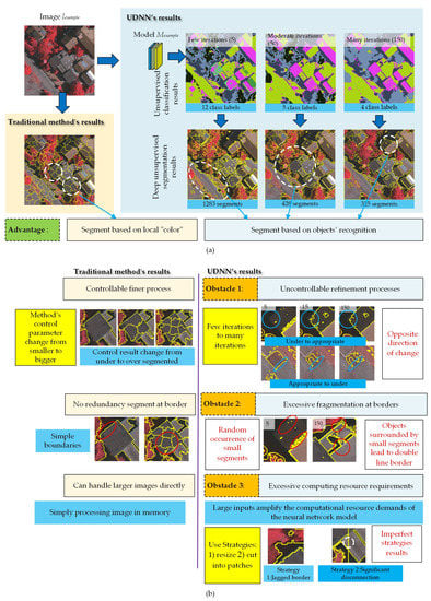
Figure 1.
Obstacles hindering deep unsupervised remote sensing image segmentation: (a) segmentation results of a UDNN; (b) illustrated obstacles.
In Figure 1a, we show deep results obtained with few iterations, moderate iterations and many iterations. Generally, as the number of iterations increases, the segments become larger, and the number of segments decreases. Compared with the results of the traditional shallow methods, the characteristics of deep methods are as follows:
Advantage: obvious superior recognition ability. It can be seen from Figure 1a that the deep model has an attractive advantage: in the deep segmentation results, buildings, roads and trees are separated into obvious and larger segments, reflecting the excellent ability of UDNNs to distinguish obvious ground objects. With either few or many iterations, the corresponding segments are very stably recognized.
UDNNs use high-level features instead of the specific local color space considered in traditional methods, so they perform better in the recognition of obvious objects. If this advantageous capability can be introduced into the unsupervised remote sensing image segmentation process, it will be very helpful for improving the segmentation quality and even achieving an object-by-object segmentation.
However, as shown in Figure 1b, UDNNs still face many obstacles in the unsupervised segmentation of remote sensing images.
(1) Obstacle 1: uncontrollable refinement process. Traditional methods can be used to easily control the iteration parameters, often shifting the segmentation result from undersegmentation to oversegmentation. This process can controllably obtain segmentation results from coarse to very fine.
UDNNs are difficult to control in this process: we selected two locations as examples. At location 1, in the results obtained with “few iterations”, part of the roof is not separated (undersegmentation); as the number of iterations increases, the roof is separated. At location 2, an area of grass is correctly separated in the results obtained with “few iterations”, but as the number of iterations increases, this location becomes undersegmented, and the boundaries of this area are destroyed.
The trends of these two locations conflict, and we cannot decide the direction of refinement by controlling the UDNN iterative process. We are unable to determine whether the segmentation results will be fine enough by modifying the iteration number, and large-scale cross-boundary segments will always exist randomly. Hence, no matter how the deep learning parameters and the number of iterations are adjusted, unacceptable segments will always exist in large regions, and because of the randomness of the training process, these erroneous regions may vary greatly each time the method is executed.
(2) Obstacle 2: excessive fragmentation at the border. For the results of the traditional methods, boundaries between their segments are made of simple borders, and this is a very common characteristic.
The UDNN results contain many very small fragments. For “few iterations”, which are random, very small segments exist at both the border and interior of larger ground objects, which lead to too many segments. For “more iterations”, these small segments are arranged on the boundary of the larger objects, forming a large number of rings and double-line boundaries.
Therefore, for UDNNs, no matter what we do, we will encounter a large number of random fragment segments, which will lead to the number of segments produced via deep learning to be much higher than that produced using the traditional methods. These small segments not only fail to effectively transmit spatial information but also have a negative impact on the subsequent analysis and calculations.
(3) Obstacle 3: excessive computing resource requirements. For the traditional methods, remote sensing images in certain conventional size ranges (e.g., smaller than 50,000 × 50,000) can be easily processed, thus, image “size” is an issue that does not require attention.
A UDNN model needs to be loaded into the GPUs memory for execution (processing a deep neural network using a CPU would be very slow). As the UDNNs input size increases, its overall demand for GPU memory increases exponentially. In particular, a computer equipped with 11 GB of video memory (our experimental computer) has difficulty loading a deep model that takes input images larger than 1000 × 1000, and remote sensing images are usually much larger than this size. For the segmentation of larger images, one of two strategies is usually adopted in the computer vision field. (i) Resizing to a smaller image: a large image is resized to a smaller image, the deep model processes the smaller image, and the results are then rescaled to the original size. This strategy of downscaling and subsequent upscaling leads to the boundary between two lower-resolution pixels becoming the boundary between the two objects of higher-resolution pixels, which may lead to a jagged boundary. (ii) Cutting into patches: since unsupervised labels are randomly assigned, the same label value is unlikely to correspond to the same object between two adjacent patches. Consequently, it is difficult to correctly overlap or fuse the separated patches to reintegrate the results, and this strategy can result in a significant disconnection at the borders of patches, thus creating false boundaries that do not exist in the original image.
Therefore, from the perspective of the application of value alone, deep unsupervised segmentation methods are very difficult to use for remote sensing images. Instead, traditional shallow methods are more controllable and practical. This is why, to date, there have been few applications of and little research on deep neural networks for an unsupervised remote sensing image segmentation.
However, it should also be recognized that as long as these three obstacles can be overcome, we can take advantage of the superior recognition capability of UDNNs to greatly improve the segmentation quality. Therefore, the main target of our research is to address these three obstacles to make UDNNs practically usable for an unsupervised remote sensing image segmentation.
4. Methodology
4.1. Overall Design of the Method
As analyzed in Section 3, UDNNs produce very attractive unsupervised segmentation results. Especially compared to shallow methods based on local color or texture features, deep neural networks can effectively recognize “objects” in complex high-resolution remote sensing data, and this characteristic is very important for the understanding and processing of remote sensing content.
However, we cannot practically use this capability of UDNNs unless we can overcome three obstacles: the uncontrollable segmentation process, uncontrollable fragmentation and the processing of large remote sensing images. Common attempts to do so usually rely on the proposal of a more complex and delicate deep neural network structure. Unfortunately, in the absence of training samples, it will be very difficult to design a “perfect” neural network with a sufficient subtle control of its iterations and parameters to effectively address these obstacles. Therefore, our approach does not rely on such an attempt to propose a complex and delicate deep neural network.
There are two strategies that have emerged in the fields of image processing and artificial intelligence (AI) that can help us solve the problem at hand:
- (1)
- Hierarchical: one may consider distinguishing the most obvious objects first, then further separating the most obvious region for each object and continuing this process until all boundary details can be distinguished. In this hierarchical iterative process, it is not necessary to recognize all segments in a single shot, it is only necessary to be able to subdivide the segments generated in the previous round.
- (2)
- Superpixel/grid-based: segment labels can be assigned to units based on superpixels or grid cells rather than single pixels. This can effectively prevent the formation of fragments that are too small, and the establishment of superpixel/grid boundaries can also suppress the emergence of jagged borders caused by the resizing process. At present, it is easy to obtain oversegmented results of uniform size using shallow unsupervised segmentation methods, and these results can be directly used as a set of superpixels or grid cells for this purpose.
Inspired by the above two strategies, this paper proposes a hierarchical object-focused and grid-based deep unsupervised segmentation method for high-resolution remote sensing images (HOFG). The overall design of HOFG is illustrated in Figure 2.
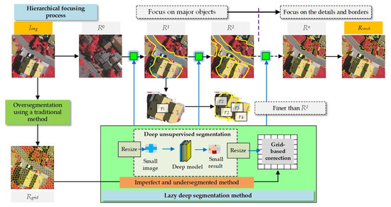
Figure 2.
Overall design of HOFG.
As shown in Figure 2, the input to HOFG is a remote sensing image Iimg, and the output is its corresponding segmentation results Rresult = {r1, r2, …, rn}, where ri = {seglabel, {pixel-locations}} is a segment defined in terms of the segment label seglabel and the corresponding pixel locations. In HOFG, a traditional shallow segmentation method is also used to perform an excessive oversegmentation to obtain the grid segment results Rgrid = {r1, r2, …, rn}. In Rgrid, it is necessary only to ensure the minimal occurrence of cross-boundary segments, and traditional methods can easily achieve this when the segments are sufficiently small and large in quantity. The segments in Rgrid are regarded as the smallest unit “grid cells” in HOFG, and all assignments of the segment labels in HOFG are based on these grid cells rather than on individual pixels.
A UDNN is adopted as the core of the deep segmentation model in HOFG, but it is not expected that all segments will be obtained by applying the UDNN only once, nor that the UDNN will exhibit a “perfect” performance. Instead, this paper proposes a lazy deep segmentation method (LDSM) for segment recognition, in which a relatively simple UDNN is used. The LDSM can process only input images that are smaller than a certain size and will recognize the most obvious objects in such an input image. In addition, the LDSM segmentation results are based on the grid cells in Rgrid, not individual pixels. These properties make the LDSM easier to realize than a “perfect” deep neural network.
On the basis of the LDSM, a hierarchical object-focused process is introduced in HOFG. First, the LDSM attempts to recognize the most obvious objects to obtain the first-round segmentation results R1, then, for each segment in R1, the LDSM performs another round of recognition and segmentation to obtain R2, which is finer than R1. Thus, the HOFG process is gradually refined from focusing on whole objects to focusing on the local details of the objects, and the final results Rsegment are obtained.
For HOFG, the initial segmentation result is R0 = {r1}, where r1 contains the entirety of Iimg. During subsequent iterations, the segment set Ri−1 obtained in the (i-1)th iteration is further separated into Ri in the ith iteration until the final segmentation results are obtained.
With the above design, we use deep neural networks in the LDSM and indirectly use the recognition ability of deep models; this enables the advantage discussed in Section 3 to be incorporated into the results. Moreover, the 3 obstacles discussed in Section 3 can be solved:
- (1)
- Uncontrollable refinement process: as the iterative process proceeds, Ri is refined on the basis of Ri−1, and the number of segments in Ri must be greater than or equal to the number in Ri−1. Therefore, although the number of segments identified by a UDNN is uncontrollable, the segmentation process of HOFG must be progressively refined as the number of iterations increases. This successfully solves Obstacle 1.
- (2)
- Excessive fragmentation at the border: due to the introduction of the grid-based strategy, the segment label of each grid cell is determined by the label of the majority of its internal pixels, and small pixel-level fragments do not appear in the results. Therefore, an excessive fragmentation at the border does not occur, overcoming Obstacle 2.
- (3)
- Excessive computing resource requirements: the use of downscaled input images in the LDSM can prevent UDNN from receiving excessively large images. This prevents the introduction of excessively large deep models during HOFG iterations, and the demand for GPU memory is always controlled within a reasonable range. Additionally, the segment boundaries in the output are directly based on the grid cells rather than the pixel-level UDNN results. Therefore, the use of downscaled input images in the UDNN (jagged boundary result) has little impact on the final results. These characteristics directly help address the challenges presented by Obstacle 3.
This process and the details of HOFG are described in Section 4.2 to Section 4.3.
4.2. Construction of the Grid and Initialization of the Set of Segmentation Results
For an input image Iimage, HOFG need to initialize two sets to support the execution of the whole method: (1) it needs to initialize the segmentation result set R0, which will serve as the input data for the first iteration of HOFG, and (2) it needs to construct the “grid” set Rgrid = {r1, r2, …, rn}, where the ri will be used as the basic units for segmentation.
For the initialization of the segmentation result set R0, because HOFG need to segment the entire image in the first iteration, R0 = {r1}; there is only one segment r1 in R0, and r1 contains all the pixels of the whole image.
To be suitable as the “grid” set for HOFG, Rgrid needs to satisfy two criteria: (1) regardless of what label is given, a segment that crosses a boundary will inevitably cause some pixels to be misclassified, destroying the corresponding boundary in the final results; therefore, there must be as few cross-boundary segments as possible in Rgrid. (2) Since the segmentation function in HOFG is performed by a neural network, an excessive segment height/width will detrimentally impact the layer-by-layer feature extraction, so the compactness of the segments needs to be high to ensure that the image surrounding each segment is close to a square.
To meet the above two criteria, HOFG adopt the simple linear iterative clustering (SLIC) algorithm, which is a traditional shallow unsupervised segmentation method. This algorithm is initiated with k clusters, Sslic = {c1, c2, …, ck}, with ci = {li, ai, bi, xi, yi}, where li, ai and bi are the color values of cluster ci in the CIELAB color space and xi and yi are the center coordinates of ci in the image. During the execution of the SLIC algorithm, there are two parameters that control the segmentation results. The first is the target number of segments, Pslicnum; the merging process will stop when the number of image segments is less than or equal to Pslicnum (the final number of segments is usually not strictly equal to Pslicnum). The second is the compactness parameter, Pcompact, which defines a balance between color and space, with a higher Pcompact giving more weight to the spatial proximity [52]. The ability to adjust Pslicnum and Pcompact makes the SLIC results more controllable. A larger Pslicnum can be specified to obtain oversegmented results and avoid the occurrence of cross-boundary segments, and a larger value of Pcompact can be specified to improve the compactness of each segment.
Based on the above discussion, the initialization process of HOFG is described in Algorithm 1.
| Algorithm 1: HOFG initialization algorithm (HOFG-Init) |
| Input: Iimg Output: Rgrid, R0 Begin Cinit-seg= Segment Iimg via SLIC with segments= Pslicnum and compactness= Pcompact; labelid=0; Rgrid=ø; R0=ø; foreach ci in Cinit-seg ri={labelid, {pixel positions of ci}}; Rgrid←ri; labelid= labelid+1; r1={0, {all pixel positions of Iimg}}; R0←r1; return Rgrid, R0; End |
Through the HOFG-Init algorithm, we obtain Rgrid and R0 for the HOFG method.
4.3. Lazy Deep Segmentation Method (LDSM)
As shown in Figure 2, HOFG do not try to obtain the segmentation result in just one step but transforms the segmentation process into an iterative process. In the initial stage, the segmentation result is R0, and R1 is obtained after the first iteration; after that, the i-th iteration converts Ri−1 to Ri. The LDSM acts as a bridge for each iteration, and the LDSM can be thought of as a mapping function that realizes Ri = LDSM(Ri−1).
4.3.1. Unsupervised Segmentation by a Deep Neural Network
HOFG employ a deep model Muc to perform an unsupervised pixelwise classification. Unsupervised deep models have a very different structure and training process than supervised models. For Muc, we adopt the strategy proposed by Kim and Kanezaki [16,17]. The model structure and the corresponding segmentation process are shown in Figure 3.
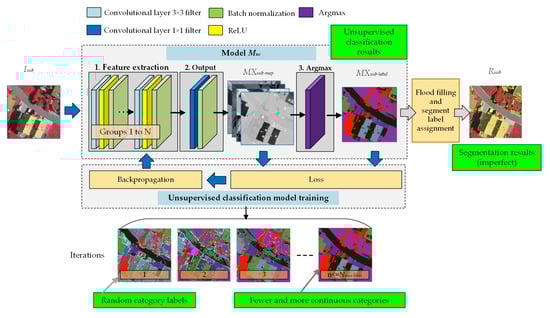
Figure 3.
Unsupervised deep neural network structure and segmentation process.
As shown in Figure 3, for the input subimage Isub, its size is Widthsub × Heightsub and the number of bands is Bandsub. Muc can perform an unsupervised classification of Isub and obtain results that assign a label to each pixel of Isub. For the unsupervised classification process of Muc, the maximum number of categories is Nmax-category, and the minimum number of categories is Nmin-category. There are three components in Muc:
- (1)
- Feature extraction component: this component contains N groups of layers, where each group consists of a convolutional layer (filter size is 3 × 3, padding is ‘same’ and the number of output channels is Nmax-category), a layer that applies the rectified linear unit (ReLU) activation function, and a batch normalization layer. Through this component, the high-level features of the input image can be extracted.
- (2)
- Output component: this component contains a convolutional layer (filter size is 1 × 1, padding is ‘same’ and the number of output channels is Nmax-category) and a batch normalization layer. Through the processing of these layers, a Widthsub × Heightsub × Nmax-category matrix MXsub-map is obtained, in which a number between 0 and 1 is used to express the degree to which each pixel belongs to each category.
- (3)
- Argmax component: this component uses the argmax function to process the matrix MXsub-map from the previous component to obtain Csub-label, which is a Widthsub × Heightsub × 1 matrix containing a discrete class label for each pixel.
Unlike in supervised neural networks, Muc needs to be initialized for each input Isub image. During the initialization, the weights of Muc are randomly assigned, so the output MXsub-label of an untrained Muc will be composed of random category labels in the range [0, Nmax-category-1]. At this point, there will be a difference between MXsub-map and MXsub-label; this difference can be used as the unsupervised loss function for the evaluation of the neural network:
Here, losscategory represents the loss of the output on the category labels, and it is expressed as follows:
where . Meanwhile, lossspace represents the constraint of spatial continuity, and it is defined as follows:
Thus, Formula (1) considers constraints on both feature similarity and spatial continuity [17]. Based on this loss, the weights of Muc can be adjusted through backpropagation, and this process can be iteratively repeated. As iteration progresses, MXsub-label will contain fewer categories (some categories will no longer appear in the results) that are more continuous (pixels with similar high-level features will be assigned to the same category). The corresponding training process is described in Algorithm 2.
| Algorithm 2: Unsupervised classification model training (UCM-Train) |
| Input:Isub, Nmax-train, Nmin-category, Nmax-category Output:Muc Begin Muc =Create model based on the size of Isub and Nmax-category; while (Nmax-train >0) [MXsub-map, MXsub-label]=Process Isub with Muc; loss= loss(MXsub-map, MXsub-label); Update weights in Muc←backpropagation with loss; Nmax-train= Nmax-train-1; Ncurrent-category=number of categories in MXsub-label; if (Nmin-category >= Ncurrent-category) break; return Muc; End |
For the UCM-Train algorithm, Nmax-category, Nmax-train and Nmin-category will all have an impact on the final results. For common unsupervised classification tasks, these parameters are difficult to specify, and doing so requires a large number of repeated tests. Fortunately, the LDSM is not required to produce perfect unsupervised classification results; it only needs to separate the most obvious objects in Isub.
Nmax-category determines the range of changes to the random class labels in the initial state; the larger the value specified for this parameter is, the more categories the model can recognize, but more iterations are also required to merge the pixels in each object. Nmin-category determines the fewest categories the model will recognize. The default values of these two parameters for HOFG are Nmax-category = 20 and Nmin-category = 3.
Nmax-train determines the maximum number of iterations; with a larger Nmax-train, Muc will output larger and more continuous classification segments, which is suitable for the classification of the overall image, while a smaller Nmax-train will make the classification more sensitive to category differences, suitable for the segmentation of boundaries and object details. For HOFG, the value of Nmax-train is related to the iteration sequence. By default, Nmax-train is 100 in the first iteration, 50 in the second iteration and 20 in the third iteration and later.
The results of Muc are unsupervised classification results, not segmentation results; pixels that are adjacent and have the same category label can be assigned the same segment label. Accordingly, the process of subimage segmentation by the deep neural network is described in Algorithm 3.
| Algorithm 3: Subimage segmentation by a deep neural network (SUB-Seg) |
| Input:Isub Output:Rsub Begin Muc =UCM-Train(Isub, Nmax-train, Nmin-category, Nmax-category); MXsub-label=Use Muc to process Isub; Rsub=ø; segid=1; seedpixel=first pixel in MXsub-label with label≠-1; while (seedpixel is not null) pixelpositions=Perform flood filling at seedpixel based on the same category label; MXsub-label[pixelpositions]=-1; Rsub ←{segid,{pixelpositions}} seedpixel=first pixel in Rsubi-classify with label≠-1; segid= segid+1; return Rsub End |
For a subimage Isub, the SUB-Seg algorithm first uses UCM-Train to train an unsupervised deep model Muc, which can generate the unsupervised classification results MXsub-label. SUB-Seg then uses the flood fill algorithm to find adjacent pixels with the same class label and assign them to the same segment; once all pixels have been assigned, SUB-Seg yields Rsub (the unsupervised segmentation results for Isub).
4.3.2. LDSM Process
The LDSM is responsible for segmenting each ri in Ri−1 to obtain a set of finer results, Ri. The LDSM uses the deep neural network model Muc and the SUB-Seg algorithm to perform the segmentation. The “lazy” nature of the LDSM is reflected in three aspects:
- (1)
- Low segmentation requirements: the LDSM focuses on the refinement of each segment obtained from the previous step of HOFG. Therefore, in the current step, SUB-Seg does not need to perform a perfect and thorough segmentation. Instead, for a separable ri, it is sufficient to find the most obvious different objects in it and separate it into >= 2 segments accordingly. This significantly reduces the difficulty of completing the SUB-Seg task.
- (2)
- Low segment border and pixel precision requirements: the basic segmentation units of the LDSM are the grid cells from Rgrid. Because a pixel-level fragmentation and the formation of jagged boundaries during the resizing are prevented by the grid-based strategy, the LDSM does not need to pursue precision at the level of all borders and pixels.
- (3)
- Low image size requirements: due to the relatively loose requirements of (1) and (2), when a large segment/image needs to be processed, the LDSM can directly downscale the image before processing it. This makes the LDSM easier to adapt to larger remote sensing images.
Based on the above characteristics, the process of the LDSM is shown in Figure 4.
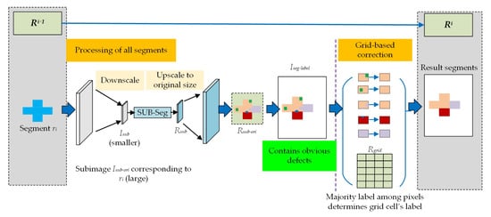
Figure 4.
Process of LDSM.
As shown in Figure 4, for an image Iimg and the corresponding segmentation results Ri−1, the LDSM can further separate Ri−1 to output finer segmentation results Ri. The LDSM can be divided into two stages:
- (1)
- Processing of all segments
For this step, the input is the segment set Ri−1 = {r1, r2, …, rn}, and the output is the segmented and labeled image Iseg-label. Each ri may need to be further separated into smaller segments. For ri, the corresponding rectangular image Isub-ori is cut from Iimg. Then, to focus on the segmentation task for ri, the pixels in Isub-ori that are not in ri are replaced with a constant background color.
We define a threshold value Pmax-size, which defines the maximum input image size for the LDSM. Isub-ori may be larger than the threshold size Pmax-size; in this case, it needs to be reduced to a size smaller than Pmax-size to obtain the input for SUB-Set, Isub. SUB-Seg will then process Isub to obtain the corresponding segmentation results Rsub; subsequently, Rsub will be resized to obtain the corresponding original-size results Rsub-ori. Based on the segments in Rsub-ori, pixel labels will be written into the image to obtain Iseg-label, which can be regarded as the refined segment image for Ri−1. Since the SUB-Seg algorithm itself is not perfect, fragments will be present in the results; at the same time, the process of downscaling and subsequent upscaling in the processing of each ri may produce jagged boundaries. Therefore, there will be many defects in Iseg-label, which will require a correction in the next stage.
- (2)
- Correction based on Rgrid
The grid cells in Rgrid are treated as the basic units of the segmentation process. The pixels within a grid cell must all be assigned the same segment label; to this end, the label of the majority of the pixels determines the label of the entire grid cell. In this way, unnecessary fragments that are too small can be filtered out, and the boundaries of the grid cells can be used to replace the jagged boundaries.
Based on the above stages, the corresponding process is described in Algorithm 4.
| Algorithm 4: Lazy deep segmentation method (LDSM) |
| Input:Iimg, Rgrid, Ri−1 Output:Ri Begin #Processing of all segments Iseg-label= Empty label image; globallabel=1; foreach ri in Ri−1 if (ri is too small) Iseg-label[pixel locations of ri]= globallabel++; continue; Isub-ori= Cut a subimage from Iimg based on a rectangle completely containing ri; Isub= Downscale Isub-ori if Isub-ori is larger than Pmax-size; Rsub= SUB-Seg(Isub); Rsub-ori= Upscale Rsub to the original size; foreach ri′ in Rsub-ori Iseg-label[pixel locations of ri′]= globallabel++; # Correction based on Rgrid Ri= ø; globallabel=1; foreach ri in Rgrid mlabel=Obtain the majority label among the pixels from Iseg-label[pixel locations of ri]; Iseg-label[pixel locations of ri]=mlabel; labellist=unique(Iseg-label); foreach li in labellist pixelpositions=find pixels in Iseg-label where label= li; Ri←{globallabel++,{pixelpositions}}; return Ri; End |
The LDSM can further separate the segments in Ri−1 to output Ri, where Ri is a finer segment set than Ri−1. By executing the LDSM multiple times, the segmentation results for Iimg can be gradually refined.
4.4. Hierarchical Object-Focused Segmentation Process
Based on the LDSM, HOFG iteratively and hierarchically narrow their focus from the entire remote sensing image to the details of the objects. This process is illustrated in Figure 5.
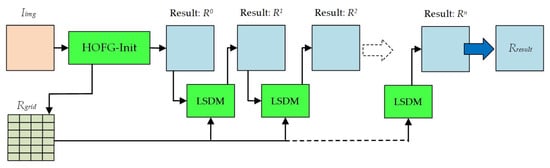
Figure 5.
Hierarchical object-focused segmentation process.
As shown in Figure 5, HOFG obtain R0 and Rgrid after initialization via the HOFG-Init algorithm. Starting from R0, the LDSM then continuously refines the segmentation results in sequence, producing R1, R2, … to Rn. The overall algorithm process is described in Algorithm 5.
| Algorithm 5: Hierarchical object-focused and grid-based deep unsupervised segmentation method for high-resolution remote sensing images (HOFG) |
| Input: Iimg, Nmax-iteration Begin:Rresult [R0, Rgrid]=HOFG-Init(Iimg); Ri−1=R0; inum=1; while (inum< Nmax-iteration) Ri=LDSM(Iimg, Ri−1, Rgrid); if (Ri has not changed compared to Ri−1) break; Ri−1=Ri; inum= inum+1; Rresult= Ri; return Rresult; End |
More iterations of HOFG will result in more segments. There are two termination conditions for HOFG: one is that the maximum number of iterations, Nmax-iteration, is reached, and the other is that Ri no longer changes from one iteration to the next. With the support of the LDSM, HOFG gradually separate Ri−1 into finer results Ri and gradually achieves the final segmentation goal.
5. Experiments
5.1. Method Implementation
In this study, all algorithms for HOFG were implemented in Python 3.7, the deep neural network was realized with PyTorch 1.7 and scikit-image 0.18 was used for image access/processing. All the methods were tested on a computer equipped with an Intel i9-9900K CPU with 64 GB of main memory and an NVIDIA GeForce RTX 2080Ti GPU with 11 GB of video memory.
To investigate the differences between HOFG and the traditional methods, we selected the following methods for a comparison:
- (1)
- SLIC: SLIC works in the CIELAB color space and can quickly gain momentum. SLIC is a relatively easy-to-control traditional shallow segmentation method, in which the target number of segments and the compactness of the segments can be specified [52].
- (2)
- Watershed: the watershed algorithm uses a gradient image as a landscape, which is then flooded from given markers. The markers parameter determines the initial number of markers, which, in turn, determines the final output results [53].
- (3)
- Felzenszwalb: the Felzenszwalb algorithm is a graph-based image segmentation method, in which the scale parameter influences the size of the segments in the results [54].
- (4)
- UDNN: a UDNN is used to classify a remote sensing image in an unsupervised manner [16,17], and segment labels are then assigned via the flood fill algorithm. As analyzed in Section 3, a UDNN cannot handle remote sensing images that are too large. Therefore, for large remote sensing images, we resize them to a smaller size that is suitable for processing on our computer and then restore the results to the original size before assigning the segment labels.
- (5)
- HOFG: for the method proposed in this article, the maximum input size Pmax-size of the LDSM is set to 600 × 600, and the maximum number of iterations, Nmax-iteration, is specified as five.
To test the segmentation capabilities of the five methods, we adopt the Vaihingen and Potsdam images from the ISPRS WG II/4 dataset. The characteristics of these images are summarized in Table 1.

Table 1.
Summary of the experimental image dataset.
5.2. Reference-Based Evaluation Strategy
A key criterion for the quality of unsupervised segmentation results is whether the segments destroy the boundaries of the ground objects. In this regard, a segment may exist in one of two situations: (i) the segment does not cross any object boundary, and all pixels in the segment are correct, or (ii) the segment crosses at least one boundary between two objects, and some pixels in the segment are incorrect. Based on this understanding, we use the strategy illustrated in Figure 6 to evaluate the accuracy of the segments.
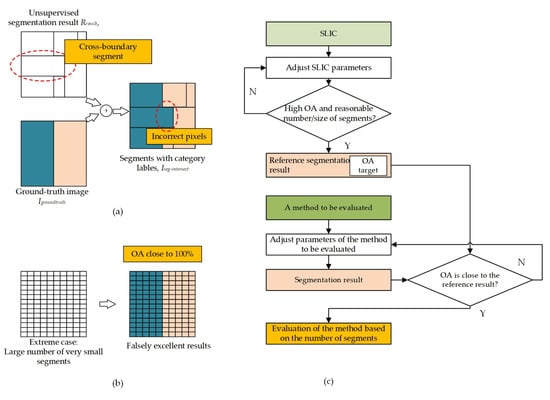
Figure 6.
Evaluation strategy: (a) obtaining the OA of a set of segmentation results; (b) extreme results in which the OA is very high but comparative value is lost; and (c) evaluation method based on a reference OA.
As shown in Figure 6a, to evaluate a set of unsupervised segmentation results Rresult, we can introduce a ground-truth image Igroundtruth. For each segment ri in Rresult, its intersection with Igroundtruth is taken, and the category label associated with the largest proportion of the pixels is regarded as that segment’s ground-truth category label; once all segments have been assigned a category label in this way, Iseg-intersect is obtained. We adopt the overall accuracy (OA) to describe the accuracy of Iseg-intersect:
where Npixels is the number of pixels in Igroundtruth and Ncorrect-pixels is the number of pixels with correct category labels in Iseg-intersect. We also adopt the mean intersection over union (mIoU) as the evaluation metric. For a certain category i, the intersection over union (IoU) is defined as follows:
where Rgt-i is the set of pixels belonging to category i in Igroundtruth and Rseg-i is the set of pixels belonging to category i in Iseg-intersect. The mean IoU (mIoU) is defined as follows:
Nevertheless, the OA metric CANNOT be used as the sole criterion for evaluating the results of an unsupervised segmentation algorithm. As shown in Figure 6b, for a set of segmentation results, when the number of segments is large and the size of the segments is sufficiently small, any segments that cross a boundary will also be very small. Under such extreme conditions, such as one pixel corresponding to one segment, the OA value can reach 100%. All the methods participating in a comparison may be capable of producing very small segments and consequently reaching OA values approaching 100%, but this does not necessarily mean that all the corresponding methods are excellent. Therefore, a good segmentation evaluation method needs to consider both the OA and the number of segments.
As shown in Figure 6c, our evaluation strategy is based on reference results. Since SLIC is a traditional segmentation method in which the number and compactness of the segments can be easily controlled, we select SLIC as the reference method. By adjusting the SLIC parameters, we can obtain a high OA score = x while ensuring that the segments are of a reasonable number and size. The corresponding SLIC results are then taken as the reference against which to measure the segmentation quality. Since the OA variations of the various methods are not linear, it is impossible to obtain an OA strictly equal to x; therefore, we consider a value close to or greater than x to reach the OA target. For methods (2)–(5), we adjust the parameters to attempt to achieve an OA in the interval of [x-0.5%, 100%] with as few segments as possible. The parameter settings for all methods are given in Table 2.
Table 2.
Parameter settings for all methods.
For similar OA scores, a method that can produce fewer and larger segments is considered to have a higher object recognition ability, indicating that this method is better; otherwise, its recognition ability and, thus, its segmentation quality are lower.
5.3. Iterative Process of HOFG and Comparison of Results
In this section, we again use the image patch in Figure 1 as the test image. First, method (1), the SLIC method, is used as the reference method. For this test image, target segments = 400 and compactness = 10 are used as the SLIC method’s parameters, and OA = 91.75% is obtained. With the goal of reaching or exceeding this accuracy, four iterations of HOFG are performed, with the results being shown in Figure 7.
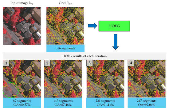
Figure 7.
The iterative process of HOFG.
As shown in Figure 7, SLIC with a segment number parameter of 600 is adopted in the HOFG to initialize Rgrid, which finally contains 516 segments, then, the iterative process of the HOFG begins. In the first iteration, only 82 segments are generated; from the whole image, the large areas of houses, roads and trees are segmented, yielding results close to the ideal target of “one object corresponding to one segment” for OBIA. From these results, it can be seen that as a deep method, HOFG have obvious advantages compared with traditional shallow methods, however, the results of the first iteration also have some defects. For example, in the region enclosed by the green circle, some large-scale ground objects are connected together (corresponding to a large cross-boundary segment). Consequently, the OA is only 80.57%, failing to surpass the OA of the reference SLIC results. As the iterative process continues, the second iteration produces 143 segments with OA = 87.48%, and the third iteration produces 221 segments with OA = 91.11%. Finally, in the fourth iteration, OA = 92.04%, and the number of segments is 247. At this time, the accuracy of HOFG exceeds the reference accuracy of SLIC, indicating that there is no need to perform further iterations.
For all five methods participating in the comparison, their segmentation results for this test image are shown in Figure 8.
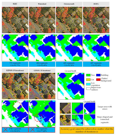
Figure 8.
Segmentation results of the five methods.
The corresponding OA values and numbers of segments are listed in Table 3.
Table 3.
OA and segment number comparison of the five methods.
As seen in Figure 8 and Table 3, with SLIC as the reference method, both the watershed and Felzenszwalb algorithms can achieve the OA target, but they need to generate more segments to achieve this accuracy. For the watershed algorithm, the number of segments is 484, and for the Felzenszwalb algorithm, the number of segments is 428. Among the three shallow methods, SLIC uses the fewest segments to achieve better results, which is why in many OBIA applications for remote sensing, SLIC is the preferred segmentation algorithm.
For the UDNN method, we consider the segmentation results obtained after both 5 iterations and 15 iterations; the reason for performing these two consecutive tests is to show that no matter what training parameters are assigned, it is very difficult for a UDNN to achieve the OA target. With five iterations, the UDNN generates many large-area cross-boundary segments, seriously affecting its accuracy, and the OA is only 84.81%. Moreover, this low number of iterations also results in a serious fragmentation, and the number of segments is the highest at 1346 (note that this number is different from the number of segments in Figure 1 because the neural network training process is subject to a certain level of randomness). With 15 iterations, not only are the problems seen after 5 iterations not solved, but new problems also emerge. As shown in Figure 7, stripe-shaped and connected segments appear at the boundaries of objects, thus introducing more errors into the segmentation results and causing the OA to decrease to 77.40%, while the number of segments is reduced to 773. Although obvious objects are recognized by the UDNN, the low OA and the excessively large number of segments causes the UDNN results to lack a practical remote sensing application value.
In contrast, HOFG obtain OA = 92.04% and number of segments = 247, achieving the highest accuracy with the fewest segments among all the methods. HOFG can obtain an OA that is 7.2% higher than that of the UDNN by using only approximately 18% as many segments. The above results also show that Obstacles 1 and 2, identified in Section 3, are overcome, indicating that HOFG has the following advantages:
Overcoming Obstacle 1: the segmentation refinement process is controllable. As shown in Figure 7, segmentation with HOFG is a process of a step-by-step refinement. In each iteration, HOFG split the large segments identified in the previous iteration into smaller segments. Accordingly, a reasonable OA goal can be achieved by controlling the number of iterations of the HOFG process.
Overcoming Obstacle 2: the fragmentation and stripe-shaped segments are suppressed. In HOFG, the segments are not directly generated from the unsupervised classification output of a UDNN, instead, Rgrid is used as a filter to suppress the fragmentation and stripe-shaped segments. This strategy guarantees that the number and size of the generated segments will be within a reasonable range.
Because of the above two characteristics, HOFG inherit the advantages of deep learning methods while avoiding their typical shortcomings, thereby endowing HOFG with a practical application value.
5.4. Performing Segmentation on Larger Remote Sensing Images
To test the performance of HOFG on larger remote sensing images, we adopt two remote sensing images from the ISPRS dataset: (1) test image 1, from the Vaihingen image file “top_mosaic_09cm_area11.tif”, with dimensions of 1893 × 2566, and (2) test image 2, from the Potsdam image file “top_potsdam_2_10_RGB.tif”, with dimensions of 6000 × 6000.
These two images are relatively large. The three shallow methods can easily process these images, however, a neural network model constructed based on such a large input size would be very large, far beyond what our computer’s GPU could load. Therefore, to segment these large images using a UDNN, the strategy is to downscale them to a smaller size to perform the segmentation and then upscale the segmentation results to the original size afterward. HOFG have their own mechanism for processing large images and therefore can directly process these two images.
The test images and their corresponding ground-truth segmentation images and segmentation quality evaluation results are shown in Figure 9a.
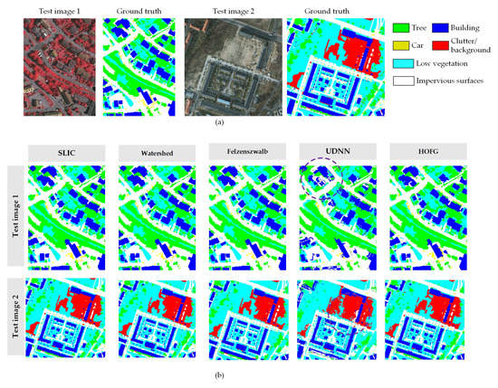
Figure 9.
Test images and segmentation quality evaluation results: (a) test images and ground truth; (b) segmentation results with category labels.
The segmentation results for the two images, along with their category labels, are presented in Figure 9b. Since the images are very large and the numbers of segments are similarly large, it is difficult to clearly see any individual segments once the images have been sized for presentation in this paper, so Figure 9b does not list the segmentation results of the methods. We show the examples of detailed differences in the local areas in Figure 10.
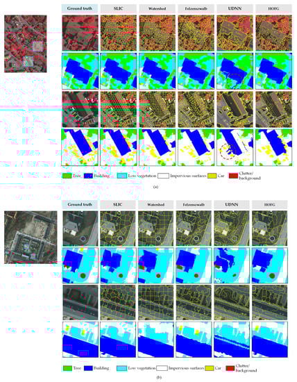
Figure 10.
Detailed comparisons of the five methods on test images 1 and 2: (a) segmentation results for test image 1; (b) segmentation results for test image 2.
Due to the high OA target, the labeled segmentation results of all the methods except for the UDNN method are fairly similar. The UDNN cannot reach the reference OA, and fragmentation can also be seen in Figure 9 (marked with circles). Taking the SLIC method as the reference method, the performance of the five methods is shown in Table 4.
Table 4.
Quality evaluation on two test images.
For test image 1, the initial segment number parameter of SLIC is specified as 7000, and the number of segments obtained after an algorithm execution is 5799. For test image 2, the initial segment number parameter of SLIC is specified as 9000, and the final number of segments obtained after the algorithm execution is 7882. With SLIC as the reference method, the watershed algorithm needs more segments to achieve a corresponding OA, whereas the number of segments produced by the Felzenszwalb algorithm is close to that of SLIC. For the UDNN method, as discussed in Section 5.3, it is impossible to achieve the target OA, so we choose a set of output results with a reasonable number of segments and a relatively high OA. It can be seen that the number of segments generated by the UDNN is much higher than the number produced by the shallow methods, which again proves that a UDNN is not suitable for directly performing an unsupervised segmentation of the remote sensing images. In contrast, HOFG achieve the OA goal with the fewest segments among all the methods. Detailed comparisons of the five methods on test image 1 are shown in Figure 10.
As seen from Figure 10a,b, the three shallow unsupervised segmentation methods (SLIC, watershed and Felzenszwalb) cannot truly distinguish objects in remote sensing images; their segmentation results are based only on local color clustering, thresholding or graph results. Due to this focus on local characteristics, a larger image size affects only the processing time, so these shallow methods can be effectively adapted to the processing of large remote sensing images.
For the UDNN, some attractive results can be observed in Figure 10a: buildings, trees and impervious surfaces are all identified as large, whole segments. Unfortunately, however, it can also be observed that some segments span multiple objects (marked with red circles), and due to the image downscaling and upscaling process, the segment boundaries exhibit a certain sawtooth phenomenon. These problems directly decrease the segmentation accuracy of the UDNN. In Figure 10b, since test image 2 is much larger, the UDNN needs to perform a downscaling and upscaling to an even greater extent, so the sawtooth phenomenon is more obvious, and some building boundaries are even destroyed. As seen from these results, a UDNN has the high recognition ability characteristic of deep neural networks, but many uncontrollable problems directly affect the final results. Especially for large remote sensing images, the problems of sawtooth boundaries, cross-boundary segments and broken boundaries become more obvious.
Regarding the results of HOFG, it can be seen that on the one hand, HOFG can use larger segments to capture objects in an image, and buildings, roads and cars are all recognized, indicating that HOFG retain the recognition ability of deep neural networks. On the other hand, for both test image 1 and test image 2, the large size of these images does not lead to undesirable results of HOFG, and segments with relatively accurate boundaries can still be obtained. From the results in Figure 10a,b, it can be inferred that HOFG can be successfully used for the processing of large remote sensing images to achieve a higher-quality segment recognition. Specifically, HOFG have the following advantage:
Overcoming Obstacle 3:
For test images 1 and 2, the 11 GB of GPU memory provided in this experiment is insufficient to directly load the corresponding UDNN models. HOFG provide a mechanism to reduce the computational resource requirements and thus have the ability to process large remote sensing images. Due to the use of the grid strategy and the LDSM, HOFG can handle large remote sensing images and obtain reasonable boundaries and segments.
Processing large remote sensing images is a necessary ability of any practically applicable method in this field, and HOFG have this ability, allowing it to play a role in practical applications.
5.5. Execution Time Comparison
To analyze the execution times of the methods, we use the five methods to process the test images and run each method five times. The average execution time comparison of the five methods is shown in Table 5.
Table 5.
Execution times of different algorithms on the remote sensing test images.
The execution times of the three shallow methods, SLIC, Watershed and Felzenszwalb, are directly associated with the number of pixels; the larger the number of pixels is, the longer the time. There is no obvious difference in the speeds of these three methods. The UDNN uses a size reduction strategy; in this example, the size of test image 2 is 6000 × 6000, while the UDNN uses only a 600 × 600 input, which is equivalent to reducing the amount of data and the number of computations by 10 × 10 = 100 times. Thus, the UDNN is the fastest among all the methods for test image 2. HOFG need to use SLIC to obtain Rgrid and then perform multiple rounds of UDNN processing on many subimages. Although the quantity of input data for each processing step is small, the run time of the method increases. Among all the methods, HOFG are the slowest, especially for test image 2, and HOFG need close to 15 min to run. Although this time is barely acceptable, the speed of HOFG could be increased. From the experimental results, we note that the UCM-Train algorithm of HOFG needs to run completely from the initial state in each iteration process, which will consume a considerable execution time of the HOFG. In future work, we will start to improve UCM-TRAIN so that it can continue the experience of the previous iteration of HOFG, which will greatly improve the training speed of HOFG.
5.6. Experiments on More Remote Sensing Images
To test the remote sensing processing capabilities of HOFG more extensively, this section introduces more remote sensing image files, the details of which are listed in Table 6.
Table 6.
Details of additional remote sensing test images.
As shown in Table 6, we consider 10 high-resolution remote sensing images, of which images 1 to 5 are from the Vaihingen dataset and images 6 to 10 are from the Potsdam dataset. For the reference SLIC method, segmentation number = 7000 is used for all Vthe aihingen images, and segmentation number = 9000 is used for all the Potsdam images. The Rgrid parameter of the HOFG is Pslicnum = (1.5 × SLIC parameter), and the HOFG process is iterated to achieve the same OA as that of the reference SLIC results. The results for the ten images are compared in Table 7.
Table 7.
Comparison of SLIC and HOFG results on 10 images.
As shown in Table 7 and analyzed in the previous sections, HOFG are a controllable segmentation method and can therefore reach the target OA for all the images. Regarding the number of iterations needed to reach the OA target, most images require four iterations; the exception is image 7, which requires five iterations. For all images, HOFG produce fewer segments than SLIC. The “Percentage” column of Table 6 presents the value of (the HOFG segment number)/(SLIC segment number) × 100%; from this column, it can be seen that for these remote sensing images, HOFG can achieve an OA similar to that of SLIC, with 81.73% as many segments as SLIC on average. Among the test images, HOFG perform the best on image 5, needing only 69.39% as many segments as SLIC to achieve a comparable segmentation accuracy.
6. Conclusions
To better analyze complex high-resolution remote sensing data via segmentation, we need to take advantage of the higher object recognition ability offered by deep learning to improve the results of the unsupervised segmentation methods. However, directly converting the output of a UDNN into segments does not result in an improved segmentation effect; indeed, in most cases, the results of a UDNN are inferior to those of shallow methods.
This paper proposes a hierarchical object-focused and grid-based deep unsupervised segmentation method for high-resolution remote sensing images (HOFG). By means of an iterative and incremental improvement mechanism, HOFG can overcome the problems caused by the direct use of UDNNs and yield superior unsupervised segmentation results. Experiments show that HOFG have the following advantages.
- (1)
- Inheriting the recognition ability of deep models: in place of shallow models, a UDNN is adopted in HOFG to identify and segment objects based on the high-level features of remote sensing images, enabling the generation of larger and more complete segments to represent typical objects such as buildings, roads and trees.
- (2)
- Enabling a controllable refinement process: with the direct use of a UDNN, it is difficult to control the oversegmentation or undersegmentation of the results; consequently, a UDNN is unable to achieve a given OA target. In HOFG, the LDSM is used in each iteration to refine the results from the previous iteration; this ensures that the segments can be progressively refined as the iterative process proceeds, thus making the HOFG segmentation process controllable.
- (3)
- Reducing fragmentation at the border: a reference grid is used in the LDSM, and the UDNN results are indirectly transformed into segments on the basis of this grid. In this way, segments that are too small, stripe shaped or inappropriately connected can be filtered out.
- (4)
- Providing the ability to process large remote sensing images: as the input image size increases, the corresponding UDNN model will also increase in size, making it difficult for ordinary GPUs to load. Consequently, the direct use of a UDNN requires a resizing of the input image, which can lead to jagged segment boundaries. The grid-based strategy of the LDSM and the iterative improvement process in HOFG reduces the detrimental influence of resizing, allowing HOFG to obtain high-quality segmentation results even when processing very large images.
HOFG also have shortcomings: the speed of HOFG is slower than the traditional shallow model methods. The key factor affecting the execution speed lies in the UCM-TRAIN algorithm. By improving the training strategy of UCM-TRAIN, the execution time of HOFG can be significantly reduced. We will focus our research on this issue to make HOFG more useful in the field that needs to obtain results quickly or repeatedly.
HOFG not only inherit the advantages of deep models but also avoids the problems caused by the direct use of deep models; thus, it can obtain superior results compared to either shallow or other deep methods. Moreover, its controllability and relatively stable performance make HOFG as easy to use as the normal shallow unsupervised segmentation methods. HOFG thus combine the advantages of both shallow and deep models for unsupervised remote sensing image segmentation and provide a way to utilize deep models indirectly. As a result, it has a theoretical significance for exploring the applications of deep learning in the field of remote sensing.
Author Contributions
Conceptualization, X.P. and X.L.; data curation, J.Z.; methodology, X.P.; supervision, J.X.; visualization, J.Z.; writing—original draft, X.P. All authors have read and agreed to the published version of the manuscript.
Funding
This research was jointly supported by the Strategic Priority Research Program of the Chinese Academy of Sciences (Grant No. XDA28110502), the National Natural Science Foundation of China (41871236; 41971193), the Foundation of the Jilin Provincial Science & Technology Department (20200403174SF, 20200403187SF) and the Foundation of the Jilin Province Education Department (JJKH20210667KJ).
Data Availability Statement
Not applicable.
Conflicts of Interest
The authors declare no conflict of interest.
References
- Pan, X.; Zhao, J.; Xu, J. An object-based and heterogeneous segment filter convolutional neural network for high-resolution remote sensing image classification. Int. J. Remote Sens. 2019, 40, 5892–5916. [Google Scholar] [CrossRef]
- Castillejo-González, I.L.; López-Granados, F.; García-Ferrer, A.; Peña-Barragán, J.M.; Jurado-Expósito, M.; de la Orden, M.S.; González-Audicana, M. Object-and pixel-based analysis for mapping crops and their agro-environmental associated measures using QuickBird imagery. Comput. Electron. Agric. 2009, 68, 207–215. [Google Scholar] [CrossRef]
- Castilla, G.; Hay, G.G.; Ruiz-Gallardo, J.R. Size-constrained region merging (SCRM). Photogramm. Eng. Remote Sens. 2008, 74, 409–419. [Google Scholar] [CrossRef]
- Blaschke, T. Object based image analysis for remote sensing. ISPRS J. Photogramm. Remote Sens. 2010, 65, 2–16. [Google Scholar] [CrossRef]
- Blaschke, T.; Hay, G.J.; Kelly, M.; Lang, S.; Hofmann, P.; Addink, E.; Feitosa, R.Q.; van der Meer, F.; van der Werff, H.; van Coillie, F. Geographic object-based image analysis–towards a new paradigm. ISPRS J. Photogramm. Remote Sens. 2014, 87, 180–191. [Google Scholar] [CrossRef] [PubMed]
- Fu, B.; Wang, Y.; Campbell, A.; Li, Y.; Zhang, B.; Yin, S.; Xing, Z.; Jin, X. Comparison of object-based and pixel-based Random Forest algorithm for wetland vegetation mapping using high spatial resolution GF-1 and SAR data. Ecol. Indic. 2017, 73, 105–117. [Google Scholar] [CrossRef]
- Gong, M.; Zhan, T.; Zhang, P.; Miao, Q. Superpixel-based difference representation learning for change detection in multispectral remote sensing images. IEEE Trans. Geosci. Remote Sens. 2017, 55, 2658–2673. [Google Scholar] [CrossRef]
- Pekkarinen, A. A method for the segmentation of very high spatial resolution images of forested landscapes. Int. J. Remote Sens. 2002, 23, 2817–2836. [Google Scholar] [CrossRef]
- Wang, M.; Li, R. Segmentation of high spatial resolution remote sensing imagery based on hard-boundary constraint and two-stage merging. IEEE Trans. Geosci. Remote Sens. 2014, 52, 5712–5725. [Google Scholar] [CrossRef]
- Dey, V.; Zhang, Y.; Zhong, M. A Review on Image Segmentation Techniques with Remote Sensing Perspective. In Proceedings of the ISPRS TC VII Symposium–100 Years ISPRS, Vienna, Austria, 5–7 July 2010; Volume 38. [Google Scholar]
- Yi, L.; Zhang, G.; Wu, Z. A scale-synthesis method for high spatial resolution remote sensing image segmentation. IEEE Trans. Geosci. Remote Sens. 2012, 50, 4062–4070. [Google Scholar] [CrossRef]
- Wang, F.; Piao, S.; Xie, J. CSE-HRNet: A context and semantic enhanced high-resolution network for semantic segmentation of aerial imagery. IEEE Access 2020, 8, 182475–182489. [Google Scholar] [CrossRef]
- Ma, L.; Liu, Y.; Zhang, X.; Ye, Y.; Yin, G.; Johnson, B.A. Deep learning in remote sensing applications: A meta-analysis and review. ISPRS J. Photogramm. Remote Sens. 2019, 152, 166–177. [Google Scholar] [CrossRef]
- Zhang, C.; Yue, P.; Tapete, D.; Jiang, L.; Shangguan, B.; Huang, L.; Liu, G. A deeply supervised image fusion network for change detection in high resolution bi-temporal remote sensing images. ISPRS J. Photogramm. Remote Sens. 2020, 166, 183–200. [Google Scholar] [CrossRef]
- Zhang, L.; Hu, X.; Zhang, M.; Shu, Z.; Zhou, H. Object-level change detection with a dual correlation attention-guided detector. ISPRS J. Photogramm. Remote Sens. 2021, 177, 147–160. [Google Scholar] [CrossRef]
- Kanezaki, A. Unsupervised Image Segmentation by Backpropagation. In Proceedings of the 2018 IEEE International Conference on Acoustics, Speech and Signal Processing (ICASSP), Calgary, AB, Canada, 15–20 April 2018; pp. 1543–1547. [Google Scholar]
- Kim, W.; Kanezaki, A.; Tanaka, M. Unsupervised learning of image segmentation based on differentiable feature clustering. IEEE Trans. Image Process. 2020, 29, 8055–8068. [Google Scholar] [CrossRef]
- Comaniciu, D.; Meer, P. Mean shift: A robust approach toward feature space analysis. IEEE Trans. Pattern Anal. Mach. Intell. 2002, 24, 603–619. [Google Scholar] [CrossRef]
- Benz, U.C.; Hofmann, P.; Willhauck, G.; Lingenfelder, I.; Heynen, M. Multi-resolution, object-oriented fuzzy analysis of remote sensing data for GIS-ready information. ISPRS J. Photogramm. Remote Sens. 2004, 58, 239–258. [Google Scholar] [CrossRef]
- Ciecholewski, M. River channel segmentation in polarimetric SAR images: Watershed transform combined with average contrast maximisation. Expert Syst. Appl. 2017, 82, 196–215. [Google Scholar] [CrossRef]
- Hadavand, A.; Saadatseresht, M.; Homayouni, S. Segmentation parameter selection for object-based land-cover mapping from ultra high resolution spectral and elevation data. Int. J. Remote Sens. 2017, 38, 3586–3607. [Google Scholar] [CrossRef]
- Wang, Y.; Qi, Q.; Liu, Y.; Jiang, L.; Wang, J. Unsupervised segmentation parameter selection using the local spatial statistics for remote sensing image segmentation. Int. J. Appl. Earth Obs. Geoinf. 2019, 81, 98–109. [Google Scholar] [CrossRef]
- Tetteh, G.O.; Gocht, A.; Schwieder, M.; Erasmi, S.; Conrad, C. Unsupervised Parameterization for Optimal Segmentation of Agricultural Parcels from Satellite Images in Different Agricultural Landscapes. Remote Sens. 2020, 12, 3096. [Google Scholar] [CrossRef]
- Johnson, B.; Xie, Z. Unsupervised image segmentation evaluation and refinement using a multi-scale approach. ISPRS J. Photogramm. Remote Sens. 2011, 66, 473–483. [Google Scholar] [CrossRef]
- Chen, J.; Deng, M.; Mei, X.; Chen, T.; Shao, Q.; Hong, L. Optimal segmentation of a high-resolution remote-sensing image guided by area and boundary. Int. J. Remote Sens. 2014, 35, 6914–6939. [Google Scholar] [CrossRef]
- Liu, Y.; Shan, C.; Gao, Q.; Gao, X.; Han, J.; Cui, R. Hyperspectral image denoising via minimizing the partial sum of singular values and superpixel segmentation. Neurocomputing 2019, 330, 465–482. [Google Scholar] [CrossRef]
- Dao, P.D.; Mantripragada, K.; He, Y.; Qureshi, F.Z. Improving hyperspectral image segmentation by applying inverse noise weighting and outlier removal for optimal scale selection. ISPRS J. Photogramm. Remote Sens. 2021, 171, 348–366. [Google Scholar] [CrossRef]
- Tong, H.; Maxwell, T.; Zhang, Y.; Dey, V. A supervised and fuzzy-based approach to determine optimal multi-resolution image segmentation parameters. Photogramm. Eng. Remote Sens. 2012, 78, 1029–1044. [Google Scholar] [CrossRef]
- Zhang, X.; Xiao, P.; Feng, X.; Wang, J.; Wang, Z. Hybrid region merging method for segmentation of high-resolution remote sensing images. ISPRS J. Photogramm. Remote Sens. 2014, 98, 19–28. [Google Scholar] [CrossRef]
- Yang, J.; He, Y.; Caspersen, J. Region merging using local spectral angle thresholds: A more accurate method for hybrid segmentation of remote sensing images. Remote Sens. Environ. 2017, 190, 137–148. [Google Scholar] [CrossRef]
- Cho, J.H.; Mall, U.; Bala, K.; Hariharan, B. Picie: Unsupervised Semantic Segmentation Using Invariance and Equivariance in Clustering. In Proceedings of the IEEE/CVF Conference on Computer Vision and Pattern Recognition, Nashville, TN, USA, 20–25 June 2021; pp. 16794–16804. [Google Scholar]
- Hamilton, M.; Zhang, Z.; Hariharan, B.; Snavely, N.; Freeman, W.T. Unsupervised Semantic Segmentation by Distilling Feature Correspondences. arXiv 2022, arXiv:2203.08414. [Google Scholar]
- Mou, L.; Zhu, X.X. Vehicle instance segmentation from aerial image and video using a multitask learning residual fully convolutional network. IEEE Trans. Geosci. Remote Sens. 2018, 56, 6699–6711. [Google Scholar] [CrossRef]
- Hua, Y.; Mou, L.; Zhu, X.X. Relation network for multilabel aerial image classification. IEEE Trans. Geosci. Remote Sens. 2020, 58, 4558–4572. [Google Scholar] [CrossRef]
- Audebert, N.; Le Saux, B.; Lefèvre, S. Beyond RGB: Very high resolution urban remote sensing with multimodal deep networks. ISPRS J. Photogramm. Remote Sens. 2018, 140, 20–32. [Google Scholar] [CrossRef]
- Shi, Y.; Li, Q.; Zhu, X.X. Building segmentation through a gated graph convolutional neural network with deep structured feature embedding. ISPRS J. Photogramm. Remote Sens. 2020, 159, 184–197. [Google Scholar] [CrossRef] [PubMed]
- Waser, L.T.; Rüetschi, M.; Psomas, A.; Small, D.; Rehush, N. Mapping dominant leaf type based on combined Sentinel-1/-2 data–Challenges for mountainous countries. ISPRS J. Photogramm. Remote Sens. 2021, 180, 209–226. [Google Scholar] [CrossRef]
- Pan, X.; Zhao, J.; Xu, J. Conditional generative adversarial network-based training sample set improvement model for the semantic segmentation of high-resolution remote sensing images. IEEE Trans. Geosci. Remote Sens. 2020, 59, 7854–7870. [Google Scholar] [CrossRef]
- Hua, Y.; Marcos, D.; Mou, L.; Zhu, X.X.; Tuia, D. Semantic segmentation of remote sensing images with sparse annotations. IEEE Geosci. Remote Sens. Lett. 2021, 19, 8006305. [Google Scholar] [CrossRef]
- Saha, S.; Shahzad, M.; Mou, L.; Song, Q.; Zhu, X.X. Unsupervised Single-Scene Semantic Segmentation for Earth Observation. IEEE Trans. Geosci. Remote Sens. 2022, 60, 5228011. [Google Scholar] [CrossRef]
- Tian, J.; Chen, D.M. Optimization in multi-scale segmentation of high-resolution satellite images for artificial feature recognition. Int. J. Remote Sens. 2007, 28, 4625–4644. [Google Scholar] [CrossRef]
- Li, D.; Zhang, G.; Wu, Z.; Yi, L. An edge embedded marker-based watershed algorithm for high spatial resolution remote sensing image segmentation. IEEE Trans. Image Process. 2010, 19, 2781–2787. [Google Scholar]
- Yang, J.; He, Y.; Weng, Q. An automated method to parameterize segmentation scale by enhancing intrasegment homogeneity and intersegment heterogeneity. IEEE Geosci. Remote Sens. Lett. 2015, 12, 1282–1286. [Google Scholar] [CrossRef]
- Mishra, N.B.; Crews, K.A. Mapping vegetation morphology types in a dry savanna ecosystem: Integrating hierarchical object-based image analysis with Random Forest. Int. J. Remote Sens. 2014, 35, 1175–1198. [Google Scholar] [CrossRef]
- Geiß, C.; Klotz, M.; Schmitt, A.; Taubenböck, H. Object-based morphological profiles for classification of remote sensing imagery. IEEE Trans. Geosci. Remote Sens. 2016, 54, 5952–5963. [Google Scholar] [CrossRef]
- Su, T.; Zhang, S. Local and global evaluation for remote sensing image segmentation. ISPRS J. Photogramm. Remote Sens. 2017, 130, 256–276. [Google Scholar] [CrossRef]
- Pan, X.; Zhao, J. High-resolution remote sensing image classification method based on convolutional neural network and restricted conditional random field. Remote Sens. 2018, 10, 920. [Google Scholar] [CrossRef]
- Sutha, J. Object based classification of high resolution remote sensing image using HRSVM-CNN classifier. Eur. J. Remote Sens. 2020, 53, 16–30. [Google Scholar]
- Papadomanolaki, M.; Vakalopoulou, M.; Karantzalos, K. A novel object-based deep learning framework for semantic segmentation of very high-resolution remote sensing data: Comparison with convolutional and fully convolutional networks. Remote Sens. 2019, 11, 684. [Google Scholar] [CrossRef]
- Nalepa, J.; Myller, M.; Imai, Y.; Honda, K.-i.; Takeda, T.; Antoniak, M. Unsupervised segmentation of hyperspectral images using 3-D convolutional autoencoders. IEEE Geosci. Remote Sens. Lett. 2020, 17, 1948–1952. [Google Scholar] [CrossRef]
- Pan, X.; Zhang, C.; Xu, J.; Zhao, J. Simplified object-based deep neural network for very high resolution remote sensing image classification. ISPRS J. Photogramm. Remote Sens. 2021, 181, 218–237. [Google Scholar] [CrossRef]
- Achanta, R.; Shaji, A.; Smith, K.; Lucchi, A.; Fua, P.; Süsstrunk, S. SLIC superpixels compared to state-of-the-art superpixel methods. IEEE Trans. Pattern Anal. Mach. Intell. 2012, 34, 2274–2282. [Google Scholar] [CrossRef]
- Neubert, P.; Protzel, P. Compact Watershed and Preemptive Slic: On Improving Trade-Offs of Superpixel Segmentation Algorithms. In Proceedings of the 2014 22nd international Conference on Pattern Recognition, Stockholm, Sweden, 24–28 August 2014; pp. 996–1001. [Google Scholar]
- Felzenszwalb, P.F.; Huttenlocher, D.P. Efficient graph-based image segmentation. Int. J. Comput. Vis. 2004, 59, 167–181. [Google Scholar] [CrossRef]
Publisher’s Note: MDPI stays neutral with regard to jurisdictional claims in published maps and institutional affiliations. |
© 2022 by the authors. Licensee MDPI, Basel, Switzerland. This article is an open access article distributed under the terms and conditions of the Creative Commons Attribution (CC BY) license (https://creativecommons.org/licenses/by/4.0/).