Grassland Biomass Inversion Based on a Random Forest Algorithm and Drought Risk Assessment

Abstract

Xilin Gol is a typical kind of grassland in arid and semi-arid regions. Under climate warming, the droughts faced by various grassland types tend to expand in scope and intensity, and increase in frequency. Therefore, the quantitative analysis of drought risk in different grassland types becomes particularly important. Based on multi-source data, a random forest regression algorithm was used to construct a grassland biomass estimation model, which was then used to analyze the spatiotemporal variation characteristics of grassland biomass. A quantitative assessment of drought risk (DR) in different grassland types was applied based on the theory of risk formation, and a structural equation model (SEM) was used to analyze the drivers of drought risk in different grassland types. The results show that among the eight selected variables that affect grassland biomass, the model had the highest accuracy (R = 0.90) when the normalized difference vegetation index (NDVI), precipitation (Prcp), soil moisture (SM) and longitude (Lon) were combined as input variables. The grassland biomass showed a spatial distribution that was high in the east and low in the west, gradually decreasing from northeast to southwest. Among the grasslands, desert grassland (DRS) had the highest drought risk (DR = 0.30), while meadow grassland (MEG) had the lowest risk (DR = 0.02). The analysis of the drivers of drought risk in grassland biomass shows that meteorological elements mainly drive typical grasslands (TYG) and other grasslands (OTH). SM greatly impacted MEG, and ET had a relatively high contribution to DRS. This study provides a basis for managing different grassland types in large areas and developing corresponding drought adaptation programs.

1. Introduction

According to previous studies, the frequency, intensity and destructiveness of drought events in arid and semi-arid regions have increased significantly as a result of global warming [1,2]. The study of grassland growth and distribution is essential for understanding the structure and function of grassland ecosystems [3,4]. Grassland biomass can reflect the condition of grassland ecosystems to a certain extent [5], and drought can affect vegetation growth by directly or indirectly inhibiting photosynthesis and altering respiration. Severe drought can lead to vegetation degradation or even death, which in turn can deteriorate the regional ecological environment and thus affect regional forage production [6]. Xilin Gol League is a typical northern grassland region, and an important ecological barrier with a fragile ecological environment [7]. With the intensification of climate change and human activities, the ecological balance of grasslands has been damaged and degraded, and grasslands have gradually become a major source of wind and sand in northern China [8]. Therefore, using remote sensing to estimate the biomass of a large area of grassland and the quantitative analysis of the drought risk faced by different grassland types is of great significance for scientifically adjusting the grass–livestock relationship and protecting the ecological environment.

Grassland biomass estimation has evolved from field measurements [9] to linear regression models based on vegetation indices and measured sample points [10]. The regression modeling techniques using machine learning methods have matured and become widely used. In particular, various machine learning algorithms have shown advantages in dealing with nonlinear relationships in recent years, effectively improving the accuracy of biomass estimation models [11,12]. However, the models constructed by machine learning algorithms also suffer from problems, including oversaturation of computational results, increased computational effort due to many input variables and consequently decreased model accuracy. Selecting suitable input variables and adjusting parameters to further improve the model’s accuracy has become a hot research topic.

The main variables to consider in this context include several indices related to drought and water balance. Drought is a natural phenomenon that can last for weeks, months or even longer [13,14]. Drought identification must consider not only precipitation elements but also evapotranspiration, soil runoff, soil moisture and temperature. Meteorological drought indices that have been proposed and widely used include the Palmer Drought Severity Index (PDSI), Standardized Precipitation Index (SPI) and the Synthesized Drought Index (SDI) [15,16,17,18,19]. The Standardized Precipitation Evapotranspiration Index (SPEI) is better at identifying changes in evapotranspiration and temperature in drought assessment than other drought indices. It has been widely used in drought monitoring and assessment because it can accurately reflect the duration and severity of drought [20]. Xu et al. found that meteorological drought significantly affects vegetation growth [21]. In addition, Vicente Serrano et al. [22] showed that the vegetation response to SPEI differed significantly across time scales. Regarding the effect of drought on grassland biomass, previous studies have focused on the spatial and temporal variation characteristics of SPEI and the responses of biomass to SPEI at different time scales. However, the relationship between grassland biomass and multiple time scales of SPEI under drought conditions has not been analyzed.

Risk is the likelihood that the interaction of hazards and vulnerabilities will lead to adverse outcomes [23]. Risk assessment can be divided into disaster risk assessment and vulnerability risk assessment [24]. Drought hazard (DH) can be expressed as the probability, frequency, intensity, duration and spatial extent of drought occurrence. Recently, the probability density function (PDF) based on the drought index has been successfully applied to calculate the DH [25]. Climate change and extreme weather events may increase vegetation DR, and the IPCC [26] has shown that DR assessment methods and techniques are receiving extensive attention. Yang et al. [27] used a maximum entropy copula-based frequency analysis method to assess bivariate drought risk in the Kaidu River Basin, China. Yang et al. [28] used sensitivity analysis and other methods to quantify the impact of various climatic factors on the drought risk of winter wheat based on the long-term climate dataset of the North China Plain weather station. However, quantitative evaluation of the DR of different grassland types has rarely been reported. In addition, risk assessment is influenced by the intersection of climatic factors and human activities. Therefore, it is necessary to distinguish human activities from different climatic factors to improve the validity of the assessment. Remote-sensing-based methods allow real-time and effective drought risk assessment of grassland biomass over large areas. An in-depth understanding of the intrinsic relationship between grassland vegetation dynamics, climate change and human activities is important for predicting future grassland biomass trends.

Given all of these considerations, this study aimed to establish a grassland biomass estimation model based on multi-source data and using a random forest algorithm to analyze the spatiotemporal variation characteristics of grassland biomass in Xilin Gol. We also compared the effects of the SPEI on grassland biomass at different time scales and explored the DR and driving factors faced by different grassland types. We expect that the results of this study will effectively improve the estimation accuracy of grassland biomass, help to formulate reasonable policy measures to deal with the risk of forage reduction caused by drought, maintain the balance between forage and livestock and achieve the sustainable development of regional grassland resources.

2. Materials and Methods

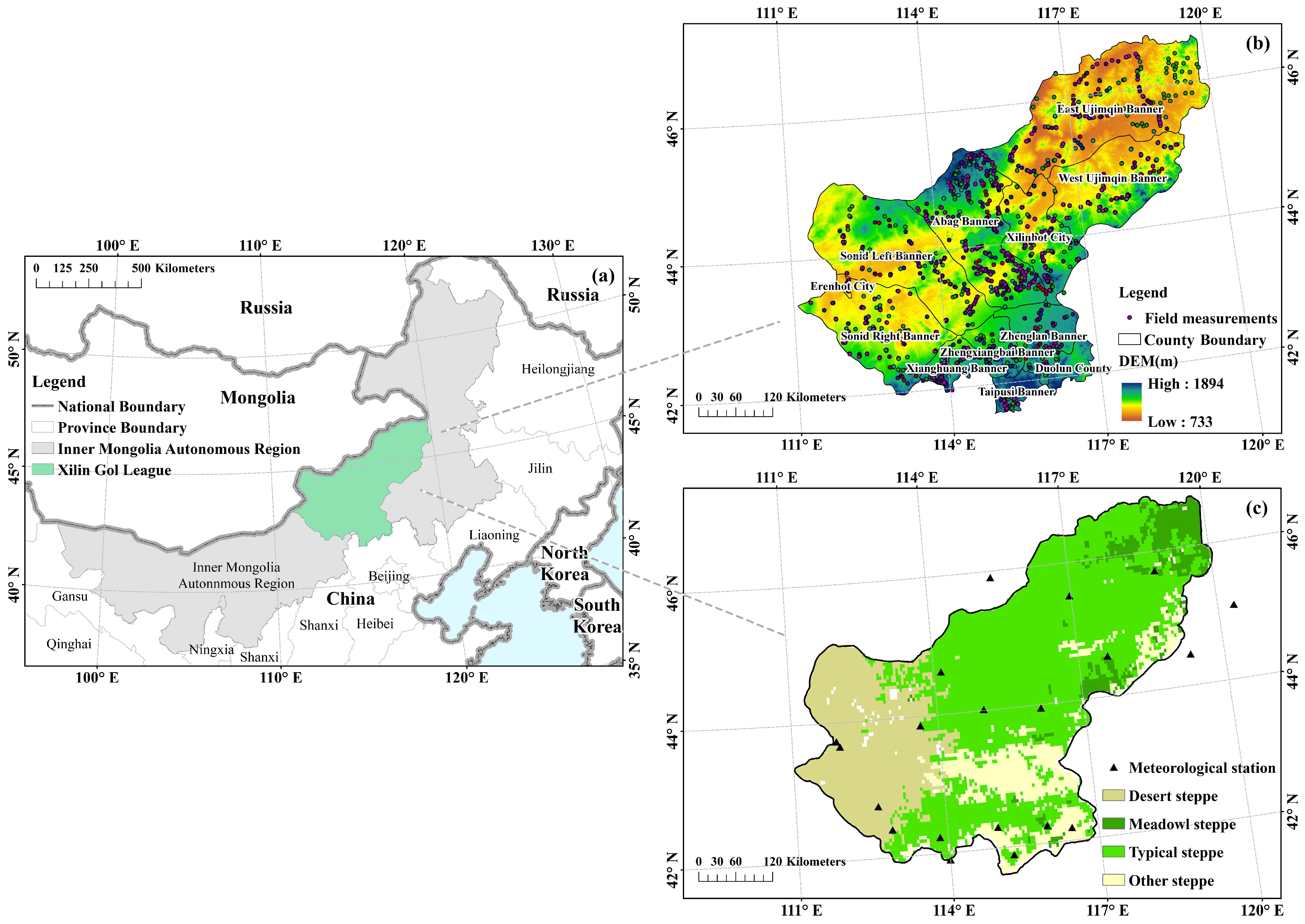
2.1. Study Area

Xilin Gol Grassland is located in the east-central area of Inner Mongolia (41°35′~46°46′N, 111°09′~119°58′E, Figure 1a), with a total area of 1.9 × 10⁵ km² and an altitude of 729~1939 m [29]. It belongs to the mid-temperate semi-arid to arid continental monsoon climate, with cold winters and hot summers. This region is influenced by different hydrothermal conditions and climatic environments, which results in various grassland types [30]. Typical grassland (TYG), meadow grassland (MEG), desert grassland (DRS) and other grasslands (OTHs) accounted for 58.7%, 6.8%, 24.1% and 10.4% of the total area, respectively (Figure 1c). The grassland of Xilin Gol is a significant livestock base in China, so the accurate estimation of grassland biomass is important for maintaining the balance of grass and livestock and realizing the sustainable development of grassland resources [30].

2.2. Data Sources

2.2.1. Field Measurement Data

The grass growth season of Xilin Gol League is mainly concentrated in April-September each year, in which August is the peak period of grass biomass [31]. From 2009 to 2015, we collected sample squares from the different grassland types in the administrative scope of the Xilin Gol League in August. To minimize the errors caused by the sample site selection, we selected the grassland communities far from roads or inside fences and those less disturbed by human activities. The spatial distribution of sample collection points is shown in Figure 1b. Sample squares 1 m × 1 m in size were collected evenly in each grassland type. The longitude, latitude and elevation of the samples were recorded, and the above-ground parts of the samples were mowed flush and finally dried in the laboratory to obtain the dry weight of the sample. The data were obtained from years of field measurements at the College of Geographical Sciences, Inner Mongolia Normal University.

2.2.2. Remote Sensing Data

To calculate the various vegetation indices, we used Landsat remote sensing satellite data with a spatial resolution of 30 m and a temporal resolution of 16 days from 2004 to 2015 (https://earthexplorer.usgs.gov/ (accessed on 23 May 2022)). These include Landsat 5 TM images from 2004 to 2011, Landsat 7 ETM+ images from 2012 and Landsat 8 OLI images from 2013 to 2015. The selected images with dates close to the sampling time for grass biomass and cloud cover of less than 20% included 16 images in the study area. The data were preprocessed by radiometric calibration, atmospheric correction, mosaic and cropping in the Google Earth Engine platform. The maximum synthetic method was used to calculate the monthly vegetation indices for each vegetation type.

We chose the 0–7 cm volumetric soil moisture of the Fifth-Generation ECMWF Reanalysis (ERA-5) product to analyze the effect of SM on grassland biomass. The daily 0.25° data are available at https://cds.climate.copernicus.eu/cdsapp/dataset/ (accessed on 19 May 2022), and were resampled to 30 m to be consistent with Landsat data.

In addition, evapotranspiration may affect the drought risk of grassland biomass. We downloaded the MODIS 8-day (MOD16A2) 500 m-resolution global evapotranspiration (ET) dataset (https://appeears.earthdatacloud.nasa.gov/task/area (accessed on 1 May 2022)) and resampled it to the same spatial resolution as the Landsat data.

Different soil types may affect the estimation of grassland biomass. Sand concentration in the surface soil (0–30 cm) dataset was downloaded from http://globalchange.bnu.edu.cn/research/soil (accessed on 13 May 2022), represented here as Sand. The spatial resolution was 500 m, and the data were resampled to 30 m as well.

2.2.3. Meteorological Station Dataset

We downloaded the meteorological data from the China Meteorological Data Sharing Service Network (http://cdc.cma.gov.cn (accessed on 13 May 2022)), including monthly maximum temperature (T_max), monthly minimum temperature (T_mix), monthly average precipitation, wind speed and sunshine hours. To improve the accuracy of meteorological data, we used the data of 13 meteorological stations in the study area and 3 surrounding meteorological stations for spatial interpolation, and the distribution of meteorological stations is shown in Figure 1c. The meteorological data were interpolated to a spatial resolution of 30 m using the Thin-Plate Spline method, which was consistent with the resolution of the Landsat data.

2.2.4. Socioeconomic Dataset

To analyze the effects of livestock quantity on grassland biomass and drought risk, we downloaded data on livestock numbers from the 2004–2015 Xilin Gol League Municipal Level Statistical Yearbook of Inner Mongolia Autonomous Region. We used the Thin-Plate Spline method for spatial differences.

2.3. Methods

2.3.1. Calculation of the Vegetation Index

The spectral index method is one of the basic methods for remote sensing inversion of surface parameters. It has certain mechanics and is easy to understand and use. This paper uses Landsat satellite data to calculate three vegetation indices, NDVI, EVI and FVC. The calculation formulas are shown in

Table 1. Calculation formulas of vegetation indices.

Name	Abbreviation	Formula	Reference
Normalized Difference Vegetation Index	NDVI	$\left(\mathit{NIR} - R\right)/\left(\mathit{NIR} + R\right)$	[32]
Enhanced Vegetation Index	EVI	$\frac{2.5\left(\mathit{NIR} - R\right)}{\left(\mathit{NIR} + 6 \times R + 7.5 \times \mathit{Blue} + 1\right)}$	[33]
Fractional Vegetation Cover	FVC	$\frac{\left(\mathit{NDVI} - {\mathit{NDVI}}_{\mathit{soil}}\right)}{\left({\mathit{NDVI}}_{\mathit{veg}} - {\mathit{NDVI}}_{\mathit{soil}}\right)}$	[34]

Notes: NIR, R and Blue are the reflectance of NIR, Red and Blue bands, respectively. The Blue, Red and NIR bands of Landsat 5 TM and Landsat 7 ETM+ are B1, B3 and B4, respectively, Landsat 8 OLI images in the Blue, Red and NIR corresponding to the B2, B4 and B5 bands, respectively. NDVI_veg and NDVI_soil are the NDVI values of pure vegetation pixels and pure bare soil pixels, respectively.

.

2.3.2. Random Forest

Random forest is a statistical learning method that was first proposed by Breiman in 2001 [35]. It is suitable for solving classification and regression problems. The principle of the random forest regression algorithm is to combine a large number of regression trees, each representing a set of conditions or constraints that are organized hierarchically and applied sequentially from the root to the leaves of the tree. Through repeated sampling, each sample is used to construct a decision tree. Training samples are continuously selected to minimize the sum of squared residuals until a complete tree is formed, and the final prediction is obtained by voting [36,37]. In this paper, eight elements (temperature (Tem), Prcp, SM, Lon, Sand1, NDVI, FVC and EVI) that may affect grassland biomass were selected as independent variables to build the model. The measured grassland biomass was used as the dependent variable. The process of building a grassland biomass estimation model in MATLAB software is as follows.

First, the original sample set is randomly divided into a training sample set and a test sample set, where the ratio of training samples to test samples is 7:3. Next, the training sample set is resampled by Bootstrap to obtain K training samples equal to the training sample set and generate K regression trees to form a random forest regression model (Equation (1)). At Bootstrap resampling, the probability of not being sampled is ${\left(1 - \frac{1}{N}\right)}^N$, when N→∞, ${\left(1 - \frac{1}{N}\right)}^N \approx 1/e \approx 0.368$, indicating that 36. 8% of the data are not extracted each time; these data are called Out of Bag (OOB) and can be used to estimate the prediction error [38].

$$h\left(x\right) = \frac{1}{N}{\sum }_{k = 1}^{K}h\left(x,{\theta }_k\right)$$

(1)

where x is the input vector, θ_k is the independent identically distributed random variable, K is the number of regression trees, and N is the number of samples in the training sample set. In this paper, we try to improve the accuracy of the model by gradually increasing the number of input variables and the combination of different variables, setting 500 regressions for 500 cycles of training and testing, respectively. The prediction average of all regression trees is used as the final prediction result.

$$H\left(x\right) = \frac{1}{K}{\sum }_{k = 1}^K{h}_k\left(x\right)$$

(2)

where H(x) denotes the average of the predicted values obtained from the K regression trees, and h_k(x) denotes the estimated value obtained from the kth regression tree trained on the training set.

2.3.3. Standardized Precipitation Evapotranspiration Index

We used the difference between precipitation (Prcp) and potential evapotranspiration (PET) to calculate the SPEI drought index. The difference between Prcp and PET for August of each year was calculated as follows:

$$D_i = Prc{p}_i - PE{T}_i$$

(3)

The calculated D values were aggregated at various time scales:

$$D_n^K = {\sum }_{i = 0}^{k - 1}\left(Prc{p}_{n - i} - PE{T}_{n - i}\right),n \ge k$$

(4)

where Prcp is precipitation, PET is the potential evapotranspiration, k is the aggregation time scale, and n is the final month [39]. $D_n^K$ is based on both the climatic water balance of the nth month and the water balance for the preceding k − 1 month. For example, the 3–month SPEI is constructed based on the sum of the D values from the two months preceding the current month [40].

To further analyze the relationship between the SPEI and grassland biomass at different time scales in this paper, SPEI–1, SPEI–3, SPEI–6, SPEI–12, SPEI–24 and SPEI–48 were calculated. They represent short-term (one–three months), medium-term (six months), medium-term (12 months) and long-term droughts (24 and 48 months), respectively.

2.3.4. Spearman Correlation Analysis

Spearman correlation analysis was used during the study period to calculate the correlation coefficients between grassland biomass and the SPEI in each August. The relationship between grass biomass and the SPEI at different time scales under drought conditions was analyzed. The correlation coefficient was calculated as follows:

$$r_{i,j} = \left({\mathit{biomass}}_i,\mathit{SPE}{I}_{i,j}\right)$$

(5)

$$i = 2004 - 2015;j = 1,3,6,12,24,48$$

(6)

$$\mathit{SPE}{I}_{i,j} \le -0.5$$

(7)

$$r_{\max \left(j\right)} = \mathit{max}\left(r_{i,j}\right),j = 8$$

(8)

where $r_{i,j}$ is the correlation coefficient, i is the years, j is the time scale of SPEI, and ${\mathit{biomass}}_i$ and $\mathit{SPE}{I}_{i,j}$ represent the corresponding grassland biomass and SPEI data when $\mathit{SPE}{I}_{i,j} \le -0.5$. $r_{\mathit{max}\left(j\right)}$ is the maximum correlation coefficient between biomass and the SPEI at different time scales calculated by the MVC method [41,42].

2.3.5. Risk Assessment

Based on the theory of risk formation, the risk is the product of disasters and vulnerabilities [42]. Drought disaster is mainly determined by drought intensity and drought frequency, while drought vulnerability (DV) is the vulnerability of drought-related exposure factors to adverse impacts [43]. Vulnerability includes sensitivity and adaptation of grassland biomass to drought. The quantitative assessment of drought risk was quantified for different grassland types based on the response of the grassland ecosystems to climate change. The DR was calculated as follows:

$$DR = \frac{1}{12}{\sum }_{i = 1}^{n = 12}D{H}_i \times D{V}_i$$

(9)

where i represents August of each year during the study period from 2004 to 2015. Due to the different biomass responses to drought stress in different years, the DH and DV values for August of each year were calculated.

This paper uses the SPEI for drought identification and the probability density function (PDF) to calculate drought disasters [25]. The DH was calculated as follows:

$$\mathit{DH} = {\int }_{-3.5}^{-0.5}\mathit{SPEI} \times f\left(\mathit{SPEI}\right)$$

(10)

where $\mathit{SPEI}$ represents drought frequency and $f\left(\mathit{SPEI}\right)$ represents drought intensity.

The vulnerability of grassland biomass to drought can be expressed as follows:

$$D{V}_i = D{S}_i \times D{A}_i$$

(11)

where $D{V}_i$ represents the vulnerability of grassland biomass to drought. Higher values of $D{V}_i$ indicate a higher vulnerability of biomass to drought.

Since many factors influence drought sensitivity and vulnerability, we use the ratio of the rate of change in the grassland biomass to the rate of change in SPEI to express the sensitivity of grassland biomass [43,44]. Furthermore, this paper quantitatively describes the drought sensitivity of grassland biomass. Defined as the ratio of the biomass change rate to the SPEI change rate under drought conditions (SPEI$\le -0.5$), the DS was calculated as follows:

$$\mathit{DS} = \underset{∆\mathit{SPEI}\to 0}{\mathit{lim}}\left(\frac{∆\mathit{Biomass}/\overline{\mathit{Biomass}}}{∆\mathit{SPEI}/\overline{\mathit{SPEI}}}\right)=\frac{\partial \mathit{Biomass}}{\partial \mathit{SPEI}}\times \frac{\overline{\left|\mathit{SPEI}\right|}}{\overline{\mathit{NVDI}}}$$

(12)

where DS is the sensitivity of grassland biomass to drought. The larger the DS value, the higher the sensitivity of biomass to drought. When DS < 0, it can be considered that drought may not be the main limiting factor for grassland biomass.

Adaptation represents a response of grasslands to potential losses caused by drought and changes to maintain the stability of grassland ecosystems [45]. The DA was calculated as follows:

$$DA = \frac{1}{n}{\sum }_{i = 1}^n\left|\frac{\left({\mathit{Biomass}}_i-{\mathit{Biomass}}_{\mathit{mean}}\right)/{\mathit{Biomass}}_{\mathit{mean}}}{{\mathit{SPEI}}_i-{\mathit{SPEI}}_{\mathit{mean}}}\right|,\mathit{SPEI} \le -0.5$$

(13)

where DA is the adaptation of grasslands to drought, and a higher DA value indicates lower adaptability. ${\mathit{Biomass}}_i$ and $\mathit{SPE}{I}_i$ are long-time series data of biomass and SPEI under drought conditions, respectively. ${\mathit{Biomass}}_{\mathit{mean}}$ and $\mathit{SPE}{I}_{\mathit{mean}}$ represent the mean values of biomass and the SPEI during the study period, respectively.

SPEI values were calculated for six time scales in this study, and their correlations with grassland biomass were calculated separately. The highest correlation was selected for calculating drought hazard, sensitivity and adaptation of the grassland biomass. To quantify the DR, DH, DS and DA were first standardized in the calculation, yielding values distributed in the range of 0–1. The calculation formula is as follows:

$$x^{\prime } = \frac{x}{x_{\mathit{max}}}$$

(14)

where x represents all pixel values, and $x_{\mathit{max}}$ represents the maximum value of image elements in the same variable.

2.3.6. Structural Equation Modeling (SEM)

SEM is a statistical method for analyzing the relationship between variables based on the covariance matrix of the variables. These relationship strengths accurately represent the cause and effect of the process being studied. SEM, unlike other methods of statistical modeling, allows the inclusion of all interactions and interdependencies that accompany a given process or phenomenon [46]. Since DR is calculated from the product of DV and DH, there may be some uncertainty. To analyze the effects of various factors on the drought risk of different grassland types and to explore the intrinsic links between the factors, a pathway analysis of drought risk for different grassland types of biomasses was conducted using SEM (Figure 2).

3. Results

3.1. Establishing an Estimation Model for Grassland Biomass in Xilin Gol League Based on a Random Forest Algorithm

In this paper, eight factors (Tem, Prcp, SM, Lon, Sand1, NDVI, FVC and EVI) that may affect the estimation of grassland biomass were selected from the aspects of meteorological, soil and vegetation factors. The random forest algorithm was used to improve the accuracy of model estimation by gradually increasing the number of input variables and the combinations between variables. The accuracy of the models established by different input variables is shown in Figure 3a. The accuracy of the model improved significantly with an increase in the number of input variables. The highest model accuracy was achieved when four variables were input. In this study, the corresponding input variables were NDVI, Prcp, SM and Lon, and the model accuracy is shown in Figure 3b, as R = 0.90 and RMSE = 0.09 kg/m². With further increases in the number of input variables, R remained between 0.88 and 0.89, without significant improvement in model accuracy. Based on the principles of high model accuracy, low input parameters and ease of use, NDVI, Prcp, SM and Lon were selected as the input variables for establishing a grassland biomass estimation model and performing spatial inversion of the grassland biomass.

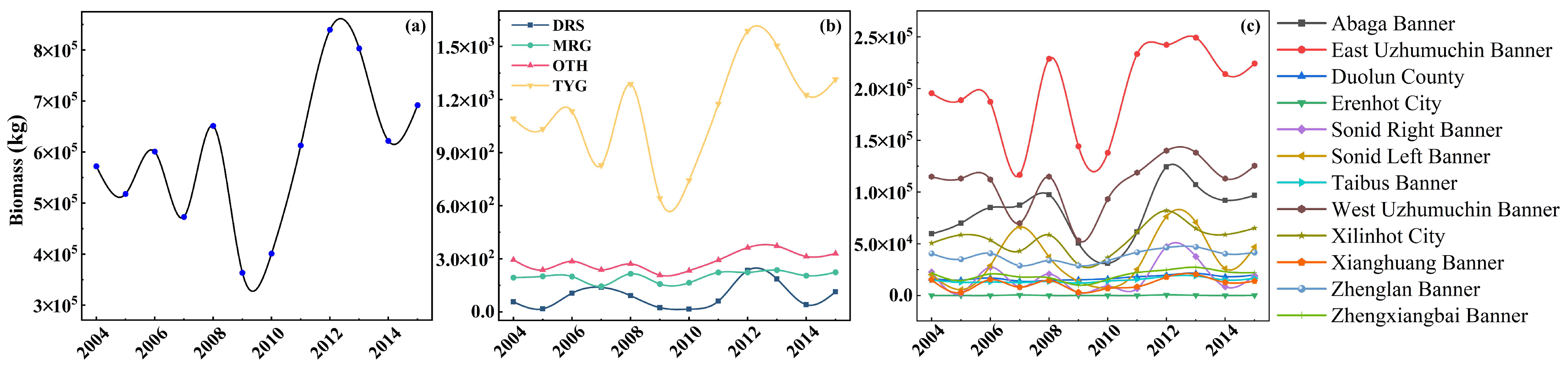
3.2. Temporal and Spatial Variation in Grassland Biomass

3.2.1. Temporal Variation in Grassland Biomass

Figure 4a shows that the overall grassland biomass in Xilin Gol League increased from 2004 to 2015. The first peak of grassland biomass was reached in 2008 at 6.51 × 10⁵ kg, followed by a significant decrease to the lowest value in 2009 at 3.63 × 10⁵ kg. After 2009, grassland biomass gradually recovered at a rate of 1.59 × 10⁴ kg/year. In 2012, the grassland biomass peaked again at 8.40 × 10⁵ kg. Subsequently, the grassland biomass began to decline slowly and stabilized at 6.9 × 10⁵ kg during 2014–2015.

Figure 4b shows the interannual variation in biomass in different grassland types. As the dominant grassland of the Xilin Gol League, TYG is widely distributed and has the highest biomass. Its interannual variation trend is similar to that of the overall grassland biomass in the Xilin Gol League. During the study period, the two peaks appeared in 2008 (1.29 × 10³ kg) and 2013 (1.59 × 10³ kg). Meadow grassland had the second highest biomass, and desert grassland had the lowest biomass. OTH biomass tended to stabilize, and remained around 262.51 kg.

Among the various banners and counties, East Ujimqin Banner and West Ujimqin Banner had the most grassland biomass (Figure 4c). Their grassland biomass trends were similar, decreasing year by year before 2007 and increasing significantly after 2007 to a peak in 2008, with grassland biomasses of 2.83 × 10⁵ kg and 1.19 × 10⁵ kg, respectively. Grassland biomass gradually increased after 2009. Erlianhot City, Sunit Left Banner and Sunit Right Banner had less grassland biomass. Their annual average biomass levels were 139.42 kg, 3.54 × 10⁴ kg and 1.76 × 10⁴ kg, respectively, and their grassland biomass variations tended to be stable.

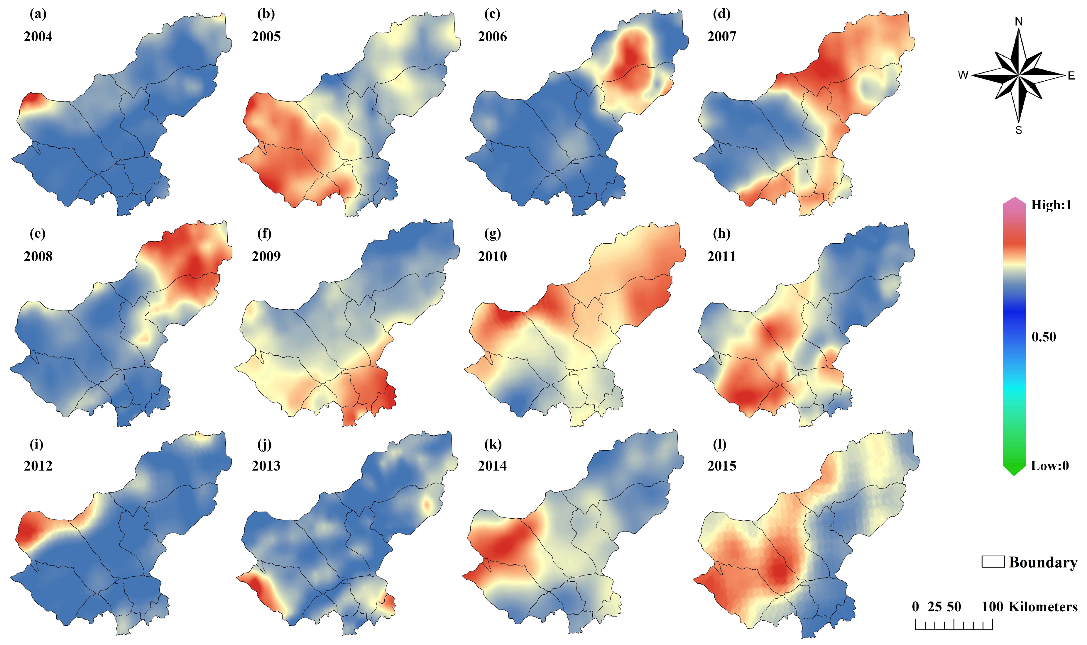
3.2.2. Spatial Variation in Grassland Biomass

The spatial distribution of grassland biomass (Figure 5) indicates that the grassland biomass in Xilin Gol League is generally high in the east and low in the west. The average annual grass biomass in the study area over 12 years was 6.0 × 10⁵ kg, with significant spatial differences in biomass for each grassland type. The average annual grass biomass of TYG reached 1.13 × 10³ kg, mainly in the southwest of East Ujumqin, the northwest of West Ujumqin Banner, Xilinhot City and most areas of Abaga Banner. The southern part of East Ujimqin and the northeastern part of West Ujimqin Banner are areas with high grassland biomass per unit area, mostly 0.15~0.30 kg/m². The northern part of Xilinhot City and the central and western parts of Abaga Banner are areas with a low grassland biomass of 0~0.15 kg/m². Figure 5d shows that grass biomass was lower in the western region of East Urumqi in 2007, unlike in other years, and then remained relatively stable for the rest of the years.

MEG is located in the northeastern part of East Ujimqin and the southwestern part of West Ujimqin Banner, with an average annual grass biomass of 177.59 kg. MEG has the highest grassland biomass in the entire Xilin Gol. Figure 5h–k shows that the meadow grassland biomass per unit area is mostly 0.45 to 0.75 kg/m². In 2010, the meadow grass-land biomass decreased significantly to 0.15~0.30 kg/m², and then it recovered year by year.

DRS is the area with the lowest grassland biomass. It is located in the western part of Xilin Gol League, covering Erlianhot City, Sunit Left Banner and Sunit Right Banner, with an average annual grassland biomass of 72.88 kg. After 2006, areas of 0.15~0.30 kg/m² appeared sporadically, and from 2009 to 2011, the grassland biomass per unit area in most areas was 0~0.15 kg/m². In 2012, the biomass of desert steppe grassland was the highest, ranging from 0.15 to 0.30 kg/m² in most areas.

OTH is mainly distributed in Taipusi Banner, Duolun County, Zhengxiangbai Ban-ner, north of Zhenglan Banner, Sunite Zuo Banner, south of Xilinhot City in Abaga Banner and east of West Ujimqin Banner. The biomass levels in these areas have been relatively stable, around 0.15~0.30 kg/m², with insignificant changes over the years.

3.3. Optimal SPEI Time Scale Selection for Drought Risk Assessment of Grassland Biomass

The spatial distribution of the correlation between grassland biomass and the SPEI at different time scales is shown in Figure 6. Regions with a high correlation show variability depending on the time scale of the SPEI. The regions with a high correlation (R > 0.5) between SPEI–3 and SPEI–6 and grassland biomass were mainly distributed in the northwestern part of East Ujumqin Banner, the central and northern parts of Abaga Banner and the southern part of Xilinhot City, where the main grassland types are TYG. The areas with a high correlation between SPEI–48 and grassland biomass were in southwestern East and West Ujimqin Banner. A statistical analysis was performed on the correlation and significance of the different grassland types (Figure 6 and Figure 7). Among the SPEI drought indicators on the six time scales, the area of SPEI–3 was positively correlated with grassland biomass, accounting for 91.67% of the total study area, and it had the highest correlation with grassland biomass. Figure 7a shows that with the increase in the SPEI time scale, the correlation between the biomasses of different grassland types and SPEI showed an increase at first and then a decreasing trend. The correlation peaked at SPEI–3, and significant area statistics showed similar trends. Among the various grassland types, TYG biomass had the highest correlation with SPEI–3, and the area with significance was up to 80%. Therefore, this study selected SPEI–3 as the drought assessment index for grassland biomass.

3.4. Drought Risk Assessment of Different Grassland Types

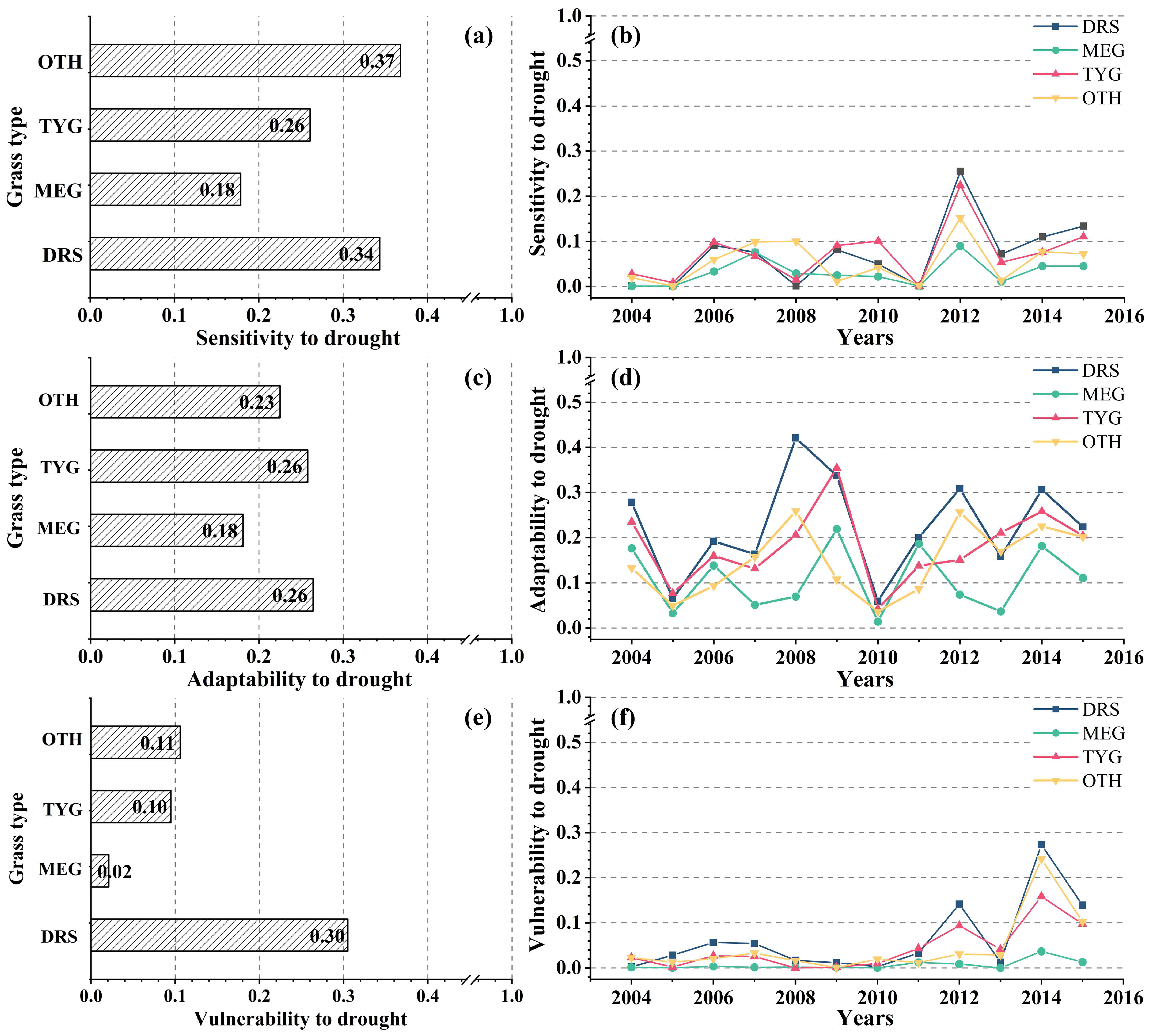
3.4.1. Drought Hazard Assessment of Different Grassland Types

The spatial distribution of grassland biomass drought hazards is shown in Figure 8. Over time, the area and scope of the drought suffered by the grassland of the Xilin Gol League have changed. Sunit Left Banner and Sunit Right Banner were the regions with the highest frequency of drought disasters over the 12 years, and the frequency of drought disasters in East Urumqi, West Urumqi and Abaga Banner was low. Figure 9a shows that the drought disasters of different grassland types were not significantly different, and the DH was concentrated between 0.83 and 0.85. The degree of drought of the various grassland types was in the order of: DRS > MEG > OTH > TYG. The temporal variations in drought hazards in different grassland types are shown in Figure 9. The drought hazards of various grassland types showed fluctuating changes. Various grassland types suffered severe drought disasters in 2005, 2007, 2010 and 2014, but fewer drought hazards in 2004, 2006, 2008 and 2013.

3.4.2. Drought Vulnerability Assessment of the Different Grassland Types

The results of the drought sensitivity analysis (Figure 10a) revealed differences in the sensitivity of different grasslands to drought. The sensitivity of TYG reached up to DS = 0.37, followed by DRS at 0.34, while MEG was the lowest at 0.18. This result indicates that OTH is more vulnerable when drought occurs. Figure 10b shows that the drought sensitivity of grasslands alternated over time, with higher sensitivity appearing in 2006, 2010 and 2012. In particular, the sensitivity of various grassland types reached their historical peaks in 2012 and then showed downward trends, while the values in 2005, 2008 and 2011 were relatively low.

In general, vegetation sensitivity and adaptation show opposite trends, with grasslands that are less sensitive to drought having higher adaptation. Figure 10c shows that the adaptation of DRS to drought was the highest among the various grassland types, reaching DA = 0.26, while the lowest adaptation was DA = 0.26 for MEG. These results indicate that MEG is less adaptable and more vulnerable to the effects of drought. The temporal variation in drought adaptation in different grasslands (Figure 10d) shows that the adaptability of various grasslands to drought also changed in an alternating fashion. Higher adaptability was found in 2009, 2012 and 2015, while poor adaptability was seen in 2005 and 2010.

The analysis of drought vulnerability of different grasslands (Figure 10e) showed that DRS had the highest drought vulnerability, followed by OTH and TYG, and MEG had the lowest. The drought vulnerability of various grasslands was relatively stable until 2011 (Figure 10f), maintaining values between 0 and 0.06, with significant periods of vulnerability in 2012 and 2014, followed by a gradual improvement.

3.4.3. Drought Risk Assessment of Different Grassland Types

The numerical distributions of drought risk and vulnerability were relatively similar (Figure 11). DRS drought risk was the highest, with a DR of 0.30, while OTH and TYG were comparable in risk. The minimum drought risk was 0.02 for MEG. Figure 11b shows that drought risk was relatively low for all grassland types until 2011, fluctuating between 0 and 0.06, while 2012 and 2014 were two peak periods for various grassland drought risks, followed by a gradual recovery.

3.5. Analysis of Drought Risk Drivers

SEM pathway analysis shows that Tem, Prcp, SM and ET affected the drought risk of different grassland types of biomasses in Xilin Gol League to varying degrees (Figure 12). The coefficients of the effects of the factors on drought risk mostly showed positive direct effects. The highest action coefficient was found for Tem in TYG (0.592), followed by Prcp (0.519). ET had a direct negative impact on DR (−0.565), while a direct significant positive effect was found between ET and NDVI with an action coefficient of 0.675. Prcp and ET in MEG presented negative direct impacts on drought risk, with effect coefficients of −0.665 and −0.650, respectively. Among the factors showing a positive direct significant effect, SM had the highest coefficient of action of 0.781, followed by Tem at 0.587. The highest action coefficient of ET on DR in DRS was 0.660. Prcp and Tem in OTH illustrated negative direct and significant effects on DR, with effect coefficients of −0.687 and −0.602, respectively, similar to the performance of Prcp in MEG. The highest path coefficient of 0.632 was found in SM. ET showed a positive and significant effect on the NDVI in all grassland types, with the highest coefficient being 0.769 for DRS and 0.675 for TYG. Prcp also exhibited a positive effect on SM across grassland types, with the highest OTH effect coefficient being 0.696 and the lowest DRS being 0.223.

4. Discussion

4.1. Model Rationalization and Evaluation Results

Grassland biomass estimation models based on machine learning algorithms have been widely applied, and they have proven to be effective in improving biomass estimation accuracy [47,48,49]. In this study, a random forest regression algorithm was used to eliminate the influences of factors that have little impact on grassland biomass by constantly adjusting the number of input variables and changing the combination of variables, which effectively improved the accuracy of the model while reducing the computational effort. Our findings indicate that when the input variables were the NDVI, Prcp, SM and Lon, the accuracy of the model reached its highest level, with R = 0.90 and RMSE = 0.09kg/m². These results were compared with the biomass estimation model developed by Liu et al. [50] in Inner Mongolian grasslands, where R increased by 0.42. The NDVI has been used as an indicator of vegetation growth since the early 1970s [51]. Many studies have demonstrated that the NDVI is significantly correlated with grassland biomass [52,53,54]. In addition, Xilin Gol League is located in an arid and semi-arid area, and the temperature in August is relatively stable (18.6 °C~21.7 °C). Therefore, Prcp becomes the main meteorological factor affecting the growth of grassland, which is consistent with the results of previous research [55]. The east–west longitudinal range of Xilin Gol League grassland spans 9°. To improve the accuracy of the model calculations, longitude was selected as the characteristic variable affecting grassland biomass. Compared with models that do not consider the effect of longitude change, the R increased by 0.006, similar to the findings of Yang et al. in Sanjiangyuan [56].

4.2. Analysis of Grassland Biomass and Drivers of Drought Risk

Results of the highest correlation of grassland biomass with SPEI–3 are consistent with the correlation between the SPEI and NDVI found by Li et al. in the northeastern region [20]. The reason for high drought risk DRS and low MEG among the four grassland types may be that the desert grasslands are composed of xerophytic clumps of small grasses and small semi-shrubs, mainly in Sunit Left Banner, Sunit Right Banner and Erlianhot City. These vegetation types usually have low vegetation coverage, or even bare ground, combined with less precipitation, resulting in the highest risk of drought in the desert grasslands [57]. The meadow grassland is mainly located in the northeastern part of East Urumqi and southeastern part of West Urumqi, and consists of perennial clump grasses and rhizomatous grasses. The vegetation has a suitable height, good growth and high vegetation cover. In addition, the region has high precipitation and soil moisture, resulting in a low risk of MEG drought.

The combined effects of climate change and human activities are the external drivers of vegetation dynamics and spatial heterogeneity [58]. In the DR calculations for all grassland types, the path coefficients from meteorological elements to DR were larger, indicating that climatic factors contribute more to drought risk. Previous studies have shown that climate change can significantly affect the drought risk of vegetation [59]. The results of structural equation modeling indicate that the drivers of drought risk show variability across grassland types. Among the drought risk drivers of TYG, the path coefficients of Tem, Prcp, ET and SM were all >0.5, with Tem reaching a maximum of 0.592. This is mainly because Xilin Gol is located in an arid and semi-arid region [55]; the increased temperature increases the risk of drought in TYG, consistent with the results of Noah S. Diffenbaugh et al. [60,61]. Prcp and SM mainly drive drought risk in MEG. Soil moistures in East Ouzhuqin are higher and less affected by meteorological factors such as temperature and precipitation, so the root system of MEG is well-developed and can easily absorb water from the soil for vegetation growth, resulting in more resilience to short-term drought events. ET is the main driver of drought risk in DRS. Due to persistent desertification, vegetation cover in DRS is reduced, soil water content become low [60,62], and transpiration from vegetation is reduced, which results in lower evapotranspiration from DRS, leading to frequent DRS drought events in arid and semi-arid regions [63]. Extreme drought events happened in some regions of DRS, with less precipitation in desert grasslands and increased temperatures, thus exacerbating the risk of drought in DRS [64]. OTH contains a variety of mixed pixels, including farmland, shrubs and build-up. The grassland pixels occupy a small proportion and are seriously affected by human beings. The impact of meteorological elements on drought risk is not obvious enough, or even negatively correlated [65]. In addition, severe drought events in arid regions imply a deterioration in climate stability, which may also lead to weakened crop resistance and increased vulnerability to climate change. The drought risk intensity depends mainly on the adaptation and sensitivity of vegetation to external drivers. When the increase in adaptability exceeds sensitivity, the driver shows a positive effect. Therefore, the analysis of climate change and human activity provides a good picture of the relationships between risk and the various drivers.

4.3. Limitations

Based on the IPCC definition of drought risk, this study proposes a method for calculating grassland biomass and risk assessment, but some shortcomings still need to be improved. First, the accuracy of the grassland biomass estimation model based on a random forest algorithm reached R = 0.90. Due to the small number and uneven distribution of meteorological stations in this area, errors in Landsat image dates and biomass sampling times may reduce the accuracy of biomass estimation models. Despite imposing a threshold of cloud coverage of less than 20% of the Landsat images, there was still an impact on the model accuracy. In addition, the SPEI is calculated by spatial interpolation, so there is some error in the spatial resolution. In future studies, we will extend the time scale and select remote sensing images that were obtained closer to the sampling dates with a higher spatial resolution in order to improve the accuracy of the model estimations. The spatial heterogeneity of grassland biomass is influenced by various factors such as climate change, human activities, soil, groundwater and fire. Therefore, the present study is insufficient as it considers only the number of livestock as an anthropogenic activity factor, and more detailed and comprehensive studies are needed.

5. Conclusions

In this study, we developed a model for estimating grassland biomass in Xilin Gol based on multi-source data using the random forest method to analyze its spatial and temporal variation characteristics. The drought risk of grassland biomass was also ana-lyzed using the SPEI drought index and SEM to study the drivers affecting drought risk in different grassland types of biomasses. The results lead to three main conclusions:

(1)

Among the eight selected variables affecting grassland biomass, the NDVI, Prcp, SM and Lon were combined as input variables, and the highest model accuracy for estimating biomass was R = 0.90 and RMSE = 0.09 kg/m². During the study period, the biomass of typical grassland was the highest, and the biomass of desert grassland was the lowest, showing a spatial distribution that gradually decreases from northeast to southwest.

(2)

Drought risk to grassland biomass in the Xilin Gol League shows a fluctuating trend over time. The years 2012 and 2014 had the highest drought risk during the study period. There were differences in drought risk among grassland types, among which the highest drought risk was found in desert grassland (DR = 0.30) and the lowest in meadow grassland (DR = 0.02).

(3)

The effects of various factors on drought risk differed depending on the grassland type. Tem mainly drives TYG drought risk, while SM greatly impacts drought risk in MEG. ET has a relatively high contribution to the drought risk of DRS. Drought risks in the other grasslands are more sensitive to Prcp.

References

1. Zhao, A.; Zhang, A.; Liu, X.; Cao, S. Spatiotemporal changes of normalized difference vegetation index (NDVI) and response to climate extremes and ecological restoration in the Loess Plateau, China. Theor. Appl. Climatol. 2018, 132, 555–567. [Google Scholar]
2. Dai, A. Increasing drought under global warming in observations and models. Nat. Clim. Chang. 2013, 3, 52–58. [Google Scholar]
3. He, B.; Liu, J.; Guo, L.; Wu, X.; Xie, X.; Zhang, Y.; Chen, C.; Zhong, Z.; Chen, Z. Recovery of Ecosystem Carbon and Energy Fluxes From the 2003 Drought in Europe and the 2012 Drought in the United States. Geophys. Res. Lett. 2018, 45, 4879–4888. [Google Scholar]
4. Huang, L.; He, B.; Chen, A.; Wang, H.; Liu, J.; Lű, A.; Chen, Z. Drought dominates the interannual variability in global terrestrial net primary production by controlling semi-arid ecosystems. Sci. Rep. 2016, 6, 24639. [Google Scholar] [CrossRef] [PubMed] [Green Version]
5. Huang, L.; He, B.; Han, L.; Liu, J.; Wang, H.; Chen, Z. A global examination of the response of ecosystem water-use efficiency to drought based on MODIS data. Sci. Total Environ. 2017, 601–602, 1097. [Google Scholar]
6. He, B.; Lü, A.; Wu, J.; Lin, Z.; Ming, L. Drought hazard assessment and spatial characteristics analysis in China. J. Geogr. Sci. 2011, 21, 235–249. [Google Scholar] [CrossRef]
7. Qu, Y.; Zhao, Y.; Ding, G.; Chi, W.; Gao, G. Spatiotemporal patterns of the forage-livestock balance in the Xilin Gol steppe, China: Implications for sustainably utilizing grassland-ecosystem services. J. Arid Land 2021, 13, 135–151. [Google Scholar]
8. You, L.Q.; Ping, T.Y. The effects of land use change on the eco-environmental evolution of farming-pastoral region in Northern China:With an emphasis on Duolun County in Inner Mongolia. Acta Ecol. Sin. 2003, 23, 1025–1030. [Google Scholar]
9. Lu, D. The potential and challenge of remote sensing-based biomass estimation. Int. J. Remote Sens. 2006, 27, 1297–1328. [Google Scholar]
10. Iftikhar, A.; Fiona, C.; Edward, D.; Brian, B.; Stuart, G. Satellite remote sensing of grasslands: From observation to management—A review. J. Plant Ecol. 2016, 9, 649–671. [Google Scholar]
11. Prasad, R.; Pandey, A.; Singh, K.P.; Singh, V.P.; Mishra, R.K.; Singh, D. Retrieval of spinach crop parameters by microwave remote sensing with back propagation artificial neural networks: A comparison of different transfer functions. Adv. Space Res. 2012, 50, 363–370. [Google Scholar]
12. Wang, D.C.; Wang, J.H.; Jin, N.; Wang, Q.; Huang, F. ANN-based wheat biomass estimation using canopy hyperspectral vegetation indices. Trans. Chin. Soc. Agric. Eng. 2008, 24, 196–201. [Google Scholar]
13. Li, Q.; Chen, L.; Xu, Y. Drought risk and water resources assessment in the Beijing-Tianjin-Hebei region, China. Sci. Total Environ. 2022, 832, 154915. [Google Scholar] [CrossRef] [PubMed]
14. Jin, L.; Zhang, J.; Wang, R.; Zhang, M.; Bao, Y.; Guo, E.; Wang, Y. Analysis for Spatio-Temporal Variation Characteristics of Droughts in Different Climatic Regions of the Mongolian Plateau Based on SPEI. Sustainability 2019, 11, 5767. [Google Scholar]
15. Hao, Z.; Singh, V.P. Drought characterization from a multivariate perspective: A review. J. Hydrol. 2015, 527, 668–678. [Google Scholar] [CrossRef]
16. Mckee, T.B.; Doesken, N.J.; Kleist, J. The Relationship of drought frequency and duration to time scales. In Proceedings of the 8th Conference on Applied Climatology, Anaheim, CA, USA, 17–22 January 1993; pp. 179–183. [Google Scholar]
17. Vousdoukas, M.I.; Mentaschi, L.; Voukouvalas, E.; Bianchi, A.; Dottori, F.; Feyen, L. Climatic and socioeconomic controls of future coastal flood risk in Europe. Nat. Clim. Chang. 2018, 8, 776–780. [Google Scholar] [CrossRef]
18. Du, L.; Tian, Q.; Yu, T.; Meng, Q.; Jancso, T.; Udvardy, P.; Huang, Y. A comprehensive drought monitoring method integrating MODIS and TRMM data. Int. J. Appl. Earth Obs. Geoinf. 2013, 23, 245–253. [Google Scholar]
19. Dai, A. Drought under global warming: A review. Wiley Interdiscip. Rev. Clim. Chang. 2011, 2, 45–65. [Google Scholar]
20. Li, K.; Tong, Z.; Liu, X.; Zhang, J.; Tong, S. Quantitative assessment and driving force analysis of vegetation drought risk to climate change:Methodology and application in Northeast China. Agric. For. Meteorol. 2019, 282–283, 107865. [Google Scholar]
21. Xu, H.J.; Wang, X.P.; Zhao, C.Y.; Yang, X.M. Diverse responses of vegetation growth to meteorological drought across climate zones and land biomes in northern China from 1981 to 2014. Agric. For. Meteorol. 2018, 262, 1–13. [Google Scholar] [CrossRef]
22. Vicente-Serrano, S.M.; Gouveia, C.; Camarero, J.J.; Beguería, S.; Trigo, R.; López-Moreno, J.I.; Azorín-Molina, C.; Pasho, E.; Lorenzo-Lacruz, J.; Revuelto, J. Response of vegetation to drought time-scales across global land biomes. Proc. Natl. Acad. Sci. USA 2013, 110, 52–57. [Google Scholar] [PubMed] [Green Version]
23. Wilhite, D.A. Drought as a Natural Hazard: Concepts and Definitions. 2000. Available online: http://digitalcommons.unl.edu/droughtfacpub (accessed on 26 September 2022).
24. Wisner, B.; Blaikie, P.; Cannon, T.; Davis, I. At Risk: Natural Hazards, People’s Vulnerability and Disasters; Routledge: London, UK, 2014. [Google Scholar]
25. Zhang, Q.; Zhang, J.; Wang, C. Risk assessment of drought disaster in typical area of corn cultivation in China. Theor. Appl. Climatol. 2017, 128, 533–540. [Google Scholar]
26. Pachauri, R.; Meyer, L. Climate Change 2014: Synthesis Report. Contribution of Working Groups I, II and III to the Fifth Assessment Report of the Intergovernmental Panel on Climate Change. 2014. Available online: https://epic.awi.de/id/eprint/37530/ (accessed on 26 September 2022).
27. Yang, X.; Li, Y.P.; Huang, G. A maximum entropy copula-based frequency analysis method for assessing bivariate drought risk: A case study of the Kaidu River Basin. J. Water Clim. Chang. 2022, 13, 175–189. [Google Scholar]
28. Zhang, L.; Chu, Q.Q.; Jiang, Y.L.; Fu, C.; Lei, Y.D. Impacts of climate change on drought risk of winter wheat in the North China Plain. J. Integr. Agric. 2021, 20, 2601–2612. [Google Scholar]
29. Tong, C.; Wu, J.; Yong, S.-p.; Yang, J.; Yong, W. A landscape-scale assessment of steppe degradation in the Xilin River Basin, Inner Mongolia, China. J. Arid Environ. 2004, 59, 133–149. [Google Scholar] [CrossRef]
30. Wang, Z.; Yu, Q.; Guo, L. Quantifying the impact of the grain-for-green program on ecosystem health in the typical agro-pastoral ecotone: A case study in the Xilin Gol league, Inner Mongolia. Int. J. Environ. Res. Public Health 2020, 17, 5631. [Google Scholar] [CrossRef]
31. Javed, T.; Li, Y.; Feng, K.; Ayantobo, O.O.; Ahmad, S.; Chen, X.; Rashid, S.; Suon, S. Monitoring responses of vegetation phenology and productivity to extreme climatic conditions using remote sensing across different sub-regions of China. Environ. Sci. Pollut. Res. 2021, 28, 3644–3659. [Google Scholar]
32. Jiang, R.; Wang, P.; Xu, Y.; Zhou, Z.; Luo, X.; Lan, Y.; Zhao, G.; Sanchez-Azofeifa, A.; Laakso, K. Assessing the operation parameters of a low-altitude UAV for the collection of NDVI values over a paddy rice field. Remote Sens. 2020, 12, 1850. [Google Scholar] [CrossRef]
33. Matsushita, B.; Yang, W.; Chen, J.; Onda, Y.; Qiu, G. Sensitivity of the enhanced vegetation index (EVI) and normalized difference vegetation index (NDVI) to topographic effects: A case study in high-density cypress forest. Sensors 2007, 7, 2636–2651. [Google Scholar] [CrossRef] [Green Version]
34. Liu, Q.; Zhang, T.; Li, Y.; Li, Y.; Bu, C.; Zhang, Q. Comparative analysis of fractional vegetation cover estimation based on multi-sensor data in a semi-arid sandy area. Chin. Geogr. Sci. 2019, 29, 166–180. [Google Scholar]
35. Breiman, L. Random forests. Mach. Learn. 2001, 45, 5–32. [Google Scholar] [CrossRef] [Green Version]
36. Zhou, X.; Zhu, X.; Dong, Z.; Guo, W. Estimation of biomass in wheat using random forest regression algorithm and remote sensing data. Crop J. 2016, 4, 212–219. [Google Scholar]
37. Chan, J.C.-W.; Paelinckx, D. Evaluation of Random Forest and Adaboost tree-based ensemble classification and spectral band selection for ecotope mapping using airborne hyperspectral imagery. Remote Sens. Environ. 2008, 112, 2999–3011. [Google Scholar]
38. Gong, H.; Sun, Y.; Shu, X.; Huang, B. Use of random forests regression for predicting IRI of asphalt pavements. Constr. Build. Mater. 2018, 189, 890–897. [Google Scholar] [CrossRef]
39. Potopová, V.; Stepanek, P.; Mozny, M.; Soukup, J. Performance of the standardised precipitation evapotranspiration index at various lags for agricultural drought risk assessment in the Czech Republic. Agric. For. Meteorol. 2015, 202, 26–38. [Google Scholar]
40. Begueria-Portugues, S.; Vicente-Serrano, S.; Angulo-Martínez, M.; López-Moreno, J.; EIKenawy, A. The Standardized Precipitation-Evapotranspiration Index (SPEI): A multiscalar drought index. In Proceedings of the 10th EMS Annual Meeting, Zürich, Switzerland, 13–17 September 2010; p. EMS2010-2562. [Google Scholar]
41. Zhou, Q.; Luo, Y.; Zhou, X.; Cai, M.; Zhao, C. Response of vegetation to water balance conditions at different time scales across the karst area of southwestern China—A remote sensing approach. Sci. Total Environ. 2018, 645, 460–470. [Google Scholar]
42. Zhao, A.; Zhang, A.; Cao, S.; Liu, X.; Liu, J.; Cheng, D. Responses of vegetation productivity to multi-scale drought in Loess Plateau, China. Catena 2018, 163, 165–171. [Google Scholar]
43. Gao, J.; Jiao, K.; Wu, S. Quantitative assessment of ecosystem vulnerability to climate change: Methodology and application in China. Environ. Res. Lett. 2018, 13, 094016. [Google Scholar] [CrossRef]
44. Jin, J.; Wang, Q. Assessing ecological vulnerability in western China based on Time-Integrated NDVI data. J. Arid Land 2016, 8, 533–545. [Google Scholar] [CrossRef] [Green Version]
45. Keenan, R.J. Climate change impacts and adaptation in forest management: A review. Ann. For. Sci. 2015, 72, 145–167. [Google Scholar] [CrossRef] [Green Version]
46. Kozak, M.; Kang, M. S. Note on modern path analysis in application to crop science. Commun. Biometry Crop Sci. 2006, 1, 32–34. [Google Scholar]
47. Gleason, C.J.; Im, J. Forest biomass estimation from airborne LiDAR data using machine learning approaches. Remote Sens. Environ. 2012, 125, 80–91. [Google Scholar]
48. Montes, J.M.; Technow, F.; Dhillon, B.S.; Mauch, F.; Melchinger, A.E. High-throughput non-destructive biomass determination during early plant development in maize under field conditions. Field Crops Res. 2011, 121, 268–273. [Google Scholar]
49. Jin, X.L.; Diao, W.Y.; Xiao, C.H.; Wang, F.Y.; Chen, B.; Wang, K.R.; Li, S.K.; Ive, D.S. Estimation of Wheat Agronomic Parameters using New Spectral Indices. PLoS ONE 2013, 8, e72736. [Google Scholar] [CrossRef] [Green Version]
50. Liu, M.; Liu, G.; Gong, L.; Wang, D.; Sun, J. Relationships of biomass with environmental factors in the grassland area of Hulunbuir, China. PLoS ONE 2014, 9, e102344. [Google Scholar]
51. Feng, Q.; Liu, B.; Yang, S.; Liang, T.; Huang, X. Multi-factor modeling of above-ground biomass in alpine grassland: A case study in the Three-River Headwaters Region, China. Remote Sens. Environ. Interdiscip. J. 2016, 186, 164–172. [Google Scholar]
52. Meng, B.; Ge, J.; Liang, T.; Yang, S.; Gao, J.; Feng, Q.; Cui, X.; Huang, X.; Xie, H. Evaluation of remote sensing inversion error for the above-ground biomass of alpine meadow grassland based on multi-source satellite data. Remote Sens. 2017, 9, 372. [Google Scholar]
53. Cabrera-Bosquet, L.; Molero, G.; Stellacci, A.; Bort, J.; Nogués, S.; Araus, J. NDVI as a potential tool for predicting biomass, plant nitrogen content and growth in wheat genotypes subjected to different water and nitrogen conditions. Cereal Res. Commun. 2011, 39, 147–159. [Google Scholar]
54. Xu, B.; Yang, X.; Tao, W.; Qin, Z.; Liu, H.; Miao, J. Remote sensing monitoring upon the grass production in China. Acta Ecol. Sin. 2007, 2, 405–413. [Google Scholar] [CrossRef]
55. Chi, D.; Wang, H.; Li, X.; Liu, H.; Li, X. Assessing the effects of grazing on variations of vegetation NPP in the Xilingol Grassland, China, using a grazing pressure index. Ecol. Indic. 2018, 88, 372–383. [Google Scholar]
56. Yang, S.; Feng, Q.; Liang, T.; Liu, B.; Zhang, W. Modeling grassland above-ground biomass based on artificial neural network and remote sensing in the Three-River Headwaters Region. Remote Sens. Environ. Interdiscip. J. 2018, 204, 448–455. [Google Scholar]
57. Guo, E.; Wang, Y.; Wang, C.; Sun, Z.; Li, H. NDVI Indicates Long-Term Dynamics of Vegetation and Its Driving Forces from Climatic and Anthropogenic Factors in Mongolian Plateau. Remote Sens. 2021, 13, 688. [Google Scholar]
58. Li, X.; Philp, J.; Cremades, R.; Roberts, A.; He, L.; Li, L.; Yu, Q. Agricultural vulnerability over the Chinese Loess Plateau in response to climate change: Exposure, sensitivity, and adaptive capacity. Ambio 2016, 45, 350–360. [Google Scholar] [PubMed] [Green Version]
59. Mu, S.; Zhou, S.; Chen, Y.; Li, J.; Ju, W.; Odeh, I. Assessing the impact of restoration-induced land conversion and management alternatives on net primary productivity in Inner Mongolian grassland, China. Glob. Planet. Chang. 2013, 108, 29–41. [Google Scholar] [CrossRef]
60. Ersi, C.; Bayaer, T.; Bao, Y.; Bao, Y.; Yong, M.; Zhang, X. Temporal and Spatial Changes in Evapotranspiration and Its Potential Driving Factors in Mongolia over the Past 20 Years. Remote Sens. 2022, 14, 1856. [Google Scholar]
61. Diffenbaugh, N.S.; Swain, D.L.; Touma, D. Anthropogenic warming has increased drought risk in California. Proc. Natl. Acad. Sci. USA 2015, 112, 3931–3936. [Google Scholar]
62. Zhu, X.-J.; Yu, G.-R.; Hu, Z.-M.; Wang, Q.-F.; He, H.-L.; Yan, J.-H.; Wang, H.-M.; Zhang, J.-H. Spatiotemporal variations of T/ET (the ratio of transpiration to evapotranspiration) in three forests of Eastern China. Ecol. Indic. 2015, 52, 411–421. [Google Scholar] [CrossRef] [Green Version]
63. Chen, J.; Li, Z.; Jia, S. Temporal and spatial changes of climate aridity in Xilinguole steppe region. J. Inn. Mong. Univ. (Nat. Sci. Ed.) 2011, 42, 304–310. [Google Scholar]
64. Gouveia, C.M.; Trigo, R.M.; Begueria, S.; Vicente-Serrano, S.M. Drought impacts on vegetation activity in the Mediterranean region: An assessment using remote sensing data and multi-scale drought indicators. Glob. Planet. Chang. 2016, 151, 15–27. [Google Scholar] [CrossRef]
65. Payero, J.O.; Tarkalson, D.D.; Irmak, S.; Davison, D.; Petersen, J.L. Effect of timing of a deficit-irrigation allocation on corn evapotranspiration, yield, water use efficiency and dry mass. Agric. Water Manag. 2009, 96, 1387–1397. [Google Scholar]
Figure 1. (a) Location of the study area; (b) elevation and spatial distribution of sampling points; (c) distribution of grassland types and weather stations.
Remotesensing 14 05745 g001
Figure 2. Representation of the methodological framework used in this study.
Remotesensing 14 05745 g002
Figure 3. (a) Random forest training test accuracy statistics box plot; (b) optimal model scatter plot.
Remotesensing 14 05745 g003
Figure 4. (a) Interannual variation in grassland biomass overall; (b) annual changes in biomass of different grassland types; (c) annual changes in grassland biomass by banner and county.
Remotesensing 14 05745 g004
Figure 5. (al) Spatial distribution of grassland biomass from 2004 to 2015.
Remotesensing 14 05745 g005
Figure 6. (af) Spatial distribution maps representing the correlations between SPEI 1, 3, 6, 12, 24 and 48 and grassland biomass.
Remotesensing 14 05745 g006
Figure 7. (a) SPEI and biomass correlation across multiple SPEI time scales; (b) positive correlation area ratios across multiple SPEI time scales.
Remotesensing 14 05745 g007
Figure 8. (al) Spatial distribution of grassland biomass drought hazards from 2004 to 2015.
Remotesensing 14 05745 g008
Figure 9. (a) Annual average statistics of drought disasters in different grassland types; (b) annual variations in drought disasters in different grassland types.
Remotesensing 14 05745 g009
Figure 10. (a,c,e) Average annual changes in drought sensitivity, adaptation and vulnerability of different grassland types, respectively; (b,d,f) annual values of drought sensitivity, adaptability and vulnerability of different grassland types, respectively.
Remotesensing 14 05745 g010
Figure 11. (a) Average annual variation in drought risk in different grassland types; (b) annual values of drought risk in different grassland types.
Remotesensing 14 05745 g011
Figure 12. Structural equation modeling the effects of the Tem, Prcp, SM, ET, NDVI and Live factors on the control of DR. Blue and red arrows represent the positive and negative relationships, respectively. The number and the line thickness of each path represent the path coefficients. RMSEA, root mean square error of approximation; GFI, goodness-of-fit index. *** p < 0.001, ** p < 0.01, * p < 0.05. (a) TYG, (b) MEG, (c) DRS, (d) OTH.
Remotesensing 14 05745 g012