Abstract
The research of Synthetic aperture radar (SAR) target recognition plays a significant role in military and civilian fields. However, for small sample SAR target recognition, there are some problems that need to be solved urgently, including low recognition accuracy, slow training convergence rate, and serious overfitting. Aiming at the above problems, we propose a recognition method based on Inception and Fully Convolutional Neural Network (IFCNN) combined with Amplitude Domain Multiplicative Filtering (ADMF) image processing. To improve the recognition accuracy and convergence rate, the ADMF method is utilized to construct the pretraining set, and the initial parameters of the network are optimized by pretraining. In addition, this paper builds the IFCNN model by introducing the Inception structure and the mixed progressive convolution layer into the FCNN. The full convolution structure of FCNN is effective to alleviate the problem of network overfitting. The Inception structure can enhance the sparsity of features and improve the network classification ability. Meanwhile, the mixed progressive convolution layers can accelerate training. Based on the MSTAR dataset, the experimental results show that the method proposed achieves an average precision of 88.95% and the training convergence rate is significantly improved in small sample scenarios.
1. Introduction
Synthetic aperture radar (SAR) is a high-resolution active microwave remote sensing imaging radar. With the popularization and application of SAR technology, the research on SAR image recognition is more and more extensive. However, compared with the large-scale optical image datasets, the labeled SAR data are hard to acquire in practice. When the number of labeled SAR images is limited, there are generally some problems using deep learning (DL), such as low accuracy, difficult convergence, overfitting, and so on. This paper mainly aims at these problems in a small sample scenario (the sample size with labels here is the same as 20-shot [1]) to research.
The study of SAR image target recognition methods based on convolutional neural network (CNN) [2,3,4] reveals remarkable performance. However, CNN, as a multi-layer network structure, contains a number of parameters to be learned, these parameters are usually initialized randomly, which is a very low training starting point. Without a large number of training samples, not only the network recognition accuracy is low, but also to achieve good convergence in the network is difficult [5]. In practical research, the researchers usually utilized methods in limited data scenarios, including data augmentation [3], initialization network [6], and robust feature extraction and selection of network [7,8] as follows.
Data augmentations are effective means to improve the performance of neural networks and are commonly considered in deep learning methods. How to effectively expand the data for SAR image target recognition has become a subject worthy of study. In recent years, scholars at home and abroad have also made some progress. Xiao et al. [9] studied sample rotation expansion, this method is simple and easy to achieve. Ding et al. [10] discussed the role of three data augmentation methods: translation, noise addition, and sample synthesis, and verified the effectiveness of these three methods. Goodfellow et al. [11,12,13] studied the generating adversarial networks (GANs). GANs include a generator and a discriminator. Through the distribution information of the confrontation training data between the generator and discriminator, they have the ability to generate new data and utilize the samples generated by GANs as extended data for training. Although these methods realize data augmentation, these data augmentation methods also have some problems. For example, the problem of overfitting is easily aggravated by translation expansion or rotation expansion. The noise addition will reduce the image quality, and it is difficult to avoid interference with target recognition. There are some problems in GAN, such as training difficulty, lack of stability, and mode collapse, which need to be further solved.
In terms of the initialization network, a number of studies have shown that the training starting point improvement can not only accelerate the network convergence but also help to improve the recognition rate. Generally, the method of transfer learning [14,15,16,17,18,19] can be applied to small samples by improving the starting point of network training. Transfer learning is a method to transfer the knowledge in the source task to the target task. Houkseini et al. [6] found that a better network initial value is helpful to obtain a higher recognition rate in the research of the CNN training method, at the same time, they proposed a method of initializing CNN parameters using a convolutional auto-encoder (CAE), which effectively reduces the operation time of CNN based on ensuring the recognition rate. Rui et al. [17] proposed a SAR target recognition method based on CAE and HL-CNN. This method achieves higher testing accuracy than A-ConvNet and traditional CNN in small samples. Lingjuan et al. [18] further improved CAE and obtained an improved convolutional auto-encoder (ICAE). ICAE was utilized to initialize the parameters of the FCNN. The training set is expanded to 20 times the MSTAR data samples by central slicing, and the average recognition accuracy of FCNN reached 98.14%. The above methods have improved the starting point of network training to varying degrees and achieved certain results by transfer learning. However, Huang et al. [15] pointed out that there are the following problems in the migration in SAR target classification: (1) which network and source data to select; (2) which feature layer to migrate in; (3) how to effectively migrate. These are the current problems to be solved.
In increasing the network complexity to robust feature extraction and selection of network, many novel models are proposed [20,21,22,23,24,25,26], such as the model compression technique [20], multi-scale prototypical network [1], meta-learning methods [21,22,23], and so on. Zi et al. [24] proposed a self-attention multi-scale feature fusion network for small sample SAR image recognition, which has excellent recognition accuracy and good robustness on MSTAR data sets. Hang et al. [25] combined with a self-encoder to form a deep convolutional self-coding network structure based on CNN. On the MSTAR dataset, 10% of the samples in the training set are selected as the new training data, and the recognition accuracy reaches 88.09%. Pan et al. [26] realized metric learning through the twin convolution neural network and utilized it to solve the problem of small sample SAR target recognition. The single-branch network in the twin convolutional neural network is utilized as the feature extractor, and a classification network is trained behind the single-branch network to transform the multi-classification problem into a two-classification problem. Although the recognition accuracy of these methods for small sample SAR images has been improved, the complexity of the network is significantly higher, making it difficult to design an effective recognition model in a short time. For example, the model compression technique usually needs many experiments to determine the optimal scale of model pruning. Meta-learning methods need to construct a meta-dataset to effectively train the model. The amount of parameters to be learned is larger also, the difficulty of network training convergence is increased, and the overfitting problem in a limited sample scenario is not considered. In addition, the metric learning method needs to calculate the sample similarity probability between the test sample and each training sample, which cannot guarantee the operation efficiency and increases the calculation amount.
In recent years, a fully convolutional neural network (FCNN) has also made great progress in SAR target recognition. In the literature [27], the experimental result showed that the SAR image classification method based on FCNN has higher recognition accuracy compared with that based on traditional CNN on the MSTAR dataset. Ling et al. [28] constructed a nine-layer FCNN with a combination of mixed progressive convolution layers and extended the training set to improve the target detection speed and accuracy for SAR images. Chen et al. [29] verified that both the pooling layer and the fully connected layer can be replaced into the convolution layer, and replacement for the full connection layer reduces the risk of overfitting and obtains a better classification effect. Because of its full convolution structure, FCNN can effectively alleviate the problem of network overfitting and have better feature extraction ability. Moreover, FCNN is easy to construct and improve. Therefore, FCNN has advantages in small sample SAR image recognition.
To sum up, based on FCNN, this paper proposes a SAR image target recognition method based on Inception and fully convolutional neural network (IFCNN) combined with amplitude domain multiplicative filtering (ADMF) image processing. The method constructs the pretraining samples based on the ADMF image processing to achieve an initialization network. In addition, the full convolution structure of FCNN is utilized to alleviate the problem of network overfitting. At the same time, this paper introduces the Inception structure and a combination of mixed progressive convolution layers in FCNN to robust feature extraction and accelerate network training. Finally, it verifies that the IFCNN model and ADMF method can improve the performance of the network through experiments on the MSTAR dataset.
Based on the problem mentioned for small sample SAR image recognition, this paper carried out research, and the contributions of this paper are as follows:
- We designed the ADMF image processing method to improve image quality and achieve data augmentation, which avoids problems caused by other data augmentations. Due to the significant difference in amplitude between target and background information in radar imaging, the ADMF method is to achieve noise reduction and other effects from the perspective of the amplitude domain, without changing the position information, which is very beneficial for SAR image recognition and detection. In addition, the ADMF method provides a new idea for segmenting the target and target shadow part of the image, and the ADMF method is simple to implement, easy to understand and improve, and has an obvious noise reduction effect;
- We utilize the full convolution structure of the FCNN to alleviate the problem of small sample overfitting, and introduce the Inception structure and the combination of mixed progressive convolution layers into the FCNN to improve the generalization performance of the network and the convergence rate of network training. The small-scale convolution kernel decomposition methods of the Inception structure not only accelerate the convergence of the network but also increase the depth of the network. The mixed progressive convolution layer is also utilized to accelerate the network training and reduce the computational load;
- For the initialization of network parameters, we do not follow the method of transfer learning or metric learning, etc, but construct pretraining samples by the ADMF method and then complete network initialization by the network pretraining. This method can initialize network parameters well and avoid problems that transfer learning creates. No other models are introduced, which avoids the process of data migration between two or more models, and also avoids the problems [19] in the migration process. In addition, initial parameters optimization through pretraining also reduces training time loss and the process of designing more models. Although the method proposed has a pre-training process, the overall training time loss of the pre-trained network is significantly less than that of the non-pre-trained network.
2. Methods
2.1. Overall Architecture
To improve the recognition performance of a small sample SAR target, we design the ADMF-IFCNN recognition method, as shown in Figure 1.
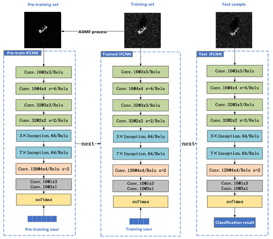
Figure 1.
The workflow and overall structure of the ADMF-IFCNN recognition method.
The workflow of the method includes three processes: pre-training, training, and testing. The ADMF method is utilized to generate pre-training samples, and it achieves better initialization of network parameters by completing network pre-training. Then the network is trained by training sets. The training set samples have not undergone any image processing operations, making it possible for the network to obtain all useful image information in training. Finally, testing the IFCNN.
On the overall structure of the method, one part is the ADMF process in Figure 1 corresponding to contribution 1 and contribution 3 described in Chapter 1. The ADMF is a processing method to reduce speckle noise, a pre-training set is constructed through the ADMF method, and it realizes network initialization through the pre-training process. The other part is the IFCNN network in Figure 1 corresponding to contribution 2 described in Chapter 1, the full convolution structure of the IFCNN can efficiently alleviate the overfitting problem. For small samples of SAR image recognition, the features extraction capacity is very critical of the network, therefore, the network introduces the Inception structure, the small-scale convolution kernel decomposition methods of the Inception structure increase the depth of the network, improve the generalization performance and the effective feature extraction capability. At last, the combination of mixed progressive convolution layers is applied to further reduce the computational burden of the network.
Next, we will introduce the ADMF method and the IFCNN model in turn.
2.2. Design of ADMF Method
Here, the ADMF method is a design based on the idea of an attention mechanism [30]. The essence of the attention mechanism is a series of attention distribution coefficients, that is, a series of weight parameters, which can be utilized to emphasize or select the important information of the processing object and suppress some irrelevant details. Our method and the method of attention mechanism are the same in thought, both of which are to strengthen the model’s attention and learning of target features, but the realization angle is different. The realization of the existing attention mechanism idea is mainly through giving the recognition network weight coefficient, hoping that the recognition network can notice the information that is more critical to the current task in a lot of information, and not pay too much attention to other non-critical information [31]. This paper proposes the ADMF method to realize the network’s focus on image targets from the perspective of network input, that is to say, we use the ADMF method to reduce noise interference, and use a small number of labeled samples to construct a large number of high-quality image samples for network parameter learning, which realizes more attention and learning for target from the network input.
The process of the ADMF method is shown in Figure 2. As shown in Figure 3a, the sample data of the original SAR image is recorded as a two-dimensional matrix A, and the mathematical expression of A is:
where i and j is the element in {1,2,…,128}, ai,j is the pixel value of the original image at the position (i,j).
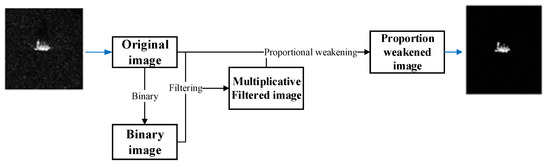
Figure 2.
Flow of ADMF image processing method.
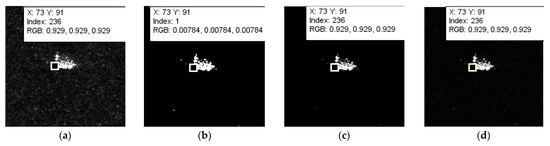
Figure 3.
Each stage of ADMF method: (a) original image; (b) binary image; (c) Multiplicative filtered image; and (d) proportion weakened image.
Set binarization threshold Bth, the original image A is binarized, and obtain a two-dimensional matrix X = [xi,j], it represents the binary image data, where xi,j is the pixel value of the binary image at the position (i,j) and the expression of xi,j is:
Then, the original image A and the binary image X are multiplied by the corresponding pixels to obtain the two-dimensional matrix Y = [yi,j], yi,j is the pixel value of the multiplicative filtered image at the position (i,j), and the expression of yi,j is:
Finally, the data information distribution ratio of the original image A and the multiplicative filtered image Y is 1:c, c is the representative of a series of parameters. According to the experimental feedback, i.e., network selection, a better c can be obtained, and the matrix Z:
where matrix Z is the two-dimensional data representation of the proportion-weakened image, zi,j is the pixel value of the proportion weakened image at the position (i,j). The last step of image processing is to allocate weight coefficients to the background and target in the image. For SAR image recognition, the network should focus on the extraction of target features. Therefore, by allocating a low weight coefficient of to the background information of the image, the background is weakened, and the network’s attention to the target from the perspective of the image is realized. In terms of image processing, the ADMF method is to process from the image amplitude domain, without changing the position information of the image, to achieve the enhancement of the target amplitude or the weakening of the background amplitude and so on.
Taking the SAR image target D7 as an example. By comparing Figure 3a,d, the ADMF method reduces speckle noise in the image without changing the target information. The binary processing of this method provides the possibility of image multiplicative filtering, as shown in Figure 3b, the process of binarization successfully retains the target area. It can be seen that the method can control the noise reduction amplitude of the image by setting the binary threshold and the weakening proportion coefficient. As shown in Figure 3c, the multiplicative filtered image represents the processing result when the weakening proportion is 0:1. The final image processing operation of this method is to achieve the purpose of constructing a large number of SAR image samples by setting the different weakening proportion coefficients, Figure 3d is the processing result when the weakening proportion is 1:10. From the perspective of attention mechanism, the learning of network parameters pays more attention to target characteristics, that is to utilize the ADMF method to construct a large number of target information prominent samples for network pretraining in this paper.
The ADMF method not only improves the quality of image samples but also achieves data augmentation. In addition, because the ADMF method is mainly aimed at image amplitude domain processing, the speckle noise in the radar imaging process covers a wide range in the frequency domain but is generally within a small range in the amplitude domain. At the same time, the location information of the image will not be changed through the ADMF method. So the ADMF method proposed in this paper is very practical in small sample SAR image target detection and recognition.
2.3. Design of IFCNN Model
We construct the IFCNN model by introducing the Inception structure and a combination of mixed progressive convolution layers into the FCNN, the structure of the IFCNN is shown in Figure 4.
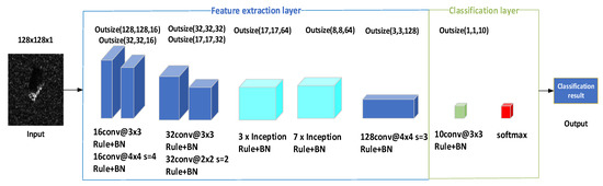
Figure 4.
The structure of IFCNN in this paper.
As shown in Figure 4, in the feature extraction layer of the IFCNN, the first two groups of convolution layers form a mixed progressive convolution layer structure through the exquisite stride and convolution kernel size design; the third group is the Inception structure, which contains 3 × Inception and 7 × Inception. The last layer is designed to implement the classification layer of the docking network. In addition, the Relu function and batch normalization are utilized.
The advantage of the IFCNN model is that it uses the basic framework of FCNN. With the help of the full convolution structure, we ingeniously designed a combination of mixed progressive convolution layers, which reduced redundancy calculations on the premise of weakening the influence of the large step on the network recognition accuracy. Then the Inception structure is easily introduced and improved. The Inception structure improves the depth of network feature extraction and accelerates the rate of network feature extraction through its dense computing mode. The introduction of the mixed progressive convolution layers and the Inception structure improve model feature extraction ability and training convergence performance better.
2.4. The FCNN and Mixed Progressive Convolution Layers
FCNN is a full convolution neural network, convolution structure can reduce the number of network parameters and alleviate the problem of network overfitting. The convolution layer in FCNN mainly convolutes the feature map of the upper layer with the learnable convolution kernel and then obtains the output feature map through an activation function. Each output characteristic graph can be combined to convolute the values of multiple characteristic graphs [32]:
where is the output of the jth channel of the convolution layer . For an output characteristic graph , the convolution kernel of each input characteristic graph may be different, is called the net activation, which outputs the characteristic graph to the upper layer is obtained after convolution sum and offset. Nj is utilized to calculate subset of input characteristics, is a convolution kernel matrix, is the offset of the convoluted characteristic graph. f( ) is the ReLU function.
In addition, compared with the pooling layer of traditional CNN, the convolution kernel can extract data features more effectively. As shown in Figure 5, two-dimensional data have the same data scale after passing through the convolution kernel and pooling layer, respectively, but the data generated by the convolution kernel is more relevant to the original two-dimensional data.
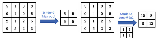
Figure 5.
Comparison between pooling layer and convolution layer.
Based on input and output characteristic mode of the convolution layer in FCNN and the advantages of using the convolution layer instead of the pooling layer, we design the mixed progressive convolution layers in FCNN. The large step of the convolution kernel can reduce the computational frequency and increase the network computing speed. However, if the large step is utilized continuously, some features will be lost and the recognition accuracy will be affected. However, the mixed progressive method can reduce the influence of the large step on the network recognition accuracy [28]. So we design the mixed progressive convolution layer structure, as shown in Figure 6.
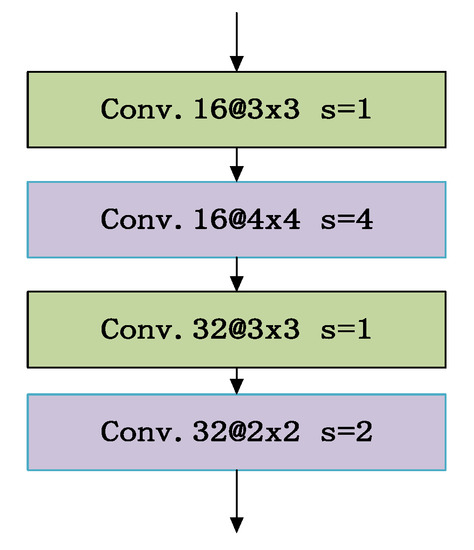
Figure 6.
The mixed progressive convolution layers.
The mixed progressive convolution layers are composed of a stride of 4 and size of 4 × 4 convolution kernel and a stride of 2 and size of 2 × 2 convolution kernel together with stride of 1 and size of 3 × 3 convolution kernels. The design of mixed progressive convolution layers in FCNN can save training time and the combination of convolution kernels with different sizes can increase the diversity of feature extraction.
2.5. The Inception Structure
The Inception structure is the multi-layer perceptron convolution layer. The multi-layer perceptron convolution layer utilizes the multi-layer perceptron model as a micro neural network, which is a generalized linear structure composed of a large number of filters, different from the conventional convolution layer by linear filters and nonlinear activation functions. The multi-layer perceptual convolution structure converts the full connection into a sparse connection, and clusters the sparse matrix into a relatively dense sub matrix, it can not only maintain the sparse characteristics of the filter level but also make full utilization of the high computing performance of the dense matrix [33]. The characteristic map is obtained by sliding in the input image. The calculation formula of it:
where, xi,j represents the image block to be processed when the convolution window is moved to the position (i,j), represents the connection weight between the convolution unit and input characteristic graph, the index of the feature graph needs to be extracted, is the offset value of the convolution unit.
In the Inception structure, a large number of 1 × 1 convolutional kernels are utilized to reduce the dimension of the data, introduce more nonlinearity, and improve the generalization ability [34]. In addition, considering that the convolution decomposition of the Inception structure cannot achieve a good effect in the early stage of the network model, it is usually utilized in the middle stage of the network, and the size of the feature map is about 12 to 20 [35]. Therefore, through calculation, the two Inception structures are set at the fifth and sixth layers of network feature extraction respectively, as shown in Figure 7.
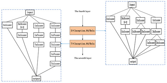
Figure 7.
The fifth and sixth layers of network feature extraction.
The two Inception structures are composed of 1 × 1, 1 × 3, 3 × 1, 1 × 7, and 7 × 1 convolution kernels in the form of unit blocks. The network performs joint filtering on the convolution results of convolution kernels of different sizes. The literature [36] verifies that these small-scale convolution kernel decomposition methods not only accelerate the convergence speed of the network but also increase the depth of the network and enhance the nonlinearity of the network. In this paper, the two Inception structures are improved, and the convolution kernel of a stride of 2 with a size of 3 × 3 is utilized to replace the pool to improve the model.
3. Experiments
3.1. Experimental Models and Datasets
To verify the effectiveness of the method proposed, we construct these models as follows.
The experimental networks include CNN, the FCNN, the IFCNN, the IFCNN 1, and the IFCNN 2. See Figure 8a for the CNN structure, Figure 8b for the FCNN structure, Figure 4 for the IFCNN structure, Figure 8c for the IFCNN1 structure, and Figure 8d for the IFCNN 2 structure.
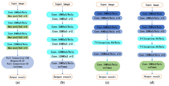
Figure 8.
Network structure: (a) CNN; (b) IFCNN; (c) IFCNN1; (d) IFCNN2.
In order to verify the performance of the proposed method, the Moving and Stationary Target Acquisition and Recognition (MSTAR) dataset is utilized for experiments. Select the ten-target samples at 15° and 17° depression angles from the MSTAR dataset. The 10 classes of targets on the MSTAR dataset are BMP2, BRDM2, 2S1, BTR60, BTR70, D7, T62, T72, ZIL131, and ZSU234. The samples at a depression angle of 17° are utilized for training, and the samples at a depression angle of 15° are utilized for testing.
To study SAR image recognition in the small sample, we build the experiment dataset. The subset-20 training dataset is established by randomly extracting 20 samples from targets of each category from the MSTAR dataset. Based on these 200 labeled training samples, we construct pre-training samples. First, we need to determine the range of parameters in ADMF, then expand data samples by setting parameters and finally label new data samples for network pre-training. The weakening proportion coefficient of the ADMF method is a flexible parameter, and its flexibility is reflected in the different ranges of the weakening proportion coefficient for different types of image recognition. In this paper, aiming at SAR image recognition, we have conducted exploratory experiments on the weakening proportion coefficient range. In Section 2.2, the c in the weakening proportion coefficient is a natural number. The subset-20 training dataset is processed once on each weakening proportion coefficient by ADMF method, and each c value corresponds to 20 × 10 samples. The CNN model in Figure 8 is trained to near convergence by the 200 samples. The results are shown in Figure 9.
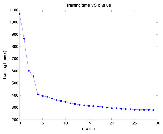
Figure 9.
Result of exploratory experiments on the weakening fusion ratio.
We find that the training time of the network changes greatly when c is less than 4. When c is greater than or equal to 4, the training time decreases slowly as c continues to increase. In addition, to consider reducing the occurrence of overfitting as much as possible, we preliminarily chose the weakening fusion ratio: 1:5, 1:10, 1:15, 1:20, and 1:25. Then 10 samples in targets of each category from the subset-20 training set are randomly extracted for ADMF image batch processing to obtain the subset-50 pretraining dataset, as shown in Figure 10.
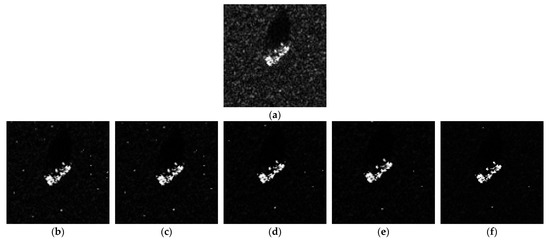
Figure 10.
Weaken fusion result (a) BTR60 original; (b) the fusion ratio is 1:5; (c) the fusion ratio is 1:10; (d) the fusion ratio is 1:15; (e) the fusion ratio is 1:20; (f) the fusion ratio is 1:25.
The testing dataset is created by selecting a sample from the MSTAR dataset. The pre-training samples, the training samples, and the testing sample are listed in Table 1.

Table 1.
The samples dataset of the experiment.
3.2. Experimental Results and Analysis
3.2.1. Experimental Simulation of ADMF Method
Here we carry out a four-target classification comparative experiment to verify the optimization effect of network initial parameters based on the ADMF image processing method. The network is supervised by the classification label, including the pre-training label and training label. In the Cuda10-Cudnn10.0-TensorflowGpu2.0 development environment, the random gradient descent algorithm is utilized to optimize the minimum loss function, the momentum is set to 0.95, the learning rate is set to 0.01, and the weight attenuation coefficient is set to 0.1.
The experiment steps are as follows:
- Configure the experiment environment and build the CNN, FCNN, and IFCNN. The convolution kernel weights of three networks are initialized by a normal distribution with a mean value of 0 and a standard deviation of , where n denotes the number of inputs to each unit [37];
- Then train three networks by the SAR subset-20 (see 0 for details). When the accuracy and loss of the training no longer change, adjust the learning rate by 10% until the learning rate reaches 10−7. Finally test and verify the three models and record the experimental results (the test sample targets are BMP2, T62, 2S1, and D7);
- Utilize the ADMF image processing method to structure the pre-training set, subset-50 (see 0 for details), after the pre-training of the network reaches convergence, and then repeat step 2;
Table 2.
Experimental results of four types of target classification.
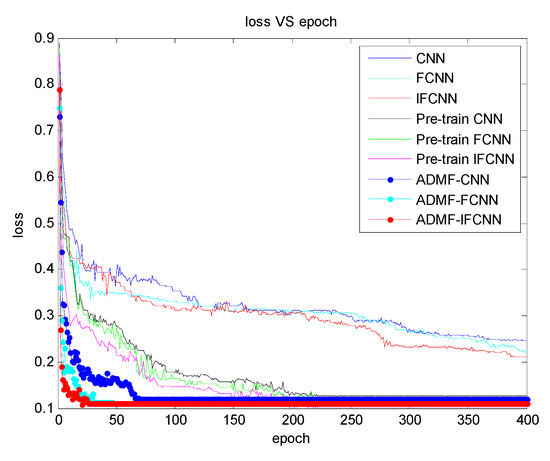
Figure 11.
Training loss curves of classification models.
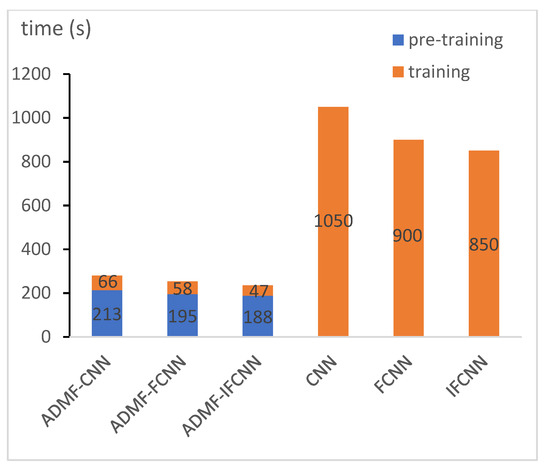
Figure 12.
The total time consumption of the pre-training and training process.
Table 2 shows the target recognition accuracy and training convergence time of the three networks through the process of pre-training and no pre-training. Figure 11 records each training convergence process of the three networks, namely the direct training process, pre-training process, and network training process after pre-training of CNN, FCNN, and IFCNN. Figure 12 shows the network time characteristic of each training convergence process.
From Table 2, we can see the testing accuracy and the average testing accuracy of the four-target. By comparing, the test accuracies of the three networks have been improved after the pre-training process, from the average testing accuracy data, the difference between the network pre-training and no pre-training results is close to 15%. In addition, the training convergence time of every network through pre-training has been greatly reduced; as shown in Figure 11, all three networks after pre-training reach convergence in about 60 epochs during the training process, while all three networks converge in about 210 epochs during the pre-training process. At last, all three networks still do not converge stably in 400 epochs during the direct training, which verifies the effectiveness of the pr-training method proposed.
In order to directly analyze the effectiveness of the pre-training method based on the ADMF proposed, we carry out time consumption statistics of the pre-training and training process, as shown in Figure 12. The data in Figure 12 shows the convergence time consumption of the pre-training and training process more intuitively. Compared with the network direct training method, the method adopting pre-training to improve the starting point of network training greatly saves time, although there is a network pre-training process, the overall training time does not increase but decreases significantly.
3.2.2. Comparative Experiments of IFCNN
Here we carry out the comparative experiment to study the recognition performance of the IFCNN model proposed. The model running environment and the experimental procedure are the same as in Section 3.2.1, and the testing accuracy of each type is listed in the last column of Table 3, Table 4 and Table 5. Since the convergence of various networks without a pre-training process is difficult under the condition of small samples, this comparative experiment is conducted on the basis of network pretraining.
Table 3.
Confusion matrix of testing results of the ADMF-IFCNN model trained on subset-20.
Table 4.
Confusion matrix of testing results of the ADMF-FCNN model trained on subset-20.
Table 5.
Confusion matrix of testing results of the ADMF-CNN model trained on subset-20.
The data in Table 3, Table 4 and Table 5 record the testing accuracy of ADMF-IFCNN, ADMF-FCNN, and ADMF-CNN for ten-target classification. Obviously, the testing accuracy of each target has been improved under the IFCNN model, including the average testing accuracy. In addition, the comparison between Table 3 and Table 4 shows that the average recognition accuracy of the ADMF-IFCNN model is 3.35% higher than that of ADMF-FCNN.
To more intuitively explore the reasons for the improvement of ADMF-IFCNN recognition performance compared with the other two models, we consider the differences in the output feature map size of each feature extraction layer, visualize the output feature map before classification and make a corresponding analysis [17]. As shown in Figure 13, Figure 13a is the input image (type of target ZIL131) for testing, and Figure 13b, Figure 13c, and Figure 13d show feature maps of a test image extracted by the trained ADMF-CNN, ADMF-FCNN, and ADMF-IFCNN, respectively.
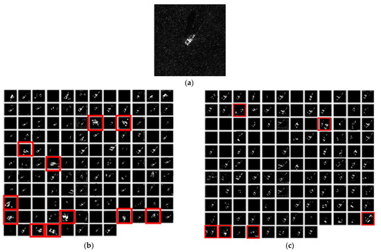
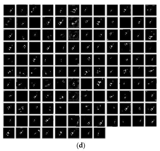
Figure 13.
Feature map output: (a) original image; (b) ADMF-CNN; (c) ADMF-FCNN; (d) ADMF-IFCNN.
As shown in Figure 13, the numbers of effective feature maps extracted by ADMF-IFCNN, ADMF-FCNN, and ADMF-CNN are 116, 99, and 106, respectively, the number of feature maps extracted by ADMF-IFCNN is more, it preliminarily shows that ADMF-IFCNN has stronger recognition ability. In addition, comparing Figure 13b–d, it can be seen that the feature map extracted by ADMF-IFCNN is sparser than ADMF-CNN and ADMF-FCNN. For example, the red mark in Figure 13b,c show that the sparsity of the feature map is poor, and the sparsity of the ADMF-CNN feature map is worse than the ADMF-FCNN. Sparse feature representations can effectively improve the generalization performance of the network [17,38] and good generalization of the network is conducive to improving the classification performance. ADMF-FCNN utilizes a full convolution structure to alleviate network overfitting and enhance the sparsity of the network [39], the results also show that the FCNN recognition accuracy is higher than that of ADMF-CNN; compared with ADMF-FCNN, ADMF-IFCNN introduces the Inception structure to the feature extraction layer. Theoretically, the joint filtering and the small-scale convolution kernel decomposition of the Inception structure have the ability to enhance the sparsity, so ADMF-IFCNN sparsity is further enhanced and network generalization is also enhanced, consistent with the experimental results.
The reason for the improvement of ADMF-IFCNN recognition performance is well explained by comparing the visualization results of feature maps and theoretical analysis, which also proves the effectiveness of the Inception structure we introduced.
3.2.3. Ablation Experiment of IFCNN
In order to further explore the influence of Inception structure and a combination of mixed progressive convolution layers on the performance of the network, two micro variable networks of IFCNN were constructed for this ablation experiment. As shown in Figure 8c, IFCNN1 removes 3×Inception (see Figure 7) from the feature extraction layer of IFCNN; as shown in Figure 8d, IFCNN2 is a micro variable network that changes the combination of mixed progressive convolution layers into conventional convolution layers of IFCNN. Then this paper compares each network’s training loss and testing accuracy on the subset-20, every network has gone through the pre-training process and completes the initialization of network parameters.
Figure 14 shows the convergence curves of five networks, of which Figure 14a is the convergence curve when the loss of the training set increases with the number of the epoch, and Figure 14b is the convergence curve when the classification accuracy of the test set increases with the number of the epoch. From Figure 14a, it can be seen that ADMF-IFCNN converges first, ADMF-IFCNN2 and ADMF-IFCNN1 converge successively, and finally, ADMF-CNN and ADMF-FCNN gradually converge. Comparing the training set loss convergence curves of ADMF-IFCNN and ADMF-IFCNN2 shows that the mixed progressive convolution layers can accelerate the convergence rate of network training. In Figure 14b, ADMF-IFCNN has the highest testing accuracy after convergence, testing accuracy of ADMF-IFCNN1 reveals a certain reduction compared to ADMF-IFCNN. Through comprehensive observation and analysis for Figure 14a,b, both the training convergence rate and testing accuracy of ADMF-IFCNN are higher than ADMF-IFCNN1, which effectively shows that the Inception structure can not only improve the network training convergence rate but also improve the network testing accuracy.
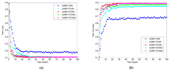
Figure 14.
Convergence curves of five network comparison algorithms (a) training set loss; (b) test set accuracy.
4. Discussion
At present, the experimental simulation results verify that the optimization method of network initial parameters is effective by pre-training based on the ADMF image processing method, but our exploratory experimental results also imply that it is easy to aggravate the network overfitting if we expand a large number of samples only by weakening the scale coefficient. To increase sample diversity to reduce the risk of overfitting caused by data augmentation, we adjust Formula (5) and add three parameters: n, m, and w to increase the diversity of pre-training samples, the parameter values are selected according to the purpose of image processing and exploratory experiment feedback.
As shown in Figure 15, Figure 15d is the result of target enhancement (parameter n is greater than parameter w) and Figure 15c is the result of target reduction samples (parameter n is less than parameter w). The research of target segmentation and target shadow region is of great significance for SAR recognition, so we also study target segmentation and target shadow region location through the ADMF method, the black area in Figure 15e is the target part and the black concentrated area in Figure 15f is the target shadow part. Target shadow region segmentation is still under study.
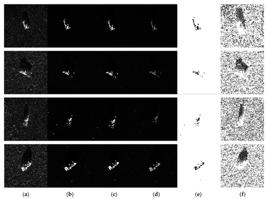
Figure 15.
Four class samples: (a) original image; (b) the fusion ratio is 1:10; (c) target enhancement; (d) target reduction; (e) target segmentation; (f) target shadow region location.
In addition, the ADMF method has been applied to the SSDD dataset, and it can also reduce speckle noise well, as shown in Figure 16. Figure 16b is the result of ADMF image processing when the weakening proportion coefficient is 1:10. Next, we will continue to study the improvement of the ADMF method and apply it to target detection and recognition in small sample SAR images.
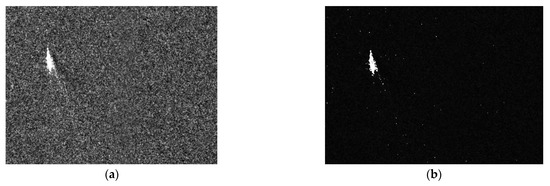
Figure 16.
SSDD data sample: (a) original ship image; (b) result of ADMF method.
This paper verifies that the ADMF-IFCNN model has better performance than ADMF-FCNN and ADMF-CNN in a small sample. To further demonstrate the advancement and superiority of our proposed method under limited SAR data, we compared the proposed recognition method with the existing recognition method, as shown in Table 6.
Table 6.
Comparison with the latest SAR recognition methods on MSTAR data subsets.
It should be emphasized that the test results of all methods in Table 6 are for ten types of target classification and the data sample in reference [40] and reference [17] is 88 × 88 patches from the original 128 × 128 SAR image chips. We can see that our proposed network achieves the best classification performance in all the comparison methods and the training convergence time is also the shortest. It is noteworthy that our ADMF-IFCNN method is less than 1% more accurate than the method in reference [25], but our training sample size is less. What is more noteworthy is that the attribute-guided multi-scale prototypical network (AG-MsPN) proposed in the literature [1] can achieve 92.68% recognition accuracy for 200 training samples, and their method can also achieve a better recognition rate for fewer samples. Our method has not achieved their effect in recognition accuracy, but their method is highly dependent on the prior information and the method implementation process is very complex. An extra attribute classification module (ACM) needs to be constructed based on prior knowledge and then used to complete the end-to-end training process with the MsPN, the training process also needs the joint supervision of the one-pot class label information from a few labeled data and the attribute information from the prior knowledge. Their method does not consider the time loss of end-to-end training and the subsequent impact when prior information is biased. For example, the results of subsequent studies may be biased, if the prior information is slightly biased in the design of ACM. So their methods are greatly affected by the prior information. However, the method proposed in this paper uses image data directly from model pre-training to training and does not need to construct abstract ACM to complete model training. Even if the pre-training sample label is wrong, the model will not continue to learn error information during training. In addition, we also optimize the training convergence performance, and our recognition model IFCNN still has room for improvement. The current research on the Inception structure is continuing, we also consider increasing the number of Inception appropriately or improving the Inception structure to improve the recognition capability of IFCNN for fewer samples.
5. Conclusions
In this paper, we propose a small sample SAR image target recognition method based on IFCNN combined with ADMF image processing. In Section 2, we introduce the design of the ADMF method and the IFCNN model. This paper builds IFCNN by introducing the Inception structure and a combination of mixed progressive convolution layers into the FCNN. The full convolution structure of FCNN effectively alleviates the problem of overfitting in limited data scenarios and improves the ability of feature extraction. In addition, a mixed progressive convolution layer on FCNN can not only achieve the effect of the pooling layer but also further accelerate the speed of network feature extraction by mixed strides. The Inception structure utilizes dense computing methods to realize accelerated training, which avoids the redundant computation of feature extraction to the greatest extent and enhances feature sparsity through small-scale convolution kernel decomposition and joint filtering. Based on the MSTAR dataset, the target classification experiment under a small sample scenario is carried out in Chapter 0. The results show that the recognition performance of the network is improved through pretraining. At the same time, through the comparative experiments of the three models, it is verified that the recognition performance of IFCNN is better, and the advantages of Inception structure and mixed progressive convolution layers for recognition are explained. In the discussion in Chapter 0, we further demonstrate the advancement and superiority of our proposed method by comparing it with the existing recognition methods. Our proposed method achieves higher testing accuracy and a faster training convergence rate with a simpler structure than other small sample recognition methods through comparison.
Finally, it is worth emphasizing that the ADMF method proposed in this paper provides a novel idea for data augmentation and target segmentation. This method utilizes the amplitude difference between the target and the background to reduce noise and improve the image quality, which is conducive to the research of small sample SAR image detection and recognition without changing the target position information of the image. In addition, the method is simple to implement and easy to improve, so it has very high practical value and research significance.
Author Contributions
Conceptualization, X.F.; Investigation, H.C. and J.D.; Methodology, H.C. and J.D.; Project administration, X.F.; Resources, X.F.; Validation, H.C.; Writing—original draft, H.C.; Writing—review and editing, H.C., J.D. and X.F. All authors have read and agreed to the published version of the manuscript.
Funding
This work was supported by 111 Project of China under Grant B14010. It is a funded project of China’s higher education.
Data Availability Statement
Not applicable.
Acknowledgments
The authors of this paper are grateful to the publishers of the MSTAR dataset, the authors of Inception-v4, and the editors and reviewers for their efforts and contributions.
Conflicts of Interest
The authors declare no conflict of interest.
References
- Wang, S.; Wang, Y.; Liu, H. Attribute-Guided Multi-Scale Prototypical Network for Few-Shot SAR Target Classification. IEEE J. Sel. Top. Appl. Earth Obs. Remote Sens. 2021, 14, 12224–12245. [Google Scholar] [CrossRef]
- Pei, J.; Huang, Y.; Huo, W.; Zhang, Y.; Yang, J.; Yeo, S.T. SAR Automatic Target Recognition Based on Multiview Deep Learning Framework. IEEE Trans. Geosci. Remote Sens. 2017, 56, 2196–2210. [Google Scholar] [CrossRef]
- Chen, S.; Wang, H.; Xu, F.; Jin, Y. Target Classification Using the Deep Convolutional Networks for SAR Images. IEEE Trans. Geosci. Remote Sens. 2016, 54, 4806–4817. [Google Scholar] [CrossRef]
- Wu, W.; Li, H.; Zhang, L.X. High-Resolution PolSAR Scene Classification With Pretrained Deep Convnets and Manifold Polarimetric Parameters. IEEE Trans. Geosci. Remote Sens. 2018, 56, 6159–6168. [Google Scholar] [CrossRef]
- Zeiler, M.D.; Fergus, R. Visualizing and Understanding Convolutional Networks. In Proceedings of the European Conference on Computer Vision (ECCV), Zurich, Switzerland, 6–12 September 2014; pp. 12–25. [Google Scholar]
- Houkseini, A.; Toumi, A. A Deep Learning for Target Recognition from SAR Images. In Proceedings of the Seminar on Detection Systems Architectures and Technologies, Algiers, Algeria, 20–22 February 2017; IEEE: Piscataway, NJ, USA, 2017; pp. 111–115. [Google Scholar]
- Amrani, M.; Jiang, F. Deep feature extraction and combination for synthetic aperture radar target classification. J. Appl. Remote Sens. 2017, 11, 1. [Google Scholar] [CrossRef]
- Du, Y.; Liu, J.; Song, W.; He, Q.; Huang, D. Ocean Eddy Recognition in SAR Images With Adaptive Weighted Feature Fusion. IEEE Access 2019, 7, 152023–152033. [Google Scholar] [CrossRef]
- Xiao, Z.; Liu, W. Research on SAR target recognition based on convolutional neural networks. Electron. Meas. Technol. 2018, 44, 15–27. [Google Scholar]
- Ding, J.; Chen, B.; Liu, H.W. Convolutional Neural Network With Data Augmentation for SAR Target Recognition. IEEE Geosci. Remote Sens. Lett. 2016, 13, 364–368. [Google Scholar] [CrossRef]
- Goodfellow, I.J.; Pouget-Abadie, J.; Mirza, M. Generative adversarial nets. In Proceedings of the 27th International Conference on Neural Information Processing Systems, Montreal, QC, Canada, 8–13 December 2014; pp. 2672–2680. [Google Scholar]
- Guo, J.Y.; Lei, B.; Ding, C.B. Synthetic Aperture Radar Image Synthesis by Using Generative Adversarial Nets. IEEE Geosci. Remote Sens. Lett. 2017, 14, 1111–1115. [Google Scholar] [CrossRef]
- Bao, X.J.; Pan, Z.X.; Liu, L. SAR Image Simulation by Generative Adversarial Networks. In Proceedings of the IGARSS 2019, Yokohama, Japan, 28 July–2 August 2019; pp. 9995–9998. [Google Scholar]
- Li, S.; Yue, X.; Shi, M. A Depth Neural Network SAR Occlusion Target Recognition Method. J. Xi’Univ. Electron. Sci. Technol. Nat. Sci. Ed. 2015, 31, 154–160. [Google Scholar]
- Huang, Z.; Pan, Z.; Lei, B. Transfer Learning with Deep Convolutional Neural Network for SAR Target Classification with Limited Labeled Data. Remote Sens. 2017, 9, 907. [Google Scholar] [CrossRef]
- Zhang, W.; Zhu, Y.; Fu, Q. Semi-Supervised Deep Transfer Learning-Based on Adversarial Feature Learning for Label Limited SAR Target Recognition. IEEE Access 2019, 7, 152412–152420. [Google Scholar] [CrossRef]
- Rui, Q.; Ping, L. A semi-greedy neural network CAE-HL-CNN for SAR target recognition with limited training data. Int. J. Remote Sens. 2020, 41, 7889–7911. [Google Scholar]
- Lingjuan, Y.; Ya, W. SAR ATR based on FCNN and ICAE. J. Radars 2018, 7, 136–139. [Google Scholar]
- Huang, Z.; Pan, Z.; Lei, B. What, Where, and How to Transfer in SAR Target Recognition Based on Deep CNNs. IEEE Trans. Geosci. Remote Sens. 2019, 58, 2324–2336. [Google Scholar] [CrossRef]
- Zhong, C.; Mu, X.; He, X. SAR Target Image Classification Based on Transfer Learning and Model Compression. IEEE Geosci. Remote Sens. Lett. 2019, 16, 412–416. [Google Scholar] [CrossRef]
- Wang, K.; Zhang, G.; Xu, Y. SAR Target Recognition Based on Probabilistic Meta-Learning. IEEE Geosci. Remote Sens. Lett. 2020, 18, 682–686. [Google Scholar] [CrossRef]
- Li, L.; Liu, J.; Su, L. A Novel Graph Metalearning Method for SAR Target Recognition. IEEE Geosci. Remote Sens. Lett. 2021, 19, 1–5. [Google Scholar] [CrossRef]
- Fu, K.; Zhang, T.; Zhang, Y. Few-shot SAR target classification via meta-learning. IEEE Trans. Geosci. Remote Sens. 2022, 60, 1–14. [Google Scholar]
- Zi, Y.; Fa, W. Self-attention multiscale feature fusion network for small sample SAR image recognition. Signal Process. 2020, 36, 1846–1858. [Google Scholar]
- Hang, W.; Xiao, C. SAR image recognition based on small sample learning. Comput. Sci. 2020, 47, 132–136. [Google Scholar]
- Pan, Z.X.; Bao, X.J.; Wang, B.W. Siamese Network Based Metric Learning for SAR Target Classification. In Proceedings of the IGARSS, Yokohama, Japan, 28 July–2 August 2019; pp. 1342–1345. [Google Scholar]
- Chen, Y.; Lingjuan, Y.U.; Xie, X. SAR Image Target Classification Based on All Convolutional Neural Network. Radar Sci. Technol. 2018, 1672–2337. [Google Scholar]
- Ling, L.; Qin, W. A SAR Target Classification Method Based on Fast Full Convolution Neural Network; CN111814608A; 2020; pp. 20–34.
- Chen, L.; Hong, W.U.; Cui, X. Convolution neural network SAR image target recognition based on transfer learning. Chin. Space Sci. Technol. 2018, 38, 45–51. [Google Scholar]
- Long, F.; Zheng, N. A Visual Computing Model Based on Attention Mechanism. J. Image Graph. 1998, 7, 62–65. [Google Scholar]
- Gao, K.; Yu, X.; Tan, X. Small sample classification for hyperspectral imagery using temporal convolution and attention mechanism. Remote Sens. Lett. 2021, 12, 510–519. [Google Scholar] [CrossRef]
- Bouvrie, J. Notes On Convolutional Neural Networks. In Tech Report; MIT CBCL: Cambridge, MA, USA, 2006; pp. 22–30. [Google Scholar]
- Lin, M.; Chen, Q.; Yan, S.C. Network in network. In Proceedings of the 2014 International Conference on Learning Representations, Banffff, AB, Canada, 14–16 April 2014; Computational and Biological Learning Society: Banffff, AB, Canada, 2014; pp. 24–37. [Google Scholar]
- Szegedy, C.; Vanhoucke, V.; Ioffe, S. Rethinking the Inception Architecture for Computer Vision. In IEEE Conference on Computer Vision and Pattern Recognition (CVPR); IEEE: Piscataway, NJ, USA, 2016; pp. 2818–2826. [Google Scholar]
- Szegedy, C.; Ioffe, S.; Vanhoucke, V. Inception-v4, Inception-ResNet and the Impact of Residual Connections on Learning. In Proceedings of the Thirty-First AAAI Conference on Artificial Intelligence, San Francisco, CA, USA, 4–9 February 2017; AAAI Press: Palo Alto, CA, USA, 2017; pp. 2913–2921. [Google Scholar]
- Min, X.; Hai, L.; Li, M. Research on fingerprint in vivo detection algorithm based on deep convolution neural network. Inf. Netw. Secur. 2018, 28–35. [Google Scholar]
- He, K.; Zhang, X.; Sen, S.; Sun, J. Delving deep into rectifiers: Surpassing human-level performance on imagenet classification. In Proceedings of the International Conference on Computer Vision, Las Condes, Chile, 11–18 December 2015; pp. 1026–1034. [Google Scholar]
- Barak, O.; Rigotti, M.; Fusi, S. The Sparseness of Mixed Selectivity Neurons Controls the Generalization-Discrimination Trade-Off. J. Neurosci. 2013, 33, 3844–3856. [Google Scholar] [CrossRef] [PubMed]
- Huesmann, K.; Rodriguez, L.G.; Linsen, L. The Impact of Activation Sparsity on Overfitting in Convolutional Neural Networks. In Lecture Notes in Computer Science; Springer: Berlin/Heidelberg, Germany, 2021; Volume 12663, pp. 130–145. [Google Scholar] [CrossRef]
- Ping, L.; Xiongjun, F.; Cheng, F.; Jian, D.; Rui, Q.; Marco, M. LW-CMDANet: A Novel Attention Network for SAR Automatic Target Recognition. IEEE J. Sel. Top. Appl. Earth Obs. Remote Sens. 2022, 15, 6615–6630. [Google Scholar]
- Chen, Y.; Wang, X.; Liu, Z.; Xu, H.; Darrell, T. A New Meta-Baseline for Few-Shot Learning. CoRR 2020, 6, 12–19. [Google Scholar]
- Sun, Y.; Wang, Y.; Liu, H.; Wang, N.; Wang, J. SAR Target Recognition With Limited Training Data Based on Angular Rotation Generative Network. IEEE Geosci. Remote Sens. Lett. 2019, 17, 1928–1932. [Google Scholar] [CrossRef]
Publisher’s Note: MDPI stays neutral with regard to jurisdictional claims in published maps and institutional affiliations. |
© 2022 by the authors. Licensee MDPI, Basel, Switzerland. This article is an open access article distributed under the terms and conditions of the Creative Commons Attribution (CC BY) license (https://creativecommons.org/licenses/by/4.0/).