Article

Dual-Constraint Registration LiDAR SLAM Based on Grid Maps Enhancement in Off-Road Environment

1
Hefei Institutes of Physical Science, Chinese Academy of Sciences, Hefei 230031, China
2
Science Island Branch, University of Science and Technology of China, Hefei 230026, China
*
Author to whom correspondence should be addressed.
Remote Sens. 2022, 14(22), 5705; https://doi.org/10.3390/rs14225705
Submission received: 9 October 2022 / Revised: 1 November 2022 / Accepted: 3 November 2022 / Published: 11 November 2022

Abstract

:
Aiming at the influence of fewer feature points and dynamic obstacles on location and mapping in off-road environments, we propose a dual-constraint LiDAR-based Simultaneous Localization and Mapping (SLAM) scheme. By abstracting LiDAR registration into two constraints, namely, in-window constraints and out-of-window constraints, the in-window constraints allow our scheme to compromise between accuracy and real-time performance, and out-of-window constraints can exploit optimized variables to provide richer constraint information. The advantages of incremental SLAM map construction can be used to design a variety of map forms. Although the variables outside the window are no longer involved in the optimization, we can use the two-dimensional probability grid map to provide binary semantic information and dynamic weights for the constraints outside the window to enhance the registration accuracy. Finally, we conducted experiments in off-road environment and compared with the mainstream LiDAR SLAM scheme, which can prove that our scheme has more advantages in accuracy.

1. Introduction

In the field of intelligent robots, localization and mapping are the basic modules for realizing autonomous capabilities. The localization module solves the problem of pose estimation and is indispensable in the robot’s obstacle avoidance and control. The mapping module mainly completes the environment modeling during the movement process, which is the prerequisite for decision making and path planning. With the development of the robotics field, intelligent robots are being increasingly used in off-road environments. However, it is usually difficult to carry out accurate positioning in the off-road environment because the intelligent robot is affected by factors such as unstructured roads and irregular environmental characteristics in the off-road environment. In terms of mapping, it is generally unnecessary to detect urban traffic elements such as lane lines and traffic lights in the off-road environment, but more attention is paid to the identification of the accessible area on the target task path (which can complete the global and local path planning). However, the road boundaries in the off-road environment are uneven, and sensors have blind sensing areas, which increases the difficulty of mapping. In practical applications, it is usually difficult to complete the environmental modeling of the off-road environment in advance, and the off-road environment is often an unknown environment. Simultaneous location and mapping (SLAM) can solve the problem of location and mapping simultaneously in unknown environments. The mainstream method is to use constraints to construct a nonlinear least squares problem and then solve it. Therefore, the constraint construction method and its weight calculation in the optimization function are key issues to consider.
LiDAR can perceive the obstacle information of the environment and output it in the form of point cloud data. Due to its high precision and strong anti-interference ability, it is widely used in the field of SLAM. In order to complete the autonomous navigation of the robot, a navigable grid map is essential. The grid map is scaled according to the scale of the real world, in which it is possible to mark whether the area is a passable attribute, which is one of the common output forms of SLAM.
According to the review by Cadena et al. [1], 1986 to 2004 was called the classical era of SLAM. During this period, some classical filtering-based SLAM methods were proposed, such as the method based on extended Kalman filters and Rao-Blackwellized particle filters. These methods and the maximum likelihood estimation method are no longer the mainstream methods due to the problems of excessive computation and memory consumption based on the filtering method in a large-scale environment. From 2004 to 2015 was called the era of algorithm analysis. It mainly analyzed the observability, convergence and consistency of SLAM. During this period, the concept of front-end and back-end was also proposed. The back-end is mainly used for optimization to minimize errors in the front-end, which mainly involves graph optimization, probability estimation, and numerical analysis.
The front-end registration methods of SLAM mainly include ICP [2] (Iterative Closest Point), NDT [3] (Normal Distributions Transform), optimization-based methods [4] and related matching methods CSM [5] (Correlative Scan Match). Among them, ICP contains a variety of variants, such as VICP [6], which can estimate the motion speed at the same time, and PL-ICP [7], which constructs a point-line metric ICP that is more in line with the real physical environment. Ji Zhang et al. [8] proposed a real-time LiDAR odometry and mapping method, LOAM, and it has been in a state-of-the-art position since it was proposed. Its advantage is that it extracts line and surface feature points and uses the optimization method based on point line and point surface for registration, which is essentially a variant of ICP. However, this method of extracting feature points significantly improves computing efficiency and stability. It can achieve very good registration effects in real time.
At present, the mainstream SLAM back-end method is based on graph optimization. Ref. [9] is the pioneering work of SLAM based on graph optimization and was first implemented by [10]. For graph-optimized SLAM using LiDAR as the main sensor, Tixiao Shan et al. proposed a smoothing and map-building, tightly coupled LiDAR-inertial odometry (LIO-SAM) [11], which implemented a graph-optimized framework based on iSAM2 [12] and added constraints such as inter-frame point cloud registration, IMU pre-integration, GPS and loop closure. Although the open source implementation adopts a direct truncation method for the fusion IMU pre-integration part, it has a good reference in the engineering sense. Haoyang Ye et al. proposed a tightly coupled LiDAR-inertial odometry and mapping (LIO-Mapping) [13] framework, which is used to maintain the scale of variables in graph optimization based on the sliding window method; the point-line of the feature point cloud between frames, point-surface registration constraints and constraints such as IMU pre-integration are jointly optimized. The sliding window algorithm removes some optimization variables so as to maintain the keyframes within a certain size; however, directly removing optimization variables affects the accuracy, so marginalization constraints are usually added [14]. Unlike LIO-SAM, LIO-Mapping adopts a marginalized method, which is more reasonable and complete on a theoretical basis. However, in practical application effects, LIO-Mapping takes each feature point as a constraint, and LIO-SAM has degenerated the constraints of multiple feature points into pose increment constraints. In addition, the amount of calculations in LIO-Mapping is much larger than that of LIO-SAM. However, in unknown and possibly loop-free environments, sliding-window-based optimization methods are more applicable. Kaijin Ji et al. proposed a SLAM algorithm based on a grid which combines probability and features by expectation maximization (EM) [15].
Intelligent robots need not only high-precision positioning, but also high-precision navigation maps when completing traffic mapping. The construction method of the classic two-dimensional probability grid map is mature, and the traditional two-dimensional LiDAR SLAM scheme uses the probability grid map as the output target, such as Gmapping [16], Cartographer [17] and so on. As early as 1989, Moeavec proposed a probability method for occupancy grid maps [18]. By assigning each grid an occupancy probability value, and using the LiDAR inversion observation model to dynamically update the occupancy probability, the two-dimensional probability grid can be obtained. The map distinguishes traversable areas and removes the effects of dynamic obstacles in multiple observations. The most advanced three-dimensional LiDAR SLAM algorithm LOAM [8] and a series of variant mapping algorithms (such as Lego LOAM [19]) are all discrete point cloud maps obtained by directly splicing point clouds, which can be used to create Octomap [20]. It is also easy to navigate when compressing maps, but due to the impact of dynamic obstacles, it will leave ghosts on the map. To remove dynamic obstacles, Xieyuanli Chen et al. proposed SuMa++ [21], which takes bins as map elements and then introduces the difference of semantic information as observation information to dynamically update the stability of the bins and directly eliminate unstable bins. However, maintaining bins requires a lot of resources.
For the demand of off-road environment map construction, we should give full play to the advantages of incremental SLAM map construction and design a variety of map forms, for example: using satellite maps to complete the global path planning of vehicles, using point cloud maps for location registration and using grid maps for local path planning. The construction of grid maps will be integrated based on filtering algorithms and have richer local perceptual information than single-frame data to narrow the perceptual blind area. The obstacle occupation information in the observation area can be updated many times to provide feedback information for vehicle positioning. As a common navigation map, a probability grid map is preferred. In an unstructured off-road environment, different observations may determine different traffic results for a region, such as the observation of steep slopes at different angles, the observation of dynamic obstacles, etc. Therefore, it is necessary to dynamically update the traffic probability by integrating multi-frame observation results. However, 3D probability grids are rarely used due to the problem of excessive computation, and other forms of 3D maps also require a lot of resources.
The current mainstream 3D LiDAR SLAM solution is to insert the scan-to-map constraint of the point cloud into the graph optimization framework, and this constraint can only constrain the current pose and cannot take advantage of the graph optimization. In order to take advantage of LiDAR constraints, this paper will generate the widely used LiDAR and occupancy grid map, propose a dual-constraint construction method using LiDAR and use the grid map as the medium to calculate the weight of the constraint. The main contributions of this paper are as follows:
  • For the SLAM algorithm based on sliding window optimization, two constraint construction methods for LiDAR are proposed—in-window constraints and out-of-window constraints—to make up for the disadvantage of having fewer feature points during the inter-frame registration in off-road open scenes. According to the size of the sliding window, the pose accuracy and algorithm solution time can be compromised;
  • Using the grid map as a medium, the occupancy information of the grid map is abstracted into the binary semantics of occupancy, weighting the out-of-window constraints of the LiDAR and further proposing a strategy based on a two-dimensional grid map to eliminate dynamic obstacles in the point cloud map.
The remainder of this paper is organized as follows. Section 2 describes the proposed method specifically. Then, Section 3 shows and analyzes the experiment results, Section 4 carries out relevant discussions and presents prospects for future work, and Section 5 summarizes the article.

2. Methods

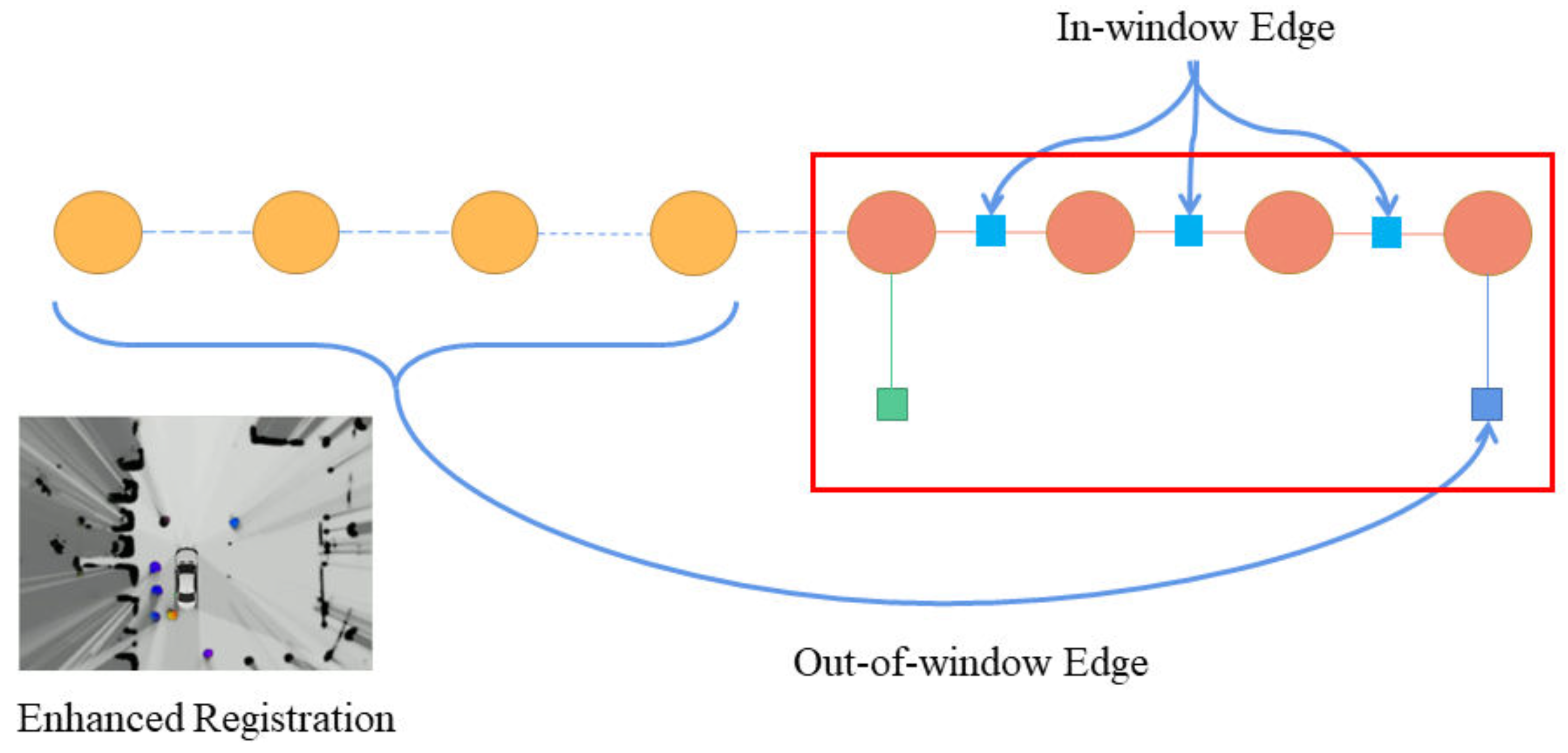
The system framework is shown in Figure 1. We use the graph optimization method based on a sliding window to build a SLAM system and abstract the constraints of LiDAR into two constraints, namely, the constraint edge inside the window and the constraint edge outside the window. The residual edge in the window is a binary edge, similar to ICP, by taking the distance value of the matching point as the error, and adjusting the two-frame pose associated with it. The residual outside the window is an unary edge, and the key frame outside the window is extracted to form a local map to match the point cloud of the current frame. Since the optimization variables outside the window will not be adjusted, only the pose of the current frame is adjusted. In order to provide better constraint information for the residual outside the window, we use a two-dimensional grid map. The grid map is used to dynamically adjust the weights of the constraint edges outside the window to enhance the point cloud registration.

2.1. Graph Optimization Based on a Sliding Window

In the graph optimization fusion framework, the “vertices” in the graph are used as optimization variables, which are usually the pose of the vehicle in the localization (the graph is also called a Pose Graph). The “edges” in the graph are used as constraints (that is, observation) and are divided into the unary edge, binary edge and multi-element edge according to the number of optimization variables bound by constraints. For example, the GPS absolute localization constraint is the unary edge, and IMU, wheel odometer, inter-frame registration, loopback and other constraints are binary edges. For example, the observation equation of the binary edge is: z = f ( X 1 , X 2 ) , where X i is the 6-DOF pose, and X = [ θ r o l l , θ p i t c h , θ y a w , x , y , z ] T . Considered from the perspective of least squares, the observed residuals can be written as: e ( X ) = z f ( X 1 , X 2 ) . If we add other observations, we can obtain the overall cost function:
F ( X ) = 1 2 i = 1 m | | e i ( X ) | | 2 = 1 2 i = 1 m | | z i f i ( X ) | | 2
where X = [ X 1 , X 2 , . . . , X n ] T , n represents the number of optimized poses.
The optimization equation is solved by the Gauss–Newton method, that is, each residual term is first-order expanded and then squared and summed. For example, the first-order Taylor expansion of the residual of the k observation is performed:
e k ( X + Δ X ) = e k ( X ) + J k Δ X
So, the nonlinear function can be approximated as:
F ( X + Δ X ) = k ( f k ( X ) T f k ( X ) + 2 f k ( X ) T J k Δ X + Δ X T J k T J k Δ X )
Differentiate Δ X and set the result to 0:
k J k T J k Δ X = k J k T f k ( X )
Therefore, the equations built each time look like this:
H Δ X = b
However, as time goes on, there will be more and more poses. In order to avoid excessive calculation in the optimization process, the sliding window method is used to control the scale of the optimization variables. When an optimization variable needs to be discarded, it should be considered that the information after the linearization of the variable in the last iteration of the variable remains in the H matrix and b vector, and this information should be transferred to the remaining variables. Therefore, it is necessary to compare the H matrix and b vector. The vector is marginalized, and the optimization variables that need to be discarded in Equation (6) are disassembled:
H r r H r m H m r H m m Δ X r Δ X m = b r b m
where Δ X r is the reserved optimization variable, and Δ X m is the optimization variable that needs to be marginalized, so the reserved variables are constrained by the following:
( H r r H r m H m m 1 H m r ) Δ X = b r H r m H m m 1 b m
Rewrite it as:
H p Δ X p = b p
This constraint is used as a prior constraint and directly added to the next iteration, but the prior constraint has lost the residual information. After the remaining variables are adjusted, it is necessary to dynamically adjust the right-hand side of Equation (8). The half side is updated, assuming that X p changes δ X p ; then, it is equivalent to δ X p changing δ X p . Then, the right half is updated as:
b p b p H p δ X p
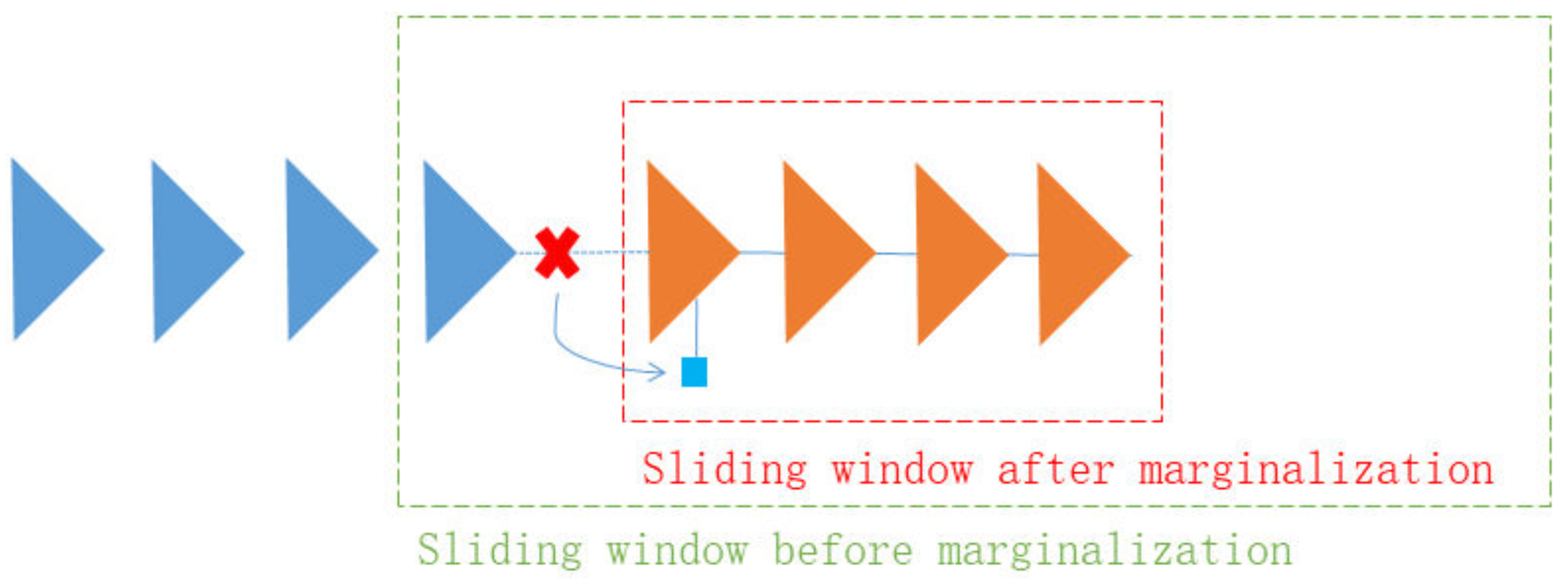
So far, the graph optimization solution framework based on a sliding window has been completed. The sliding window’s marginalization is shown in Figure 2. The process of marginalization is mainly described intuitively, that is, the constraint information of the variables to be discarded is transferred to the prior constraints of the variables in the window.

2.2. In-Window Constrains

For the in-window constraint of LiDAR, it is similar to the scan-to-scan registration of LiDAR, that is, the point–line and point–surface distances between frames are constructed as errors, where a “point” is the feature point of the current frame, and “line” and “surface” are the feature points of the previous frame. Thus, for each feature point, the registration error between frames can be obtained as:
e i = s i T ( T k k 1 p i L k p i L k 1 )
where s is the normal vector of the line and surface features, p i L k is the laser point of the k frame, p i L k 1 is the laser point that matches the p i L k of the k 1 frame and T k k 1 is the conversion of the laser point from the k frame to the k 1 frame transformation.
Since the optimization variable is the pose vector under the w system, it is necessary to transform T k k 1 in Equation (10):
T k k 1 = T k 1 w 1 T k w
Since Equation (11) is bound to two poses, and both poses need to be optimized, the constraint edge is a binary edge, which can be called the “in-window residual” of LiDAR. This constraint is added to the graph optimization solution framework, and the residuals and normals of the line and surface features, as well as the Jacobian matrix of the residuals to the optimization variables, need to be calculated.
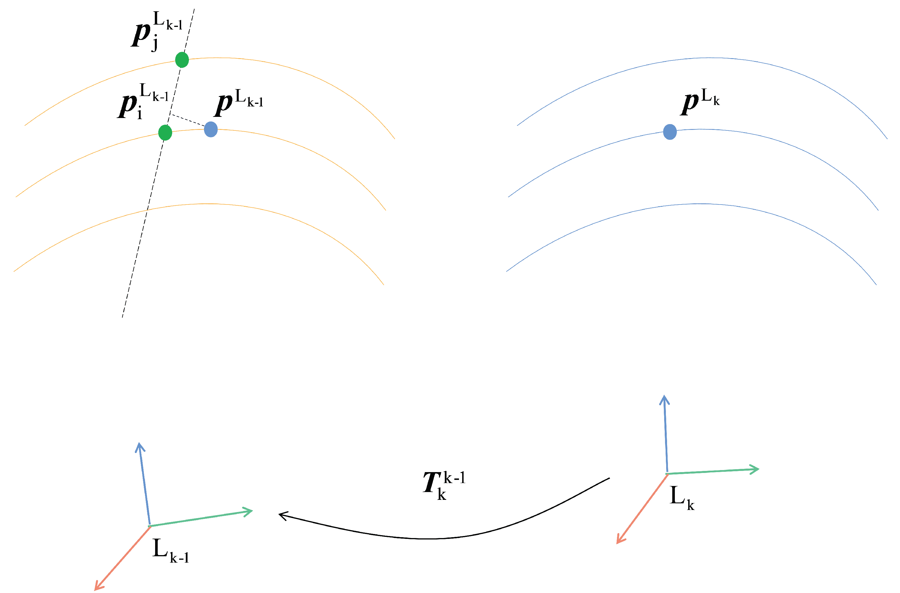
For line features, as shown in Figure 3, first transform the line feature point p L k of the k frame to p L k 1 in the k 1 frame according to the current pose estimation, and search for the nearest Euclidean distance to p L k 1 in the k 1 frame. The line feature point p i L k 1 is searched again for the nearest line feature point p i L k 1 in the adjacent LiDAR beams of the k 1 frame and p j L k 1 , thus avoiding the collinearity of the three points p L k 1 , p i L k 1 and p j L k 1 and taking the distance between p L k 1 and the straight line p i L k 1 p j L k 1 as the residual. The residual error is minimized by adjusting the poses of the k 1 frame and the k frame.
The residual and normal vector can be calculated by obtaining the three points p L k 1 , p i L k 1 and p j L k 1 . The residual and normal vector can be calculated by calculating the area of the parallelogram with the line segment p L k 1 p i L k 1 and the line segment p L k 1 p j L k 1 as the side lengths and the length of the line segment p i L k 1 p j L k 1 :
e = | ( p i L k 1 p L k 1 ) × ( p j L k 1 p L k 1 ) | | p i L k 1 p j L k 1 |
s = ( p i L k 1 p j L k 1 ) × ( ( p i L k 1 p L k 1 ) × ( p j L k 1 p L k 1 ) ) | ( p i L k 1 p j L k 1 ) × ( ( p i L k 1 p L k 1 ) × ( p j L k 1 p L k 1 ) ) |
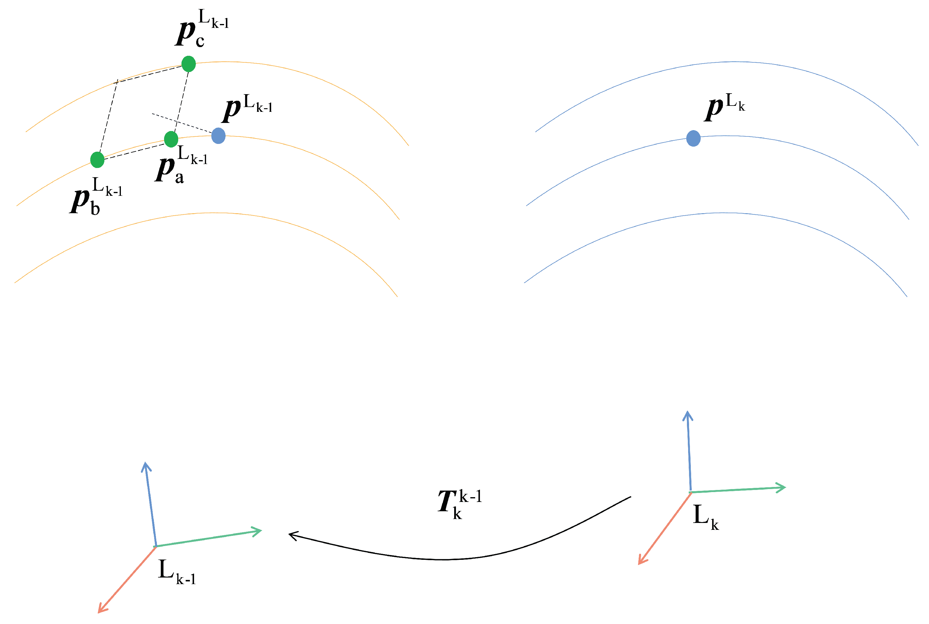
For the surface feature, as shown in Figure 4, first transform the surface feature point p L k of the k frame to p L k 1 in the k 1 frame according to the current pose estimation and search for the nearest Euclidean distance to p L k 1 in the k 1 frame. The surface feature point p a L k 1 of the k − 1 frame is searched again for the nearest surface feature point p b L k 1 in the same LiDAR beam as p a L k 1 and the nearest surface feature point p c L k 1 in the adjacent LiDAR beam with p a L k 1 , thus avoiding p L k 1 , p a L k 1 , p b L k 1 and p c L k 1 . The four points are coplanar; the distance between p L k 1 and the plane p a L k 1 p b L k 1 p c L k 1 is used as the residual; and the residual is minimized by adjusting the poses of the k 1 frame and the k frame.
The residual and normal vector can be calculated by obtaining the four points p L k 1 , p a L k 1 , p b L k 1 and p c L k 1 . The residual can be calculated by the area of the parallelogram with the line segments p b L k 1 and p c L k 1 as the side lengths and its normal vector:
s = ( p b L k 1 p a L k 1 ) × ( p c L k 1 p a L k 1 ) | ( p b L k 1 p a L k 1 ) × ( p c L k 1 p a L k 1 ) |
e = s T ( p L k 1 p a L k 1 )

2.3. Constrained Edge outside the Window

For the pose outside the sliding window, we can select the part that has a common viewing area with the current vehicle localization. Since the variables outside the window are no longer involved in the optimization, we can directly convert their point cloud data to the global coordinate system as a local map. Then, a registration constraint between the current frame and the local map is constructed, which is similar to the scan-to-scan registration of LiDAR and can make up for the defect of fewer feature points during inter-frame registration.
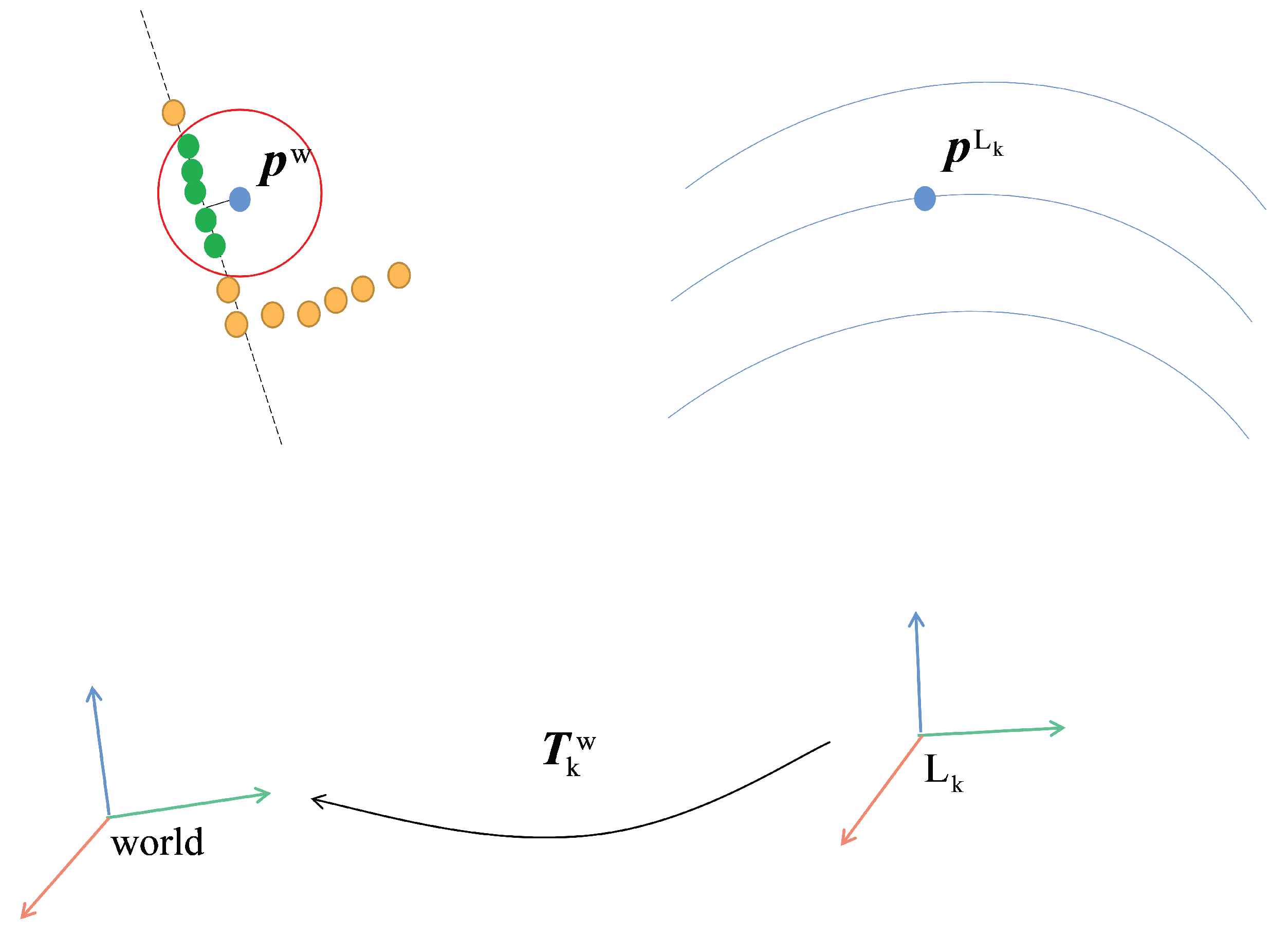
For line features, as shown in Figure 5, first transform the line feature point p L k of the k frame to p w in the world system according to the current pose estimation, and search for the 5 line feature points in the local map that are closest to the Euclidean distance of p w (that is, the green point in the Figure 5). Next, solve the mean and covariance matrix of these five points using Equations (16) and (17) and decompose the covariance matrix of Equation (17) by SVD, finally obtaining the minimum eigenvalue. The corresponding feature vector is the normal vector of the line feature. Through the mean value p c e n t e r w and normal vector of these 5 points, 2 virtual matching points, p i w and p j w , can be generated, corresponding to p i L k 1 and p j L k 1 in Figure 5. Then, directly use Equations (12) and (13) to solve residuals and normals for outgoing features:
p c e n t e r w = k = 1 5 p k w
= k = 1 5 ( p k w p c e n t e r w ) ( p k w p c e n t e r w ) T
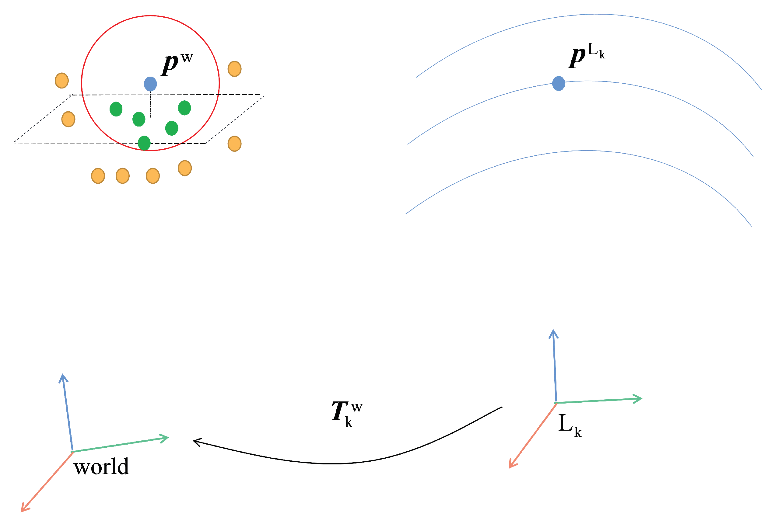
For surface features, as shown in Figure 6, first transform the surface feature point p L k of the k frame to p w in the world system according to the current pose estimation, and search for the five surface feature points in the local map that are closest to the Euclidean distance of p w (the green dots in the Figure 6) and the plane equation from them:
a x + b y + c z + 1 = 0
The parameters a, b and c in the plane equation in Equation (18) are formulated by linear least squares and solved by constructing Equation (19):
x 0 y 0 z 0 x 1 y 1 z 1 x 2 y 2 z 2 x 3 y 3 z 3 x 4 y 4 z 4 a b c = 1 1 1 1 1
After the plane equation is solved, the point-to-plane distance can be calculated by substituting p w into the following equation, which is directly used as the residual:
e = a x + b y + c z + 1 a 2 + b 2 + c 2
Among them, the plane normal vector that makes the absolute value of the residual along the increasing direction is:
s = [ a b c ] T

2.4. Occupancy Grid Map Construction Method

The impassable area is often a place with a steep slope. This article will mark the obstacle by calculating the slope of the laser point. If the slope is too large, it will be marked as an obstacle point, which can effectively segment the obstacle. The equation for calculating the slope of the laser point is:
θ = arctan ( z 1 z 2 ( x 1 x 2 ) 2 + ( y 1 y 2 ) 2 )
Among them, ( x 1 , y 1 , z 1 ) is the laser point for calculating the slope, and ( x 2 , y 2 , z 2 ) is the laser point in the adjacent row and the same column of the laser point on the range image. In this paper, the laser point whose slope exceeds the threshold is marked as an obstacle, indicating that the area is impassable. The schematic diagram is shown in Figure 7, where the part marked in red will be regarded as an obstacle point cloud. It can be seen in the figure that the single point cloud observation of the frame will have blind spots due to the angle problem, and it is necessary to integrate the information of multiple frames to construct an accurate navigation map.
Project the point cloud marked with slope obstacles to the two-dimensional elevation grid map and the occupancy grid map. Binary data are occupied by obstacles. When the point cloud is projected to the grid, if the laser point has been marked as an obstacle according to the slope, it is directly marked in the corresponding occupied grid, and the maximum height and minimum height projected to the corresponding elevation grid are recorded at the same time. When a grid is projected by the laser point, it can be called observable, and the height difference of all observable grids is calculated one by one. If the height difference is greater than the threshold, it will be marked in the occupied grid, as shown in Figure 8. A schematic diagram of the projection of a single point cloud frame to the occupancy grid map, that is, the grid with a large slope or a large height difference in the grid is marked as the occupied grid and represented by a red border.
This paper expresses the global occupancy grid map by introducing occupancy probability. Different from 2D LiDAR SLAM, this paper has already marked the grid with obstacles, so there is no need to use the hitting point or passing point of the laser beam to carry out update. In order to avoid the huge amount of calculation in the 3D scene, we use binary Bayesian filtering to update the occupancy probabilities. We assume that occupancy values between grids are independent and establish a posterior probability for each occupied grid m i :
p ( m i | x 1 : k , z 1 : k )
where x 1 : k and z 1 : k represent the pose and occupancy observations, respectively, from the first to the k frame (binary observations, that is, whether it is an obstacle or not); that is, infer the occupied grid from the pose and occupancy observations of all historical frames. For Equation (23), using the Bayesian formula, we can obtain:
p ( m i | x 1 : k , z 1 : k ) = p ( z k | m i , x 1 : k , z 1 : k 1 ) p ( m i | x 1 : k , z 1 : k 1 ) p ( z k | x 1 : k , z 1 : k 1 )
Since the observations are independent of each other and are only related to the pose and state at the current moment, and the grid state is simultaneously related to the pose and state at a certain moment, the above equation can be rewritten as:
p ( m i | x 1 : k , z 1 : k ) = p ( z k | m i , x k ) p ( m i | x 1 : k 1 , z 1 : k 1 ) p ( z k | x k )
Furthermore, using the Bayesian formula on the above equation, we obtain:
p ( m i | x 1 : k , z 1 : k ) = p ( m i | x k , z k ) p ( m i | x 1 : k 1 , z 1 : k 1 ) p ( m i | x k ) = p ( m i | x k , z k ) p ( m i | x 1 : k 1 , z 1 : k 1 ) p ( m i )
Then, the probability ratio is:
p ( m i | x 1 : k , z 1 : k ) p ( ¬ m i | x 1 : k , z 1 : k ) = p ( m i | x k , z k ) p ( m i | x 1 : k 1 , z 1 : k 1 ) p ( ¬ m i ) p ( m i ) p ( ¬ m i | x k , z k ) p ( ¬ m i | x 1 : k 1 , z 1 : k 1 )
Take the logarithm of both sides:
log p ( m i | x 1 : k , z 1 : k ) p ( ¬ m i | x 1 : k , z 1 : k ) = log p ( m i | x 1 : k 1 , z 1 : k 1 ) p ( ¬ m i | x 1 : k 1 , z 1 : k 1 ) + log p ( m i | x k , z k ) p ( ¬ m i | x k , z k ) log p ( m i ) p ( ¬ m i )
Define Log Odds Ratio to better describe:
l ( x ) = log p ( x ) 1 p ( x )
Then, Equation (28) can be rewritten as:
l ( m i | x 1 : k , z 1 : k ) = l ( m i | x 1 : k 1 , z 1 : k 1 ) + l ( m i | x k , z k ) l ( m i )
where l ( m i | x 1 : k , z 1 : k ) is the inferred grid occupancy probability logarithm from frames 1 to k, l ( m i | x 1 : k 1 , z 1 : k 1 ) is the inferred grid occupancy probability logarithm from frames 1 to k 1 , and l ( m i | x k , z k ) is the grid occupancy probability observed in the k frame The number of comparisons, l ( m i ) , is the number of the prior grid occupancy probability ratios.
When the grid is observed in a certain frame, the occupancy probability logarithm of the grid observed in this frame is added, and then converted to the occupancy probability by the following:
p ( x ) = 1 1 1 + exp ( l ( x ) )

2.5. Enhanced Registration

SLAM is simultaneous localization and mapping, in which Localization and Mapping are two independent modules, but they are simultaneously estimated. When all sensors are gathered for pose estimation, feeding back the constructed historical map to the localization module can not only further improve the localization accuracy, but also improve the consistency of the map because the current localization and environment observations are also inserted into the map for updates.
The feedback from the map to the localization module is the essence of SLAM. The common feedback method is to construct a local map to construct a scan-to-map constraint, that is, the constraint edge outside the window mentioned above. Although the variables outside the window cannot be optimized again, we constructed a grid map can also provide additional feedback information. The following mainly discusses the feedback method of the two-dimensional grid map.
The probability grid map actually gives semantic information to a certain extent, that is, the binary semantics of whether the area is an obstacle, so this information can be used to improve the accuracy of point cloud registration (enhanced registration). In the part of the constraint edge outside the window, this paper constructs the registration constraint of scan-to-map on the LiDAR constraint, in which the map part is constructed using the keyframes outside the sliding window. Since these frames are no longer involved in the optimization, the local maps constructed from keyframes are also not adjusted. Then, during scan-to-map registration, it is very reasonable to weight each feature point by drawing on the occupancy grid map of the current frame and the obstacle occupancy information of the global occupancy grid map. The weight of each constraint can be set as:
w i k = æ H u b e r ( e i k ) · C s e m a n t i c ( S i L k , S j w )
where æ H u b e r ( · ) is the Huber robust kernel function, whose definition is shown in Equation (33), and C s e m a n t i c ( S i L k , S j w ) is the semantic weight of the matching point between the current frame and the global map with binary semantic labels, whose definition is shown in Equation (34):
æ Huber ( e ) = 1 , if | e | < δ δ | e | 1 , otherwise
C semantic y i L k , P i L k , y j w , P j w = p y i L k i if y i L k = y j w 1 p y i L k i otherwise
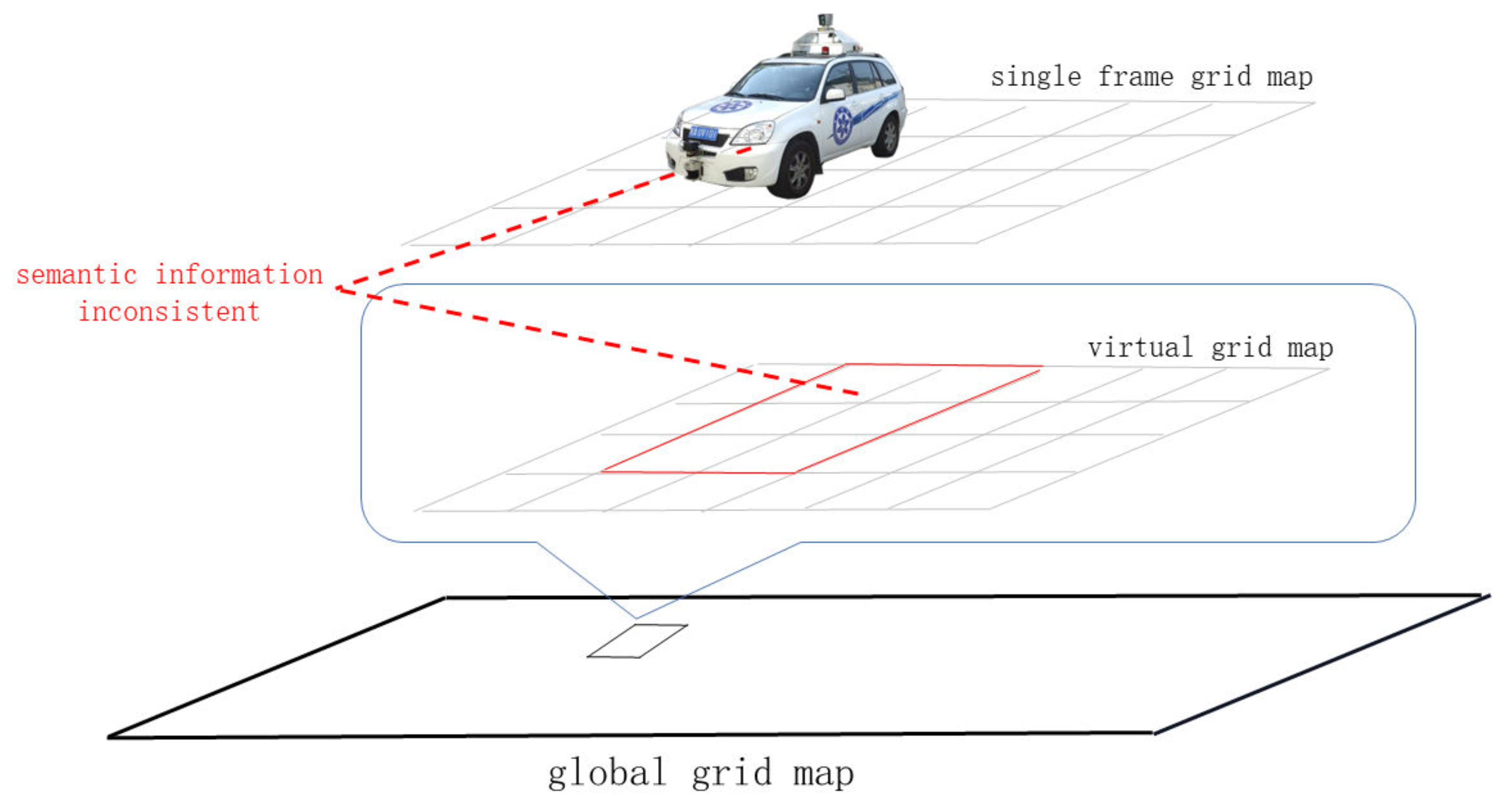
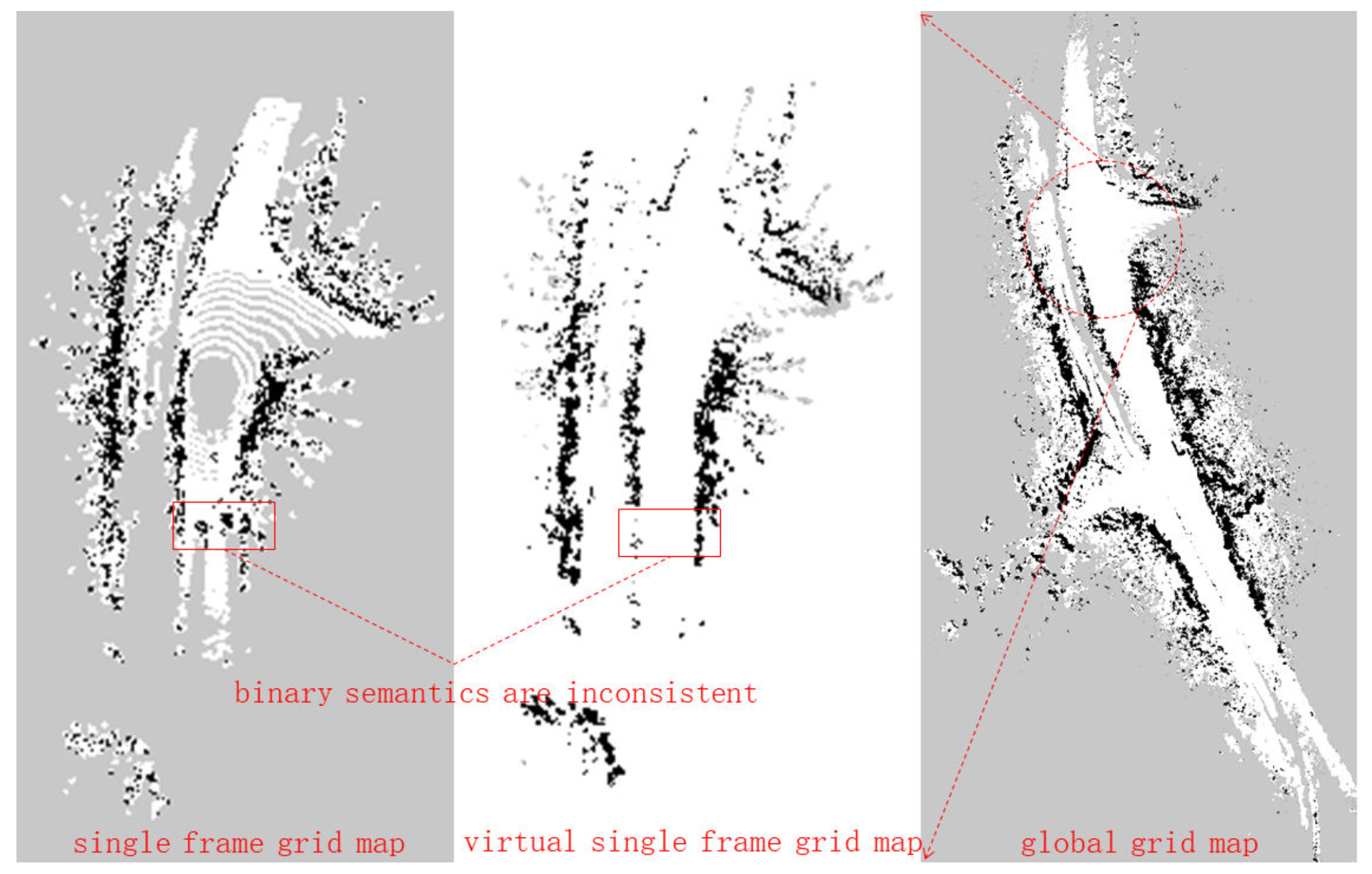
Among them, y i L k and y j w are the semantic labels of the current frame and the next pair of matching points in the global coordinate system. For matching points with consistent semantics, the weight of p y i L k i is given. In the program implementation, p y i L k i can be set according to the occupancy probability value. Figure 9 is the illustration of the enhanced registration. By generating a virtual single-frame occupied grid map from the global map, a binary semantic comparison is made with the occupied grid map of this frame. Because dynamic obstacles have less impact on the global grid map, the area where the dynamic obstacle is located is likely to be semantically inconsistent. According to Equation (34), the semantic weight of the laser point registration in this area will generate a very small value to reduce the registration process effects of small dynamic obstacles.
3. Results

3.1. Experimental Platform

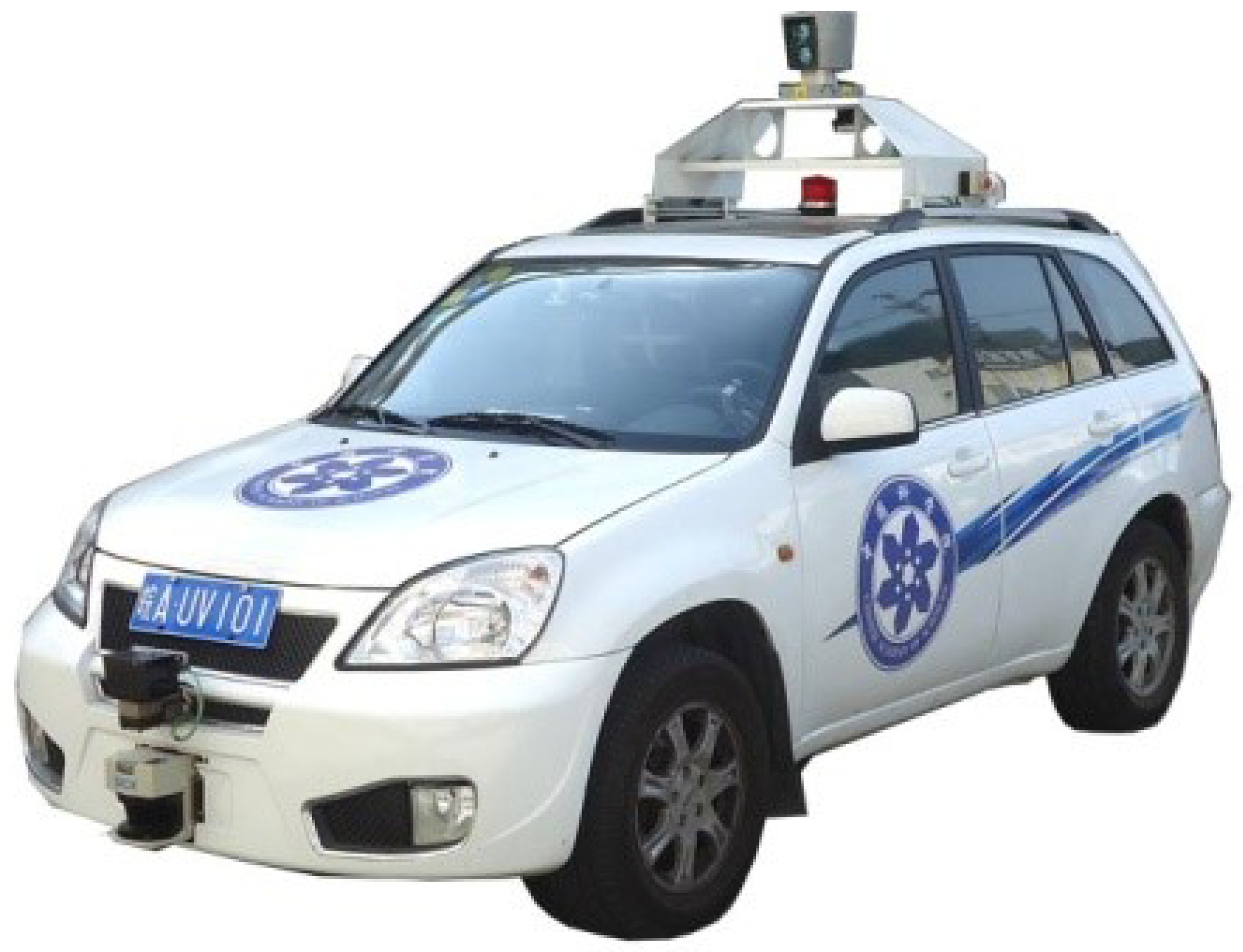
The experimental part will be based on the autonomous driving platform “Intelligent Pioneer”, developed by the Hefei Institute of Physical Science, Chinese Academy of Sciences. As shown in Figure 10, the platform is equipped with a 128-line LiDAR, a high-precision integrated navigation system, a wheel odometer and other sensors.

3.2. LiDAR Double Constraint Verification Experiment

This section will verify the effect of the LiDAR constraint. Similar to mainstream 3D LiDAR odometry, the LiDAR constraint introduced in this paper is the registration constraint of two point clouds, but this paper adds the LiDAR constraint to the sliding window. Based on the sensor fusion framework, two constraints are specified: the binary edge constraint inside the window and the unary edge constraint outside the window, which correspond to the scan-to-scan constraint and scan-to-map constraint of the LiDAR, respectively. The marginalization constraint of the sliding window will also be added to the fusion framework as a prior constraint, so the main purpose of this experiment is to verify the correctness of the multi-sensor fusion framework and verify the multi-frame point cloud registration in the constraint within the window. Comparisons of real-time performance, accuracy and algorithm time costs between this scheme and mainstream LiDAR odometry will be performed.
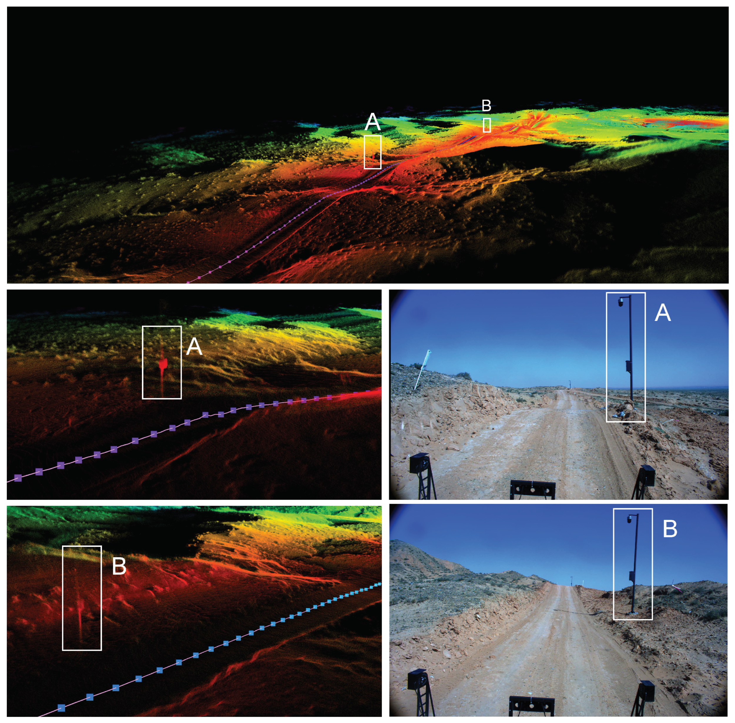
We select a typical off-road environment and use an Intel i7-9700 CPU to conduct the experiments. In this paper, we set the number of sliding window variables to three. The resulting mapping effect is shown in Figure 11. We can see that the details of the markers are all in the figure. Using the mainstream LiDAR odometry LOAM and LeGO-LOAM to conduct experiments under the same conditions, the obtained mapping effects are shown in Figure 12. We can verify the correctness of the LiDAR constraints in the fusion framework in this paper, and compared with other mainstream LiDAR odometers, the solution in this paper also has a greater advantage in clarity.
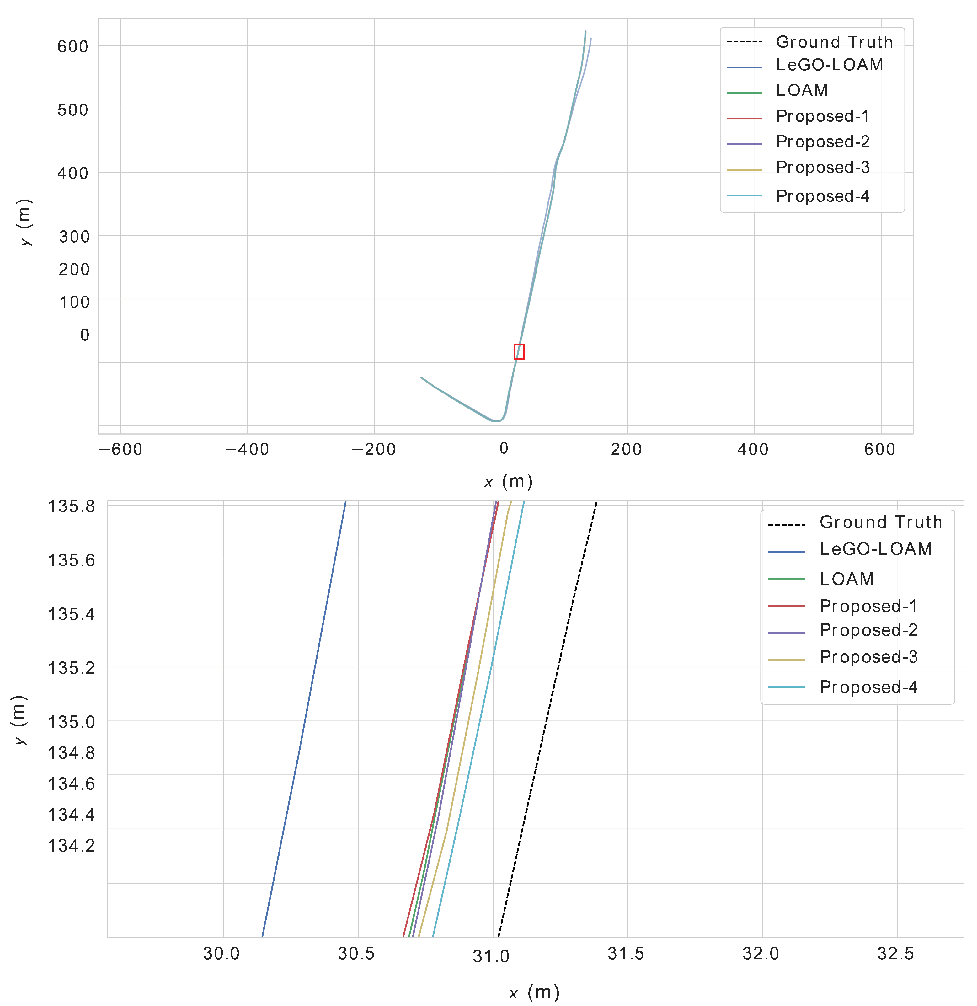
For quantitative analysis, the pose output of the combined navigation is taken as the ground truth. Figure 13 shows the experimental trajectories of each system, where “Proposed-n” is the LiDAR constraint scheme in this paper, and n represents the number of variables inside the sliding window. The amount of point cloud data is very large, and too many variables in the sliding window will be very time-consuming, so the maximum number of window variables in the experiment is set to four.
Table 1 summarizes the errors of each track in Figure 13, and Table 2 shows the average time spent processing a single keyframe for each track. For the calculation of the average time, the solution in this paper selects all the time for the construction and solution of the graph optimization problem, LOAM selects the single-frame solution time in its LaserMapping process and LeGO-LOAM selects the scan-to-map single-frame solution time. It can be found that LOAM cannot run in real time under the data volume of 128 lines. Although LeGO-LOAM has the fastest solution speed, the error is relatively high. As the sliding window variables increase in the framework of this paper, the system solution will take more and more time. However, the accuracy can also be improved. Accordingly, under the comprehensive comparison of solution time and accuracy, the scheme in this paper has more advantages.

3.3. Occupancy Grid Map

Figure 14 is the grid map and its corresponding satellite map generated by the algorithm in this paper, and Figure 15 is the overlay display of the probability grid map and the point cloud map, in which the left part of the point cloud map cancels its display. Zoom in to see that the obstacles are correctly marked in the occupancy grid map (dark green is the unknown area, light gray is the passable area, black is the obstacle area).
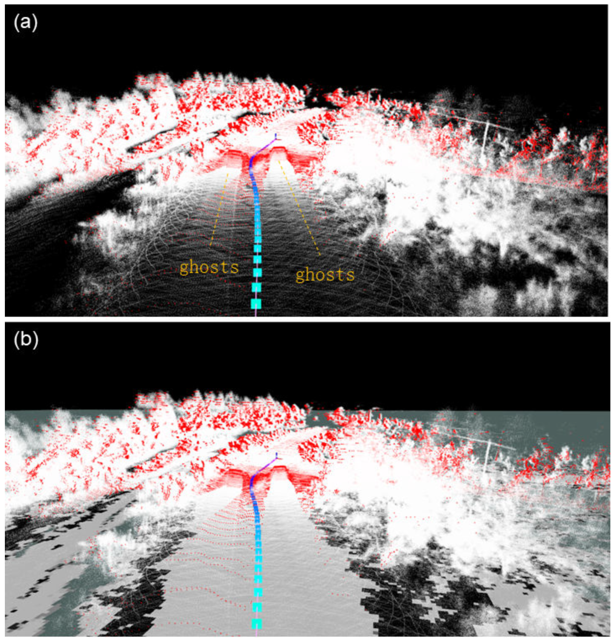
Since this paper uses multi-frame data to update the grid map, the dynamic obstacles can be effectively removed at the level of the two-dimensional grid map. Therefore, through the performance of dynamic obstacles in the occupied grid map, it is easy to verify the correctness of multi-frame data fusion. As shown in Figure 16, the point cloud map is constructed and represented in white, and the LiDAR point cloud data of the current frame is represented in red. It can be observed in (a) that two moving vehicles follow the experimental vehicle in the back. Due to the driving of these two vehicles, a long ghost image is left on the point cloud map (because the point cloud map is a multi-frame stitching, and the two vehicles are moving). Compared with (a), only the visualization of the occupied grid map is turned on in (b). It can be seen that the multi-frame update strategy in this paper enables these dynamic obstacles to be eliminated at the two-dimensional grid map level. However, if only the point cloud is projected directly into the grid map, these “ghosts” are bound to be seen as obstacles.

3.4. Enhanced Registration

This section verifies the feedback effect of the grid map. In an environment with dynamic obstacles, we verify the effectiveness of adding the “enhanced registration” of the grid map and removing the dynamic obstacles in the point cloud map.
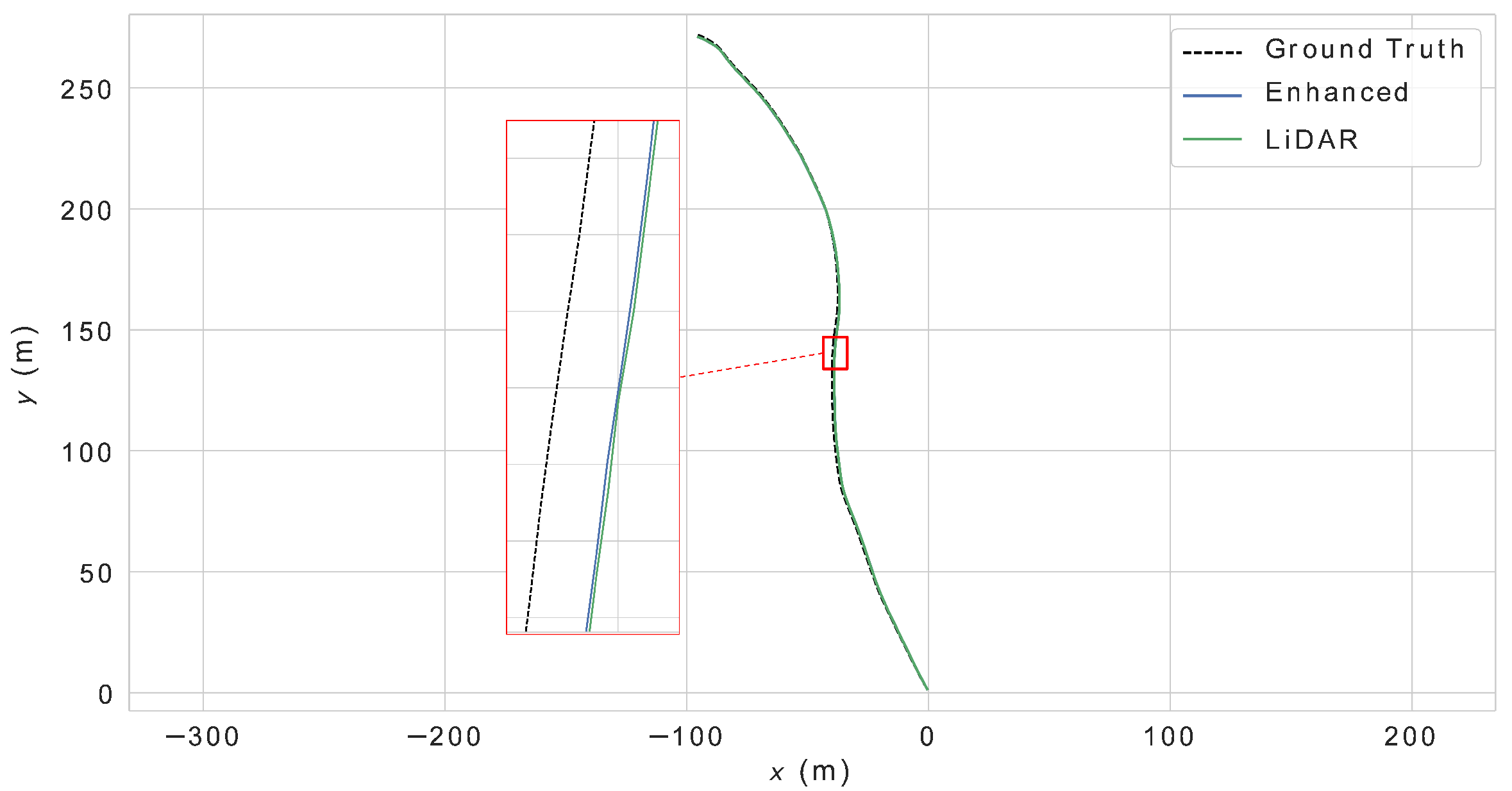
In the previous section, dynamic obstacles were removed at the grid map level because the grid map is the fusion result of all historical frames. So, in the residual error outside the LiDAR window, the “binary” semantics of the grid map can be borrowed to weight the point cloud registration. This experiment continues in the dynamic obstacle scene in the previous section. Figure 17 contains the projected grid map of a single point cloud frame (white for non-obstacles, black for obstacles, gray for unknown area) and the virtual single-frame occupancy grid map generated by using the global occupancy grid map (from white to black corresponding to the occupancy probability from small to large). We can see the dynamic obstacles in the virtual grid map (the back of Figure 16). The two moving vehicles have been removed, and the binary “semantics” corresponding to the projection image of a single frame of the point cloud are inconsistent. Thereby, the registration weight will be greatly reduced and effectively improve the registration accuracy. Figure 18 shows the use of LiDAR. We constrain and add the trajectories before and after “enhanced registration”. Table 3 shows their trajectory errors. It can be found that the “enhanced registration” proposed in this paper can significantly reduce the average error and root mean square error of the system. Therefore, the effectiveness of this scheme can be proven.

4. Discussion

By abstracting the registration constraints of LiDAR into in-window constraints and out-of-window constraints, the in-window constraints can be adjusted in conjunction with multiple frames to improve registration accuracy when there are fewer feature points. The out-of-window constraints have rich point cloud information. However, its variables are no longer involved in the optimization and also provide a lot of information through the enhanced registration of the grid map. By comparing with the mainstream LiDAR SLAM solutions LOAM and LeGO-LOAM, our solution has advantages in trajectory accuracy and map details, and provides a foundation for the multi-sensor fusion solution. We will expand it to more sensor fusion paradigms. Although our method has been able to solve some problems, the current disadvantage is that LiDAR is still a relatively low-frequency sensor, and different environmental characteristics can lead to a large gap in localization accuracy. In the future, we will consider the fusion of multiple sensors to improve the absolute reliability of the entire localization system.

5. Conclusions

In this paper, a dual-constrained LiDAR SLAM scheme is proposed, which abstracts LiDAR registration into in-window constraints and out-of-window constraints, so that our scheme can compromise between accuracy and real-time performance. Although the variables outside the window no longer participate in the optimization process. In this paper, we can also provide binary semantic information by using a two-dimensional probability grid map and provide dynamic weights for out-of-window constraints, so as to achieve the effect of enhancing the registration accuracy. Finally, we conducted experiments such as double-constraint verification, grid map construction and enhanced registration effect verification in an off-road environment and compared our results with the mainstream LiDAR SLAM schemes LOAM and LeGO-LOAM, proving that the scheme in this paper has more advantages. In the future, visual sensor constraints will be added to better adapt to certain extreme environments. In summary, this paper has completed research on SLAM technology for off-road environments and has conducted several real-world experiments in off-road environments with good results, providing an effective solution for automatic driving localization and map building in off-road environments.

Author Contributions

Conceptualization, H.Z. and X.K.; methodology, H.Z.; software, X.K. and Z.C.; validation, H.Z. and T.S.; formal analysis, H.Z. and X.K.; investigation, T.S. and B.L.; data curation, Z.C. and B.L.; writing—original draft preparation, X.K.; writing—review and editing, B.Y. and B.L.; visualization, T.S.; supervision, H.Z.; project administration, H.Z.; funding acquisition, H.Z. All authors have read and agreed to the published version of the manuscript.

Funding

This work was supported partially by the Youth Innovation Promotion Association of the Chinese Academy of Sciences (Grant No. Y2021115).

Institutional Review Board Statement

Not applicable.

Informed Consent Statement

Not applicable.

Data Availability Statement

Some data presented in this study are available on request from the corresponding author. The data are not publicly available due to the confidentiality clause of some projects.

Conflicts of Interest

The authors declare no conflict of interest.

References

  1. Cadena, C.; Carlone, L.; Carrillo, H.; Latif, Y.; Scaramuzza, D.; Neira, J.; Reid, I.; Leonard, J.J. Past, Present, and Future of Simultaneous Localization and Mapping: Toward the Robust-Perception Age. IEEE Trans. Robot. 2016, 32, 1309–1332. [Google Scholar] [CrossRef] [Green Version]
  2. Arun, K.S.; Huang, T.S.; Blostein, S.D. Least-Squares Fitting of Two 3-D Point Sets. IEEE Trans. Pattern Anal. Mach. Intell. 1987, PAMI-9, 698–700. [Google Scholar] [CrossRef] [PubMed] [Green Version]
  3. Biber, P.; Strasser, W. The normal distributions transform: A new approach to laser scan matching. In Proceedings of the 2003 IEEE/RSJ International Conference on Intelligent Robots and Systems (IROS 2003) (Cat. No.03CH37453), Las Vegas, NV, USA, 27–31 October 2003; Volume 3, pp. 2743–2748. [Google Scholar] [CrossRef]
  4. Kohlbrecher, S.; von Stryk, O.; Meyer, J.; Klingauf, U. A flexible and scalable SLAM system with full 3D motion estimation. In Proceedings of the 2011 IEEE International Symposium on Safety, Security, and Rescue Robotics, Kyoto, Japan, 1–5 November 2011; pp. 155–160. [Google Scholar] [CrossRef] [Green Version]
  5. Olson, E.B. Real-time correlative scan matching. In Proceedings of the 2009 IEEE International Conference on Robotics and Automation, Kobe, Japan, 12–17 May 2009; pp. 4387–4393. [Google Scholar] [CrossRef] [Green Version]
  6. Hong, S.; Ko, H.; Kim, J. VICP: Velocity updating iterative closest point algorithm. In Proceedings of the 2010 IEEE International Conference on Robotics and Automation, Anchorage, AK, USA, 4–8 May 2010; pp. 1893–1898. [Google Scholar] [CrossRef]
  7. Censi, A. An ICP variant using a point-to-line metric. In Proceedings of the 2008 IEEE International Conference on Robotics and Automation, Pasadena, CA, USA, 19–23 May 2008; pp. 19–25. [Google Scholar] [CrossRef] [Green Version]
  8. Zhang, J.; Singh, S. Low-Drift and Real-Time Lidar Odometry and Mapping. Auton. Robots 2017, 41, 401–416. [Google Scholar] [CrossRef]
  9. Lu, F.; Milios, E.E. Globally Consistent Range Scan Alignment for Environment Mapping. Auton. Robots 1997, 4, 333–349. [Google Scholar] [CrossRef]
  10. Gutmann, J.S.; Nebel, B. Navigation Mobiler Roboter Mit Laserscans. In Proceedings of the Autonome Mobile Systeme 1997, 13. Fachgespräch, Stuttgart, Germany, 6–7 October 1997; Springer: Berlin/Heidelberg, Germany, 1997; pp. 36–47. [Google Scholar]
  11. Shan, T.; Englot, B.; Meyers, D.; Wang, W.; Ratti, C.; Rus, D. LIO-SAM: Tightly-coupled Lidar Inertial Odometry via Smoothing and Mapping. In Proceedings of the 2020 IEEE/RSJ International Conference on Intelligent Robots and Systems (IROS), Las Vegas, NV, USA, 25–29 October 2020; pp. 5135–5142. [Google Scholar] [CrossRef]
  12. Kaess, M.; Johannsson, H.; Roberts, R.; Ila, V.; Leonard, J.; Dellaert, F. iSAM2: Incremental smoothing and mapping with fluid relinearization and incremental variable reordering. In Proceedings of the 2011 IEEE International Conference on Robotics and Automation, Shanghai, China, 9–13 May 2011; pp. 3281–3288. [Google Scholar] [CrossRef]
  13. Ye, H.; Chen, Y.; Liu, M. Tightly Coupled 3D Lidar Inertial Odometry and Mapping. In Proceedings of the 2019 International Conference on Robotics and Automation (ICRA), Montreal, QC, Canada, 20–24 May 2019; pp. 3144–3150. [Google Scholar] [CrossRef] [Green Version]
  14. Sibley, G.; Matthies, L.; Sukhatme, G. A Sliding Window Filter for Incremental SLAM; Springer: Boston, MA, USA, 2008; Volume 8 LNEE, pp. 103–112. [Google Scholar] [CrossRef]
  15. Ji, K.; Chen, H.; Di, H.; Gong, J.; Xiong, G.; Qi, J.; Yi, T. CPFG-SLAM:a Robust Simultaneous Localization and Mapping based on LIDAR in Off-Road Environment. In Proceedings of the 2018 IEEE Intelligent Vehicles Symposium (IV), Changshu, China, 26–30 June 2018; pp. 650–655. [Google Scholar] [CrossRef]
  16. Grisetti, G.; Stachniss, C.; Burgard, W. Improving Grid-based SLAM with Rao-Blackwellized Particle Filters by Adaptive Proposals and Selective Resampling. In Proceedings of the 2005 IEEE International Conference on Robotics and Automation, Barcelona, Spain, 18–22 April 2005; pp. 2432–2437. [Google Scholar] [CrossRef]
  17. Hess, W.; Kohler, D.; Rapp, H.; Andor, D. Real-time loop closure in 2D LIDAR SLAM. In Proceedings of the 2016 IEEE International Conference on Robotics and Automation (ICRA), Stockholm, Sweden, 16–21 May 2016; pp. 1271–1278. [Google Scholar] [CrossRef]
  18. Moravec, H. Sensor Fusion in Certainty Grids for Mobile Robots. AI Mag. 1988, 9, 61–74. [Google Scholar]
  19. Shan, T.; Englot, B. LeGO-LOAM: Lightweight and Ground-Optimized Lidar Odometry and Mapping on Variable Terrain. In Proceedings of the 2018 IEEE/RSJ International Conference on Intelligent Robots and Systems (IROS), Madrid, Spain, 1–5 October 2018; pp. 4758–4765. [Google Scholar] [CrossRef]
  20. Hornung, A.; Wurm, K.M.; Bennewitz, M.; Stachniss, C.; Burgard, W. OctoMap: An Efficient Probabilistic 3D Mapping Framework Based on Octrees. Auton. Robots 2013, 34, 189–206. [Google Scholar] [CrossRef] [Green Version]
  21. Chen, X.; Milioto, A.; Palazzolo, E.; Giguère, P.; Behley, J.; Stachniss, C. SuMa++: Efficient LiDAR-based Semantic SLAM. In Proceedings of the 2019 IEEE/RSJ International Conference on Intelligent Robots and Systems (IROS), Macau, China, 3–8 November 2019; pp. 4530–4537. [Google Scholar] [CrossRef]
Figure 1. The system framework is composed of in-window and out-of-window constraints: the in-window constraints are formed by the registration between frames and are associated with two poses, and the out-of-window constraints are formed by the registration of frames and subgraphs and are only associated with the in-window variables. However, the out-of-window constraint will add additional information from the 2D grid map to enhance the registration ability.
Remotesensing 14 05705 g001
Figure 2. The marginalization constraint of the sliding window, that is, the constraints associated with the variables to be thrown out of the window are integrated into the prior constraints of the variables in the window.
Remotesensing 14 05705 g002
Figure 3. Transform the line feature points of the k frame to the k − 1 frame and construct the point-line distance as the residual.
Remotesensing 14 05705 g003
Figure 4. Transform the surface feature points of the k frame to the k 1 frame and construct the point-surface distance as the residual.
Remotesensing 14 05705 g004
Figure 5. Transform the line feature points of the k frame to the world coordinate system and construct the point-line distance as the residual.
Remotesensing 14 05705 g005
Figure 6. Transform the surface feature points of the k frame to the world coordinate system and construct the point-surface distance as the residual.
Remotesensing 14 05705 g006
Figure 7. Mark laser points with slopes greater than the threshold as an obstacle point cloud.
Remotesensing 14 05705 g007
Figure 8. Project the obstacle point cloud into a grid map and mark the grids with point cloud height differences greater than a threshold as obstacle grids.
Remotesensing 14 05705 g008
Figure 9. We transform the global grid map into the pose of the current frame as a virtual grid map observation and perform semantic comparison with the currently observed grid map to weight the registration.
Remotesensing 14 05705 g009
Figure 10. Our experimental platform is mechanically stable, with a 128-line LiDAR, which can meet the experimental requirements.
Remotesensing 14 05705 g010
Figure 11. The map constructed by this solution can also have very clear map details in the off-road environment.
Remotesensing 14 05705 g011
Figure 12. In the same environment, we experiment with LOAM and LeGO-LOAM, and we can see that our scheme is more advantageous in terms of clarity.
Remotesensing 14 05705 g012
Figure 13. It can be seen from the experimental trajectory that our scheme has higher accuracy than LOAM and LeGO-LOAM, and the accuracy increases with the increase in the variables in the window.
Remotesensing 14 05705 g013
Figure 14. The constructed grid map is basically consistent with the outline of the satellite map and has very good detail on the passable markers.
Remotesensing 14 05705 g014
Figure 15. The two graphs represent the global graph and the enlarged graph of the selected point a respectively. A global graph is a superposition of a grid graph and a point cloud graph. An enlarged view of position A shows that obstacles at position A are correctly marked on the occupancy grid map (dark green for unknown areas, light gray for passable areas, and black for obstacles).
Remotesensing 14 05705 g015
Figure 16. On the 2D grid map level, ghosting can be effectively eliminated. In (a), there are two moving vehicles behind the experimental vehicle, which leave a long ghost shadow to the point cloud map due to the movement of these two vehicles. (b) only turns on the visualization of the occupied grid map more compared to (a), and it can be seen that the multi-frame update strategy in this paper makes these dynamic obstacles eliminated at the 2D grid map level.
Remotesensing 14 05705 g016
Figure 17. Corresponding to Figure 9, by generating a virtual single-frame grid map observation, semantic comparison with the current frame grid map is performed to weight the registration.
Remotesensing 14 05705 g017
Figure 18. It can be found that the enhanced registration scheme can further improve the trajectory accuracy in dynamic environments.
Remotesensing 14 05705 g018
Table 1. The translational part of the absolute trajectory error (m).
MethodMaximumAverageMedianMinimumRMSE
LOAM1.2010110.5912470.5686040.1297930.623795
L-LOAM 113.2316613.2607532.6254111.0943183.895525
Proposed10.9930790.4062580.4257930.0141400.445461
Proposed21.0058870.3863230.3904180.0192780.423526
Proposed31.0035200.3526820.3508410.0125320.394792
Proposed40.8660140.3447860.3188180.0133490.381943
1 LeGO-LOAM.
Table 2. Average solution time with different methods.
MethodLOAML-LOAM 1Proposed1Proposed2Proposed3Proposed4
Time (ms)8034.92166.872187.697218.506282.142380.868
1 LeGO-LOAM.
Table 3. Enhanced registration experimental trajectory error (m).
MaximumAverageMedianMinimumRMSE
LiDAR0.6424590.2427910.1918370.0557540.279967
Enhanced0.7349110.1872760.1548010.0251540.228453
Publisher’s Note: MDPI stays neutral with regard to jurisdictional claims in published maps and institutional affiliations.