Abstract
The spatial resolution of current soil moisture (SM) products is generally low, consequently limiting their applications. In this study, a deep belief network-based method (DBN) was used to downscale the Soil Moisture Active Passive (SMAP) L4 SM product. First, the factors affecting soil surface moisture were analyzed, and the significantly correlated ones were selected as predictors for the downscaling model. Second, a DBN model was trained and used to downscale the 9 km SMAP L4 SM to 1 km in the study area on 25 September 2019. Validation was performed using original SMAP L4 SM data and in situ measurements from SM and temperature wireless sensor network with 34 sites. Finally, the DBN method was compared with another commonly used machine learning model-random forest (RF). Results showed that (1) the downscaled 1 km SM data are in good agreement with the original SMAP L4 SM data and field measured data, and (2) DBN has a higher correlation coefficient and a lower root mean square error than those of RF. The coefficients of determination for fitting the two models with the measured data at the site were 0.5260 and 0.4816, with relative mean square errors of 0.0303 and 0.0342 m3/m3, respectively. The study also demonstrated the applicability of the DBN method to AMSR SM data downscaling besides SMAP. The proposed method can provide a framework to support future hydrological modeling, regional drought monitoring, and agricultural research.
1. Introduction
Soil moisture (SM) is a key factor in the surface water cycle, affecting the water–heat exchange in global surface processes [1,2]. It also has important effects on plant productivity, soil biology, geochemistry, and surface hydrology [3,4]. The surface SM product data estimated by satellite remote sensing technology have been widely used in drought monitoring and climate modeling [5,6]. However, its application in regional hydrology and agriculture is limited due to its low resolution, in which the spatial resolution of SM products needs to be at least 1 km [6,7]. Considerable effort has focused on developing SMD approaches to improve the spatial resolution of SM products retrieved from satellites [6,7,8,9,10,11,12].
Microwaves are particularly sensitive to moisture, have a certain penetrability to the surface, and are less affected by weather during data acquisition; thus, microwave remote sensing has always been highly valued in monitoring the SM of the continent. The most widely used SM products are the Advanced Microwave Scanning Radiometer(AMSR)-Earth Observing System SM, Soil Moisture and Ocean Salinity(SMOS) SM, and Soil Moisture Active Passive (SMAP) SM [7,8,9,10,11,12,13,14]. The feasibility and accuracy of these products have been verified for global application, but their resolutions are low, generally tens of kilometers [13,14,15,16,17,18,19,20,21,22]. If the coarse spatial resolution of SM product data can be improved by downscaling, then they will be more widely used.
Downscaling studies and products are well reviewed in the literature [6,7,8]. Various downscaling methods or algorithms can be divided into empirical [9,10,11,12,13,14,15,22,23,24,25,26,27,28,29,30,31,32], semi-empirical [33,34,35] and physical model based methods [36], of which the first method is the most widely used. The principle of the empirical downscaling method is that a model is first constructed based on coarse-scale SM data and high-resolution optical/infrared remote sensing data. Then, high-spatial resolution data, which are used as predictors, are input into the model to calculate the downscaled SM. The polynomial regression function is the most commonly used empirical spatial downscaling relational model. The high-resolution data used as predictors originate from optical and infrared remote sensing observations and usually include land surface temperature (LST) and vegetation index (VI) [29]. In addition, surface albedo (ALB), elevation and slope aspect, meteorological, evapotranspiration (ET), and radar data have also been used in downscaling studies [24,29,36,37].
In recent years, much progress has been attained in geoscience modeling by using artificial intelligence (AI), machine learning (ML), and deep learning (DL). DL is a subset of ML, and ML is a subclass of AI. Undeniably, advanced ML methods should be employed to solve problems in the earth sciences, as they enable researchers to solve many difficult problems [38]. Moreover, ML algorithms can describe the nonlinear relationship between SM and downscaling factors. Numerous researchers have attempted to downscale SM data based on ML by using the random forest (RF) [12,23,39], support vector machine, and artificial neural network [12,40,41]. These models have their own advantages and disadvantages, and their applicability is usually affected by the selection of training data, downscaling factors, and characteristics of study areas [8,12,39].
As DL methods can effectively discover more complex correlations between prediction variables and input coarse-scale SM data [38,42], researchers have also explored DL-based downscaling methods [39,43,44,45]. However, exploration in this area still needs to be developed. Therefore, a spatial DL-based method combined with the deep belief network (DBN) is presented in this study for downscaling SMAP SM data.
The purposes of this study are as follows: (1) select factors that affect SM variations via statistical analysis, which includes not only normalized difference vegetation index (NDVI) and LST but also other spatial information features, such as relevant band data in Landsat 8 OLI data, wetness index (WI) obtained from Landsat 8-based Tasseled-cap Transform, digital elevation model(DEM), slope and aspect, enhanced vegetation index (EVI), ALB, and leaf area index (LAI); (2) train and test DBN in downscaling SM; and (3) compare the performance of DL models with the RF model.
2. Materials and Methods
2.1. Study Area
The study area is located in the Shandian River Basin and surrounding watersheds in North China, within an area of approximately 10,000 km2 (115.5–116.5°E, 41.5–42.5°N) (Figure 1). It has a semi-arid continental climate, with a maximum inter-annual temperature of approximately 36 °C and a minimum temperature of approximately −36 °C [19]. The average annual rainfall and evaporation are approximately 375 and 1188 mm, respectively. Precipitation is concentrated in summer from June to September, accounting for more than 80% of the annual rainfall. Aeolian sandy soil is the main soil type, accounting for approximately 50% of the total area, followed by 8% meadow soil. The terrain of the basin is relatively flat and dominated by plains, hills, and depressions. The land cover types include farmland, forest, grassland, shrubs, wetlands, water bodies, residential land and bare land, of which the main types are farmland and grassland (Figure 1).
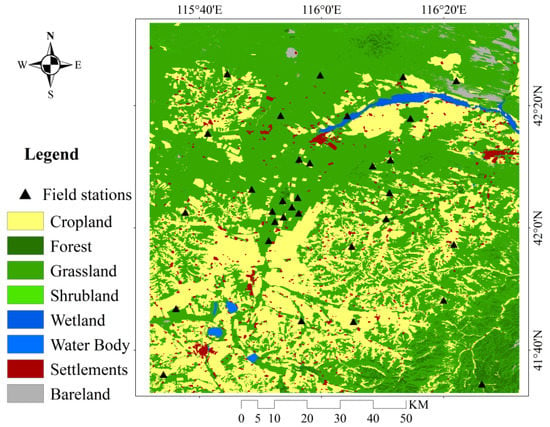
Figure 1.
Location and land cover type of the study area; Locations of 34 SMN-SDR stations noted (solid triangle).
2.2. Research Data
The research data include SMAP SM products, AMSR-2 SM products, MODIS data products, Landsat 8 OLI data, DEM elevation data, and SM field observation data, as listed in Table 1. The original format of SMAP L4-SM data and MODIS data is HDF and converted into TIFF format by using HEGTool (HDF-EOS and GeoTIFF conversion tools) from the National Aeronautics and Space Administration (NASA) and then reprojected. The Landsat data are preprocessed using the Google Earth engine (GEE) platform. All data are clipped to the size of the study area after their projections are ensured to be consistent with the coarse-scale SMAP and AMSR-2 data, and the water bodies of the images are masked.

Table 1.
Description of datasets used in this study.
2.2.1. In Situ Observations
In 2018, an SM and temperature wireless sensor network with 34 sites was established in the Shandian River Basin (SMN-SDR) [21,46]. The 34 sites (Figure 1) were designed according to three scales: 100 km (large scale), 50 km (medium scale), and 10 km (small scale) (http://data.tpdc.ac.cn/zh-hans/, accessed on 22 January 2022). At each station, the SM and soil temperature were measured at different measurement depths of 3, 5, 10, 20, and 50 cm [20]. As the measuring depth of SMAP L4 was 0–5 cm, the top 3 cm in situ measurements were used to verify the downscaled SM results.
2.2.2. Remotely Sensed SM Data
The remotely sensed SM data in this study were obtained from two passive microwave sensors, namely, AMSR-2 and SMAP. The AMSR-2 onboard the GCOM-W satellite was launched in May 2012 and was used to continue the Aqua/AMSR-E mission (http://suzaku.eorc.jaxa.jp/GCOM_W, accessed on 7 May 2022). The AMSR-2 L2 data with a spatial resolution of 10 km and dated 25 September 2019 were downloaded from NASA (https://earthdata.nasa.gov/, accessed on 7 May 2022).
Launched in 2015, SMAP is the latest satellite specially designed by NASA to monitor SM by using the L-band, and it is considered to be the most sensitive band for SM sensing. The good performance of the SMAP SM product has been confirmed by multiple studies [16,47,48,49].
SMAP Level 4 products are model-derived data of the surface and root zone SM in accordance with the SMAP Handbook, with a spatial resolution of 9 km and a temporal resolution of 3 h (https://nsidc.org/data/smap, accessed on 1 February 2022). The SMAP L4-SM data on 25 March, 25 May, 25 September, and 25 November 2019 were downloaded and preprocessed. Among them, the SMAP L4-SM data on 25 September were used to build the downscaling model, and the SM data on other dates were used to verify the temporal validity of the model.
2.2.3. MODIS Data
The MODIS data products used in this study include LST (MOD11A2), VI (MOD13A2), ALB (MCD43A3), LAI (MCD15A2), and ET (MOD16A2) (https://modis.gsfc.nasa.gov/, accessed on 8 February 2022). The independent variables of LST, NDVI (extracted from MOD13A2), EVI (extracted from MOD13A2), ALB, LAI, and ET in the study area were obtained from the datasets, and all of them were resampled to 9 and 10 km by using the nearest-neighbor method.
2.2.4. Topographic Data
DEM is a visual representation of ground elevation information, and other terrain factors, such as slope and aspect, can be obtained from DEM. The DEM data (GETED2010) used in this study was obtained from USGS and the US National Geospatial-Intelligence Agency. GMTED has three different resolutions: 30 arc seconds (about 1 km), 15 arc seconds (about 500 m), and 7.5 arc seconds (about 250 m). The 30 arc-second resolution GMTED data were used to extract the slope and aspect.
2.2.5. Landsat 8 OLI Data
The Landsat 8 images of the study area from September 2019 to October 2019 were downloaded in batches by using the GEE platform, with a spatial resolution of 30 m (https://code.earthengine.google.com/, accessed on 30 January 2022). In addition to the original Landsat band data, the wet index (WI) was obtained via tasseled cap transformation and then used as an independent variable for soil moisture downscaling.
2.3. Proposed Methodology
The flowchart of the overall methodology is shown in Figure 2. The main steps are as follows:
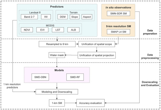
Figure 2.
Flowchart of the study.
Step 1: Determine the environmental factors affecting SM and then prepare training and test datasets for the model.
Step 2: Construct the DBN model and RF model. Evaluate the performance of the models by analyzing the degree of agreement between the downscaled SM and in situ observation data and original SMAP L4 SM data.
2.3.1. Selection of Predictors
The correlation between each affecting factor and the SMAP L4-SM data on 25 May, and 25 September were calculated. Table 2 shows ALB, ET, Slope aspect, LST and selected Landsat 8 OLI’s bands are negatively correlated with SM. By contrast, DEM, slope, NDVI, EVI, WI, and LAI are positively correlated with SM. Each factor is correlated with SM at a significant level of 0.01. Therefore, the red, green, blue, near-infrared, and short-wave infrared bands of Landsat 8 OLI, DEM, NDVI, LST, EVI, WI, LAI, ALB_vis, and ALB_nir were used as the downscaling predictors.

Table 2.
Correlation of factors.
2.3.2. DBN-Based Method
DBN Model
DBN is a DL network formed by stacking multiple Restricted Boltzmann machines (RBMs) and a backpropagation (BP) neural network (Figure 3a). When the correlation between the input data is unknown, it can learn and construct a nonlinear relationship between the input and output by referring to the feature values and labels of the input dataset. DBN can also rearrange shallow features into deeper abstract features so that more complex associations between features can be further excavated. The RBM in DBN consists of a visible layer (visible unit) and a hidden layer (hidden unit), as shown in Figure 3b. The output of the hidden layer of the previous layer of RBM is input into the next layer of RBM, and this task is repeated several times. The output of the last RBM is input to the following BP layer. The middle layers of the RBM are fully connected, while the adjacent layers are not connected to each other [50].

Figure 3.
Structure of the DBN model (a) and RBM (b).
DBN-Based Downscaling Procedure
A DBN-based downscaling model between the predictors and SM was established and named Soil Moisture Downscaling-Deep Belief Network (SMD-DBN). Figure 4 shows the model structure.
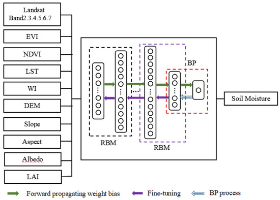
Figure 4.
SMD-DBN structure.
The procedure of constructing the SMD-DBN model can be described as follows.
The resampled low-resolution predictors and SMAP SM data are used as the training set to train the DBN model. The training process of the SMD-DBN model includes RBM pre-training and BP neural network back-propagation process. In the pre-training, an unsupervised method is used to train each layer of RBM. The training process can be regarded as a process of updating the weights and biases of the model. The pre-processed data are input into the visible layer of the RBM, and the activation function is used to pass the input data to the hidden layer to update the weights and biases by using the Gibbs sampling contrast divergence algorithm. The BP process refers to the process of fine-tuning the weights and biases. In the BP neural network, the Smooth L1 function is used as the loss function to prevent the gradient from exploding during model training.
Both training accuracy and training speed are taken into account in the network training. Some key parameter settings and results during the experiment are shown in Table 3. Multiple experiments are required to determine the training parameters, including the DBN hidden layer structure (hidden_layers_structure), number of sampling iterations of the contrastive divergence algorithm (cd_k), number of RBM iterations (RBM_epochs), RBM learning rate (RBM_learning_rate), number of BP algorithm iterations (BP_epochs), BP algorithm learning rate (BP_learning_rate), training sample batch (batch_size), and the drop factor (dropout). The final parameter settings are shown in Table 4.

Table 3.
Training parameters and results of the SMD-DBN model.

Table 4.
Training parameters of the SMD-DBN model.
After a trained model is obtained, the high-resolution predictors (1 km) are input into the trained model to obtain the predicted high-resolution SM data.
2.3.3. Evaluation Method
Three statistical metrics, namely, Pearson correlation coefficient (R), determination coefficient (R2), and root mean square error (RMSE), were used in the performance evaluation of the method. R and R2 were used to evaluate the correlation and fitting effect between the downscaling results and the original data or field measured data, respectively. RMSE was used to evaluate the error of the downscaling results.
3. Results and Discussion
3.1. Evaluation of the SMD-DBN-Downscaled SM Data
3.1.1. Evaluation with Original SM and Field Measurement
A comparison between the downscaling of 1 km SM (Figure 5b) and original 9 km SMAP SM data (Figure 5a) is shown in Figure 5. The blank part in Figure 5b represents the result of using the water mask. Compared with the original coarse-scale SMAP SM, the downscaled SMAP SM can maintain the consistency of the spatial variations of the original SM and provide more detailed spatial information. Figure 6a shows the scatter diagram and quantitative evaluation of the downscaled SM and its comparison with the original SMAP SM at the SMN-SDR sites. The R, R2, and RMSE between the downscaled SM and original SMAP L4 data are 0.8357, 0.6984, and 0.0210 m3/m3, respectively.
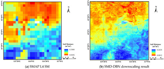
Figure 5.
Comparison of downscaling result and original SM data.
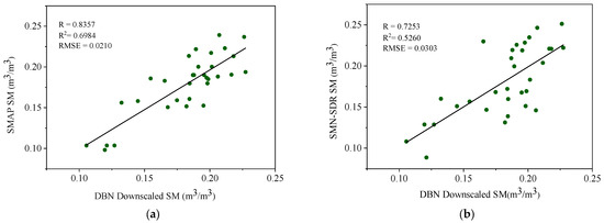
Figure 6.
Scatter plot of SM from DBN downscaling versus original SMAP SM data (a) and SMN-SDR in situ measurements (b).
Then, the downscaled SM result was verified with in situ SMN-SDR SM data. Figure 6b shows the scatter diagram and quantitative evaluation of the downscaled SM and its comparison with SMN-SDR in situ measurements. The R, R2, and RMSE between the downscaled SM and field measurements are 0.7253, 0.5260, and 0.0303 (m3/m3), respectively. The results indicate that the downscaled result is in good agreement with the field measurements. Compared with other downscaled SM products at 1 km resolution as reviewed previously [6,7], SMD-DBN outperforms most similar methods, with their R and RMSE values ranging from 0.41–0.73 and 0.049–0.131 (m3/m3). The accuracy of SMD-DBN also exceeds that of a comparable approach used in the same study area, which downscaled 9 km SMAP SM data to 1 km by using MODIS product (surface temperature and normalized VI) data and an adaptive window downscaling method [14].
3.1.2. Temporal Validation
The data date used for the training and validation of the SMD-DBN model are those pertaining to 25 September 2019. In view of exploring the application performance of the SMD-DBN model at other times, three different non-adjacent sites on different dates were selected for evaluation. The selected dates were 25 March, 25 May, 25 July and 25 November 2019, forming a time series with an interval of two months starting from 25 September when the model was established. The three stations are S2, M5, and L6, with the same naming convention as the original experiment [20,41], where S, M, and L represent the three scales of SMN-SDR, i.e., small, medium, and large sampling scales. Figure 7b,d,f,h are the downscaling results of the SMD-DBN model. Figure 7a,c,e,g are the original images of the low-resolution SMAP L4 SM product. The dates when the images were taken are 25 March, 25 May, 25 July and 25 November 2019, respectively.
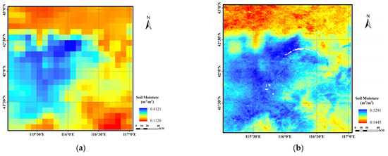
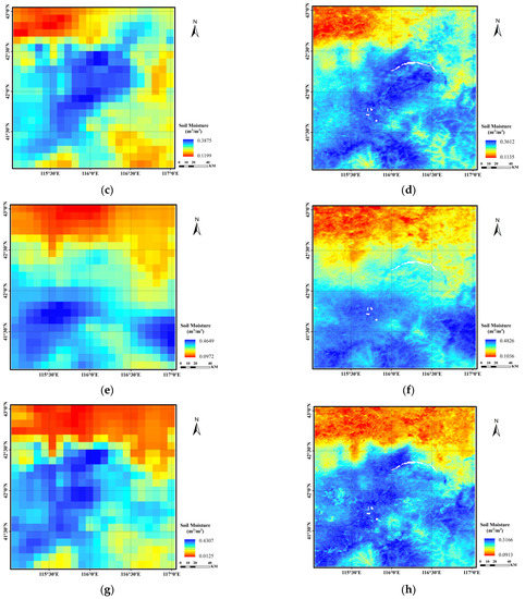
Figure 7.
Comparison of original SMAP SM data (a,c,e,g) and corresponding downscaling result (b,d,f,h) of different dates (25 March, 25 May, 25 July and 25 November 2019, note: white part is a result of using the water mask).
Figure 8 shows a comparison of the time-series SM of the SMD-DBN model downscaling results, original SMAP L4 data, and field measurements at S2, M5, and L6 stations. In contrast to the trend of the original SMAP L4 data, the changing trend of SM in the time series obtained by the SMD-DBN downscaling model is more consistent with that of the field measured data.

Figure 8.
Time series SM data of station L6 (a), M5 (b), and S2 (c).
For the quantitative performance evaluation of the model in time series, the mean absolute error (MAE) and mean relative error (MRE) between the downscaled results at three stations and the corresponding original SMAP and field measured values of SMN-SDR were calculated, respectively. As shown in Table 5, the MAE between downscaled SM and SMN-SDR field-measured SM for the three stations (L6, M5, and S2) range from 0.0161 to 0.0257, with an average of 0.0207. The accuracy of the model downscaling results does not fluctuate considerably over time.

Table 5.
Evaluation of downscaling results of time series.
3.2. Evaluation of SMD-DBN against SMD-RF
The RF algorithm is an integrated ML algorithm, and it can simulate the complex nonlinear relationship between independent variables and dependent variables [51]. Many previous studies have shown the suitability of RF algorithms for downscaling satellite products compared with other ML methods [13,52,53,54,55,56]. Here, an SMD-RF model was established to compare it with SMD-DBN. In particular, a nonlinear functional relationship between the input feature variables and output SM was established based on multiple decision trees, and the predictors used in the SMD-DBN model were used in the RF model. The expression of SMD-RF is given by
For the SMD-RF model, five parameters need to be optimized: iteration times (n_estimators), tree depth (max_depth), minimum sample number of leaf nodes (MIN_samples_split), minimum number of leaves required to split internal nodes (min_samples_leaf), and maximum number of features used by each tree (max_features). The final values of each parameter are shown in Table 6.

Table 6.
Parameters of SMD-RF model.
Figure 9 shows the downscaled SM from the SMD-RF model. Compared with the original SMAP SM data (Figure 5b), the downscaling results of SMD-DBN and SMD-RF models can both provide more detailed spatial information; however, while they have similar trends, their local effects differ from each other.
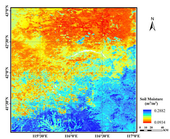
Figure 9.
Downscaled SM from SMD-RF (note: white part is a result of using the water mask).
The data and method used to verify the SMD-RF model are the same as those of the SMD-DBN model. A performance comparison between SMD-DBN and SMD-RF is shown in Table 7 and Figure 10.

Table 7.
Accuracy evaluation of the two models.
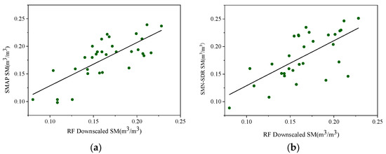
Figure 10.
Scatter plot of SM from SMD-RF downscaling versus original SMAP SM data (a) and SMN-SDR in situ measurements (b).
According to Table 8, SMD-DBN has a higher correlation with the in situ data (R) and smaller error of prediction results (RMSE), indicating its higher accuracy and better consistency with the original data compared with SMD-RF. Furthermore, Figure 10 shows a higher dispersion degree of SMD-RF than that of SMD-DBN (Figure 6).

Table 8.
Comparison of the SMD-DBN downscaling result with original AMSR-2 SM and in situ measurement data.
3.3. Transfer of SMD-DBN to AMSR-2
In this study, the AMSR-2 SM product was selected to explore the applicability of the SMD-DBN downscaling model to other data types. Figure 11 shows the downscaling results of AMSR-2 SM products based on the SMD-DBN model, in which (a) represents the original AMSR-2 image in the study area, and (b) represents the downscaling results of the SMD-DBN model. The quantitative evaluation result is listed in Table 8.
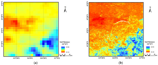
Figure 11.
Original AMSR-2 SM data (a) and SMD-DBN downscaling result (b).
The results showed that the downscaling results of AMSR-2 products have a high correlation with the original data (R = 0.8265, R2 = 0.6831, RMSE = 0.0257 m3/m3), proving the effectiveness of SMD-DBN model in downscaling the AMSR-2 SM products. However, the accuracy of AMSR-2′s downscaling results is much lower than that of SMAP (R = 0.5356, R2 = 0.2631, RMSE = 0.0321 m3/m3). The deviation of AMSR-2 data from in situ measurements may be attributed to the shallow penetration depth of the C/X band used in AMSR-2 and the errors in auxiliary information [16,21,57].
4. Conclusions
Microwave sensor-based SMs are widely used because data acquisition is rarely affected by atmospheric conditions, vegetation disturbances, and day–night cycles, but the low resolution limits their application. Aiming at the practical needs of SM products with high spatial resolution, this study presents the SMD-DBN model based on a deep confidence network, improving the SMAP L4 SM data resolution from 9 to 1 km. In situ observations from the new SM and temperature wireless sensor network (i.e., SMN-SDR) were used to evaluate the performance of SMD-DBN.
The main conclusions are as follows:
- (1)
- In terms of R, R2, and RMSE, the results obtained by the SMD-DBN model are in good agreement with the SMN-SDR field measurements, both spatially and temporally. The high spatial resolution SM map generated by this method has finer spatial information than the coarse resolution dataset and is highly consistent with the original SM data.
- (2)
- Compared with the widely used RF model, the proposed SMD-DBN model showed higher predictive performance when evaluated against SMN-SDR monitoring observations.
- (3)
- The downscaling method in this study can be applied to other coarse spatial scale remotely sensed SM dataset, such as AMSR-2. The SMD-DBN model has a good effect on the downscaling of SM product data, including SMAP and AMSR-2.
The results of this study confirm the ability of the proposed method to effectively provide high-resolution SM. As the SMAP L4 product provides SM data at a three-hour time resolution on a global 9 km grid, the proposed method can obtain SM maps with high spatial and temporal resolution. However, as near-infrared and visible remote sensing are easily affected by cloud cover, some predictors (e.g., VI) cannot be obtained sometimes, and downscaling models cannot be established. Future work can focus on solving the problem of missing data caused by cloud coverage and similar factors to obtain downscaled SM.
Author Contributions
Conceptualization, Y.C.; methodology, P.F., S.L. and M.L.; validation, Y.M.; investigation, A.L.; writing—original draft preparation, Y.C. and P.F.; writing—review and editing, Y.C., P.F., S.L. and M.L.; funding acquisition, A.L. All authors have read and agreed to the published version of the manuscript.
Funding
This research was partially funded by China Major Science and Technology Project of Natural Resources (Grant no. 121133000000190000).
Data Availability Statement
Enquiries about data availability should be directed to the authors.
Acknowledgments
Thanks are given to the International Soil Moisture Network and the National Tibetan Plateau/Third Pole Environment Data Center for providing in-situ soil moisture data. They are available for all users free of charge.
Conflicts of Interest
The authors declare no conflict of interest.
References
- Srivastava, P.K. Satellite Soil Moisture: Review of Theory and Applications in Water Resources. Water Resour. Manag. 2017, 31, 3161–3176. [Google Scholar] [CrossRef]
- Babaeian, E.; Sadeghi, M.; Jones, S.B.; Montzka, C.; Vereecken, H.; Tuller, M. Ground, proximal, and satellite remote sensing of soil moisture. Rev. Geophys. 2019, 57, 530–616. [Google Scholar] [CrossRef]
- Seneviratne, S.I.; Corti, T.; Davin, E.L.; Hirschi, M.; Jaeger, E.B.; Lehner, I.; Orlowsky, B.; Teuling, A.J. Investigating soil moisture-climate interactions in a changing climate: A review. Earth-Sci. Rev. 2010, 99, 125–161. [Google Scholar] [CrossRef]
- McColl, K.A.; Alemohammad, S.H.; Akbar, R.; Konings, A.G.; Yueh, S.; Entekhabi, D. The global distribution and dynamics of surface soil moisture. Nat. Geosci. 2017, 10, 100–104. [Google Scholar] [CrossRef]
- Agha Kouchak, A.; Farahmand, A.; Melton, F.S.; Teixeira, J.; Anderson, M.C.; Wardlow, B.D.; Hain, C.R. Remote sensing of drought: Progress, challenges and opportunities. Rev. Geophys. 2015, 53, 452480. [Google Scholar]
- Peng, J.; Loew, A.; Merlin, O.; Verhoest, N.E.C. A review of spatial downscaling of satellite remotely sensed soil moisture. Rev. Geophys. 2017, 55, 341–366. [Google Scholar] [CrossRef]
- Sabaghy, S.; Walker, J.P.; Renzullo, L.J.; Akbar, R.; Chan, S.; Chaubell, J.; Das, N.; Dunbar, R.S.; Entekhabi, D.; Gevaert, A.; et al. Comprehensive analysis of alternative downscaled soil moisture products. Remote Sens. Environ. 2020, 239, 1115856. [Google Scholar] [CrossRef]
- Zhao, W.; Wen, F.P.; Cai, J.F. Methods, progresses and challenges of passive microwave soil moisture spatial downscaling. Natl. Remote Sens. Bull. 2022, 26, 1699–1722. [Google Scholar] [CrossRef]
- Portal, G.; Vall-Llossera, M.; Piles, M.; Camps, A.; Chaparro, D.; Pablos, M.; Rossato, L. A spatially consistent downscaling approach for SMOS using an adaptive moving window. IEEE J. Sel. Top. Appl. Earth Obs. Remote Sens. 2018, 11, 1883–1894. [Google Scholar] [CrossRef]
- Zhao, W.; Nilda, S.; Lu, H.; Li, A. A spatial downscaling approach for the SMAP passive surface soil moisture product using random forest regression. J. Hydrol. 2018, 563, 1009–1024. [Google Scholar] [CrossRef]
- Dandridge, C.; Fang, B.; Lakshmi, V. Downscaling of SMAP Soil Moisture in the Lower Mekong River Basin. Water 2019, 12, 56. [Google Scholar] [CrossRef]
- Liu, Y.; Jing, W.; Wang, Q.; Xia, X. Generating high-resolution daily soil moisture by using spatial downscaling techniques: A comparison of six machine learning algorithms. Adv. Water Resour. 2020, 141, 103601. [Google Scholar] [CrossRef]
- Hu, F.; Wei, Z.; Zhang, W.; Dorjee, D.; Meng, L. A spatial downscaling method for SMAP soil moisture through visible and shortwave-infrared remote sensing data. J. Hydrol. 2020, 590, 125360. [Google Scholar] [CrossRef]
- Wen, F.P.; Zhao, W.; Hu, L.; Xu, H.X.; Cui, Q. SMAP passive microwave soil moisture spatial downscaling based on optical remote sensing data: A case study in Shandian river basin. Natl. Remote Sens. Bull. 2021, 25, 962–973. [Google Scholar]
- Warner, D.L.; Guevara, M.; Callahan, J.; Vargas, R. Downscaling satellite soil moisture for landscape applications: A case study in Delaware, USA. J. Hydrol. Reg. Stud. 2021, 38, 100946. [Google Scholar] [CrossRef]
- Cui, H.; Jiang, L.; Du, J.; Zhao, S.; Wang, G.; Lu, Z.; Wang, J. Evaluation and analysis of AMSR-2, SMOS, and SMAP soil moisture products in the Genhe area of China. J. Geophys. Res. Atmos. 2017, 122, 8650–8666. [Google Scholar] [CrossRef]
- Zeng, J.; Chen, K.S.; Bi, H.; Chen, Q. A preliminary evaluation of the SMAP radiometer soil moisture product over United States and Europe using ground-based measurements. IEEE Trans. Geosci. Remote Sens. 2016, 54, 4929–4940. [Google Scholar] [CrossRef]
- Zhang, X.; Zhang, T.; Zhou, P.; Shao, Y.; Gao, S. Validation analysis of SMAP and AMSR2 soil moisture products over the United States using ground-based measurements. Remote Sens. 2017, 9, 104. [Google Scholar] [CrossRef]
- Xie, Q.X.; Jia, L.; Chen, Q.T.; Yin, Y.M.; Massimo, M. Evaluation of microwave remote sensing soil moisture products in farming-pastoral area of Shandian river basin. Natl. Remote Sens. Bull. 2021, 25, 974–989. [Google Scholar]
- Wang, X.; Lü, H.; Crow, W.T.; Zhu, Y.; Wang, Q.; Su, J.; Zheng, J.; Gou, Q. Assessment of SMOS and SMAP soil moisture products against new estimates combining physical model, a statistical model, and in-situ observations: A case study over the Huai River Basin, China. J. Hydrol. 2021, 598, 126468. [Google Scholar] [CrossRef]
- Zheng, J.; Zhao, T.; Lü, H.; Shi, J.; Cosh, M.H.; Ji, D.; Jiang, L.; Cui, Q.; Lu, H.; Yang, K.; et al. Assessment of 24 soil moisture datasets using a new in situ network in the Shandian River Basin of China. Remote Sens. Environ. 2022, 271, 112891. [Google Scholar] [CrossRef]
- Meng, Y.; Wang, D.; Lin, Y.; Du, Y.; Zhang, Z.; Wang, D.; Lin, Z. Comparative evaluation and difference analysis of SMOS and SMAP satellite remote sensing soil moisture products. Acta Sci. Nat. Univ. Sunyatseni 2022, 61, 9–21. [Google Scholar]
- Liu, Y.; Yang, Y.; Jing, W.; Yue, X. Comparison of different machine learning approaches for monthly satellite-based soil moisture downscaling over Northeast China. Remote Sens. 2018, 10, 31. [Google Scholar] [CrossRef]
- Chauhan, N.S.; Miller, S.; Ardanuy, P. Spaceborne soil moisture estimation at high resolution: A microwave-optical/IR synergistic approach. Int. J. Remote Sens. 2003, 24, 4599–4622. [Google Scholar] [CrossRef]
- Carlson, T. An overview of the “triangle method” for estimating surface evapotranspiration and soil moisture from satellite imagery. Sensors 2007, 7, 1612–1629. [Google Scholar] [CrossRef]
- Piles, M.; Camps, A.; Vall-llossera, M.; Corbella, I.; Panciera, R.; Rudiger, C.; Kerr, Y.H.; Walker, J. Downscaling SMOS-derived soil moisture using MODIS visible/infrared data. IEEE Trans. Geosci. Remote Sens. 2011, 49, 3156–3166. [Google Scholar] [CrossRef]
- Piles, M.; Sanchez, N.; Vall-Llossera, M.; Camps, A.; Martínez-Fernández, J.; Martínez, J.; González-Gambau, V. A downscaling approach for SMOS Land observations: Evaluation of high-resolution soil moisture maps over the Iberian Peninsula. IEEE J. Sel. Top. Appl. Earth Obs. Remote Sens. 2014, 7, 3845–3857. [Google Scholar] [CrossRef]
- Piles, M.; Petropoulos, G.P.; Sánchez, N.; González-Zamora, Á.; Ireland, G. Towards improved spatio-temporal resolution soil moisture retrievals from the synergy of SMOS and MSG SEVIRI spaceborne observations. Remote Sens. Environ. 2016, 180, 403–417. [Google Scholar] [CrossRef]
- Zhao, W.; Li, A. A downscaling method for improving the spatial resolution of AMSR-E derived soil moisture product based on MSG-SEVIRI data. Remote Sens. 2013, 5, 6790–6811. [Google Scholar] [CrossRef]
- Kim, G.; Barros, A.P. Downscaling of remotely sensed soil moisture with a modified fractal interpolation method using contraction mapping and ancillary data. Remote Sens. Environ. 2002, 83, 400–413. [Google Scholar] [CrossRef]
- Merlin, O.; Walker, J.; Chehbouni, A.; Kerr, Y. Towards deterministic downscaling of SMOS soil moisture using MODIS derived soil evaporative efficiency. Remote Sens. Environ. 2008, 112, 3935–3946. [Google Scholar] [CrossRef]
- Ranney, K.J.; Niemann, J.D.; Lehman, B.M.; Green, T.R.; Jones, A.S. A method to downscale soil moisture to fine resolutions using topographic, vegetation, and soil data. Adv. Water Resour. 2015, 76, 8196. [Google Scholar] [CrossRef]
- Merlin, O.; Escorihuela, M.J.; Mayoral, M.A.; Hagolle, O.; Al Bitar, A.; Kerr, Y. Self-calibrated evaporation-based disaggregation of SMOS soil moisture: An evaluation study at 3km and 100m resolution in Catalunya, Spain. Remote Sens. Environ. 2013, 130, 25–38. [Google Scholar] [CrossRef]
- Molero, B.; Merlin, O.; Malbéteau, Y.; al Bitar, A.; Cabot, F.; Stefan, V.; Kerr, Y.; Bacon, S.; Cosh, M.H.; Bindlish, R.; et al. SMOS disaggregated soil moisture product at 1km resolution: Processor overview and first validation results. Remote Sens. Environ. 2016, 180, 361–376. [Google Scholar] [CrossRef]
- Toride, K.; Sawada, Y.; Aida, K.; Koike, T. Toward high-resolution soil moisture monitoring by combining active-passive microwave and optical vegetation remote sensing products with land surface model. Sensors 2019, 19, 3924. [Google Scholar] [CrossRef]
- Merlin, O.; Chehbouni, A.; Kerr, Y.H.; Goodrich, D.C. A downscaling method for distributing surface soil moisture within a microwave pixel: Application to the Monsoon ’90 data. Remote Sens. Environ. 2006, 101, 379–389. [Google Scholar] [CrossRef]
- Sun, H.; Zhou, B.C.; Li, H.; Ruan, L. A primary study on downscaling microwave soil moisture with MOD 16 and SMAP. Natl. Remote Sens. Bull. 2021, 25, 776–790. [Google Scholar]
- Tahmasebi, P.; Kamrava, S.; Bai, T.; Sahimi, M. Machine Learning in Geo- and Environmental Sciences: From Small to Large Scale. Adv. Water Resour. 2020, 142, 103619. [Google Scholar] [CrossRef]
- Wu, Y.; Zhu, K.; Lu, F. CLDAS soil moisture downscaling using MODIS products through machine learning in Daqinghe River Basin. Water Resour. Hydropower Eng. 2019, 50, 18–24. [Google Scholar]
- Lee, C.S.; Sohn, E.; Park, J.D.; Jang, J.-D. Estimation of soil moisture using deep learning based on satellite data: A case study of South Korea. GISci. Remote Sens. 2018, 56, 43–67. [Google Scholar] [CrossRef]
- Srivastava, P.K.; Han, D.; Ramirez, M.R.; Islam, T. Machine Learning Techniques for Downscaling SMOS Satellite Soil Moisture Using MODIS Land Surface Temperature for Hydrological Application. Water Resour. Manag. 2013, 8, 3127–3144. [Google Scholar] [CrossRef]
- Ge, Y.; Jin, Y.; Stein, A.; Chen, Y.; Wang, J.; Wang, J.; Cheng, Q.; Bai, H.; Liu, M.; Atkinson, P.M. Principles and Methods of Scaling Geospatial Earth Science Data. Earth-Sci. Rev. 2019, 197, 102897. [Google Scholar] [CrossRef]
- Li, Q.; Wang, Z.; Wei, S.; Li, L.; Yao, Y.; Yu, F. Improved Daily SMAP Satellite Soil Moisture Prediction over China Using Deep Learning Model with Transfer Learning. J. Hydrol. 2021, 600, 126698. [Google Scholar] [CrossRef]
- Fang, K.; Shen, C.; Kifer, D.; Yang, X. Prolongation of SMAP to Spatiotemporally seamless coverage of continental U.S. using a deep learning neural network. Geophys. Res. Lett. 2017, 44, 11030–11039. [Google Scholar] [CrossRef]
- Fang, K.; Shen, C. Near-real-time forecast of satellite-based soil moisture using Long Short-Term Memory with an adaptive data integration kernel. J. Hydrometeorol. 2020, 21, 399–413. [Google Scholar] [CrossRef]
- Zhao, T.; Shi, J.; Lv, L.; Xu, H.; Chen, D.; Cui, Q.; Jackson, T.J.; Yan, G.; Jia, L.; Chen, L.; et al. Soil moisture experiment in the Luan River supporting new satellite mission opportunities. Remote Sens. Environ. 2020, 240, 111680. [Google Scholar] [CrossRef]
- Ma, H.; Zeng, J.; Chen, N.; Zhang, X.; Cosh, M.H.; Wang, W. Satellite surface soil moisture from SMAP, SMOS, AMSR2 and ESA CCI: A comprehensive assessment using global ground-based observations. Remote Sens. Environ. 2019, 231, 111215. [Google Scholar] [CrossRef]
- Beck, H.E.; Pan, M.; Miralles, D.G.; Reichle, R.H.; Dorigo, W.A.; Hahn, S.; Sheffield, J.; Karthikeyan, L.; Balsamo, G.; Parinussa, R.M.; et al. Evaluation of 18 satellite- and model-based soil moisture products using in situ measurements from 826 sensors. Hydrol. Earth Syst. Sci. 2021, 25, 17–40. [Google Scholar] [CrossRef]
- Ye, N.; Walker, J.P.; Wu, X.; de Jeu, R.; Gao, Y.; Jackson, T.J.; Jonard, F.; Kim, E.; Merlin, O.; Pauwels, V.R.N.; et al. the soil moisture active passive experiments: Validation of the SMAP products in Australia. IEEE Trans. Geosci. Remote Sens. 2021, 59, 2922–2939. [Google Scholar] [CrossRef]
- Hinton, G.E.; Osindero, S.; Teh, Y.W. A fast learning algorithm for deep belief nets. Neural Comput. 2006, 18, 1527–1554. [Google Scholar] [CrossRef]
- Breiman, L. Random Forests. Mach. Learn. 2001, 45, 5–32. [Google Scholar] [CrossRef]
- He, X.; Chaney, N.W.; Schleiss, M.; Sheffield, J. Spatial downscaling of precipitation using adaptable random forests. Water Resour. Res. 2016, 52, 8217–8237. [Google Scholar] [CrossRef]
- Im, J.; Park, S.; Rhee, J.; Baik, J.; Choi, M. Downscaling of AMSR-E soil moisture with MODIS products using machine learning approaches. Environ. Earth Sci. 2016, 75, 1120. [Google Scholar] [CrossRef]
- Ke, Y.; Im, J.; Park, S.; Gong, H. Downscaling of MODIS one kilometer evapotranspiration using Landsat-8 data and machine learning approaches. Remote Sens. 2016, 8, 215. [Google Scholar] [CrossRef]
- Park, S.; Park, S.; Im, J.; Rhee, J.; Shin, J.; Park, J. Downscaling GLDAS soil moisture data in East Asia through fusion of multi-sensors by optimizing modified regression trees. Water 2017, 9, 332. [Google Scholar] [CrossRef]
- Abbaszadeh, P.; Moradkhani, H.; Zhan, X. Downscaling SMAP radiometer soil moisture over the CONUS using an ensemble learning method. Water Resour. Res. 2019, 55, 324–344. [Google Scholar] [CrossRef]
- Sure, A.; Dikshit, O. Estimation of root zone soil moisture using passive microwave remote sensing: A case study for rice and wheat crops for three states in the Indo-Gangetic basin. J. Environ. Manag. 2019, 234, 75–89. [Google Scholar] [CrossRef]
Publisher’s Note: MDPI stays neutral with regard to jurisdictional claims in published maps and institutional affiliations. |
© 2022 by the authors. Licensee MDPI, Basel, Switzerland. This article is an open access article distributed under the terms and conditions of the Creative Commons Attribution (CC BY) license (https://creativecommons.org/licenses/by/4.0/).