Article

EDTRS: A Superpixel Generation Method for SAR Images Segmentation Based on Edge Detection and Texture Region Selection

School of Aerospace Science and Technology, Xidian University, Xi’an 710126, China
*
Author to whom correspondence should be addressed.
Remote Sens. 2022, 14(21), 5589; https://doi.org/10.3390/rs14215589
Submission received: 26 September 2022 / Revised: 24 October 2022 / Accepted: 3 November 2022 / Published: 5 November 2022
(This article belongs to the Special Issue SAR Images Processing and Analysis)

Abstract

:
The generation of superpixels is becoming a critical step in SAR image segmentation. However, most studies on superpixels only focused on clustering methods without considering multi-feature in SAR images. Generating superpixels for complex scenes is a challenging task. It is also time consuming and inconvenient to manually adjust the parameters to regularize the shapes of superpixels. To address these issues, we propose a new superpixel generation method for SAR images based on edge detection and texture region selection (EDTRS), which takes into account the different features of SAR images. Firstly, a Gaussian function is applied in the neighborhood of each pixel in eight directions, and a Sobel operator is used to determine the redefined region. Then, 2D entropy is introduced to adjust the edge map. Secondly, local outlier factor (LOF) detection is used to eliminate speckle-noise interference in SAR images. We judge whether the texture has periodicity and introduce an edge map to select the appropriate region and extract texture features for the target pixel. A gray-level co-occurrence matrix (GLCM) and principal component analysis (PCA) are combined to extract texture features. Finally, we use a novel approach to combine the features extracted, and the pixels are clustered by the K-means method. Experimental results with different SAR images show that the proposed method outperforms existing superpixel generation methods with an increase of 5–10% in accuracy and produces more regular shapes.

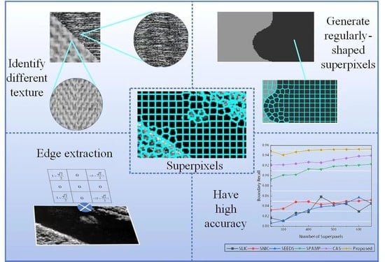
Graphical Abstract

1. Introduction

Synthetic Aperture Radar (SAR) is an active Earth observation system penetrating the ground and taking high-resolution images [1]. Benefiting from the all-day and all-weather advantages of SAR, users can conduct monitoring and reconnaissance in specific scenarios such as battlefields, mineral exploration [2], and oceans [3,4]. The content in SAR images often contains a variety of targets, and accurate target detection or image segmentation is highly critical. SAR image segmentation is a critical preprocessing step before image interpretation, scene recognition, and object detection, and it has become a research hotspot in remote sensing [5,6]. However, there is a considerable amount of inherent speckle noise in SAR images because of the coherency of SAR [7], and the speckle noise seriously reduces the accuracy of image segmentation. Although standard filtering methods can suppress noise, de-noised images exhibit intensity fluctuations and lose details [8]. Since SAR images often contain more target details and have a higher resolution than optical images [9], taking pixels as processing units is undoubtedly a time-consuming problem. Pixel-based SAR image segmentation techniques are sensitive to noise and have high processing complexity. Therefore, the region fusion based on superpixel has been widely used in SAR image segmentation nowadays. A superpixel is an area that contains a certain number of pixels with the same characteristics [10]. An image can be divided into a specified number or size of small segments, with the same attribute using the superpixel method on an image. As a preprocessing step before region merging, superpixel generation is able to over-segment an image, which makes the pixels inside a superpixel have similar properties. Thus, it preserves image information without destroying the edges of objects [11]. Superpixels can reduce the influence of noise for further SAR image processing [12]. Moreover, superpixels will significantly improve the processing efficiency of SAR images [13]. This simple and quick processing method does not require much equipment and is widely used in large scene images such as marine SAR images [14,15]. Therefore, many superpixel generation methods have been proposed to preprocess SAR images and have achieved good results in several critical applications, such as change detection [16,17], object detection [18,19], and image segmentation [12,20,21]. In recent years, many superpixel methods have been proposed for natural images. Simple linear iterative clustering (SLIC) [22] is a low-complexity method that only uses the intensities and locations of pixels for clustering. SLIC has been extended to many application scenarios [23,24], and wide varieties have been produced [25,26,27]. Simple non-iterative clustering (SNIC) [28] is a faster superpixel method that does not require iteration and uses less memory. Superpixels extracted via energy-driven sampling (SEEDS) [29] use the color consistency and the number of pixels contained in the region to segment the image. SEEDS is efficient, but the homogeneity within the region is easily affected by the quality of images. Content-adaptive superpixel segmentation (CAS) [30] is also a superpixel method that extracts texture features by a robust texture descriptor, and it integrates multiple features and introduces a cluster-based discriminability measure that automatically adjusts feature weights to segment images adaptively. These methods achieved good results on general color images.
In addition, some superpixel methods for SAR image segmentation have been proposed according to the special properties of SAR images. Huang [31] proposed a local Bayes-based method to generate superpixels using the probability distribution function of pixels in SAR images. Jin et al. [32] applied an edge-aware-based superpixel generation method and only needed one iteration to complete the segmentation. Mel [33] proposes a gray-level co-occurrence matrix-based superpixel method, which uses the energy and contrast of textures as features. Jing et al. [34] proposed an edge detector and used edge penalty and shrink expansion strategies to generate superpixels. Liang et al. [35] defined a new dissimilarity measure using fast pixel clustering for a noise-based application, fast density spatial clustering, and edge penalty. The similarity ratio-based adaptive Mahalanobis distance algorithm (SRAMP) [36] uses Mahalanobis (instead of Euclidian) distance for SAR images.
Although the above methods can achieve superpixel generation for SAR images, there are deficiencies. The main defect is that most superpixel methods only utilize image intensity and location information for segmentation. Due to the limited usage of features, errors inevitably occur when superpixels are generated, such as incorrect edge fitting and texture region mis-segmentation for texture regions. Although some methods consider boundary constraints when generating superpixels [34], edge extraction in the complex background from SAR images is still challenging. Texture features are seldom used in existing superpixel methods. In addition, some methods ignore the shape regularity of superpixels. The messy shape increases the complexity of computing superpixel features and creates problems for further processing tasks. Some researchers tried to add adjustable coefficients to the method to adjust the shape of the superpixels [37,38] to solve this issue. It is inconvenient to set the suitable coefficients and may cause a loss in precision.
To address this concern, we propose a superpixel method for SAR images based on edge detection and texture region selection (EDTRS). Firstly, we utilize eight convolutional kernels with different coordinate templates to fuse the information of the neighborhood around the target pixel. By defining a detection template, the edge value of the pixel is calculated. We divide the image into nine parts and calculate the 2-D entropy in each grid. The pixels of each region are assigned a new edge intensity by processing the 2-D entropy. Secondly, we take the target pixel as the center and judge whether the texture around the target pixel is periodic by the autocorrelation function. Then, the appropriate region for extracting texture features is selected for the target pixel in combination with the detected edges. The gray level co-occurrence matrix is used to extract the texture of the selected region, and the dimension of the extracted multi-dimensional features is reduced by PCA. Finally, superpixels are generated by K-means clustering using texture features, grayscale differences, and spatial distances.
Compared with other superpixel algorithms, our main contributions and advantages are shown as follows:
(1)
A new edge detection method is proposed, which based on 2-D entropy to eliminate the effect of noise. Using virtual points fused with region information, the resultant edges of the proposed method form a band-shaped area, which meets the requirements of generating superpixels in the later stage.
(2)
A region selection method is proposed, which combines the periodic judgment and edge constraint to select regions for texture feature extraction. The selected region can accurately describe the texture of the target pixel for generating superpixels.
(3)
A superpixel generation method is proposed, which combines edge penalty and texture information. The generated superpixels always retain a regular shape and high accuracy.
The remaining part is mainly constructed as follows: Section 2 elaborates the details of the proposed methods, which contains edge detection, texture region selection, and superpixel generation. Section 3 shows and analyzes the results. Section 4 concludes the main findings.

2. Background and Related Works

The simple linear iterative clustering (SLIC) method was proposed by Radhakrishna [22], where every pixel in the image is assigned to the nearest cluster center by K-means clustering. The initial cluster centers are distributed near each grid’s geometric center, and the grid’s size is set artificially. The integrated distance between the pixel and the cluster center is as follows:
D l = ( d f m ) 2 + ( d s S ) 2
where d f and d s represent the intensity proximity and spatiality proximity between the pixel to be clustered and the center pixel, respectively. m and S are the parameters that weigh the relative contributions of d f and d s to the D l .
The standard SLIC method can accurately segment natural images and has attracted many researchers [23], but it does not satisfactorily process SAR images, especially for trap regions. As shown in Figure 1, Region A and B belong to one class, while the pixel intensities of B and C are closer. We define Region B as a trap region. Since only intensity features and location information are used, SLIC assigns some pixels in Region A and C to a superpixel, resulting in an incorrect segmentation. Taking texture features into account can reduce such errors.
However, there are three issues that need to be given attention when extracting the texture features of pixels: (a) The unit for texture extraction is a region rather than a single pixel [39], (b) texture features at different scales are distinct, and (c) speckle noise in SAR images can be mistaken for texture. Many texture extraction methods have been proposed, such as the Markov Random Field (MRF). These methods have been proven to describe the global texture, but they cannot overcome the above three issues to extract the texture feature of a single pixel.
In the SLIC method, the precision and compactness of superpixels can be adjusted by controlling m and S . In some studies, compactness must be sacrificed to improve superpixel accuracy. The compactness and accuracy of superpixels can be balanced in the following way: increase the spatial constraint for the pixels inside the same object and decrease the spatial control for pixels near the edges of different targets during clustering. This requires us to flexibly generate adaptive spatial constraints according to the detected edges, which demands obtaining as many correct edges as possible and avoids false detections. Most edge detectors use pixels in the eight neighborhoods around the central pixel as targets, ignoring the influence of noise [40]. Some edge detection methods are also easily deceived by gradient changes. In other words, these methods may mistake the texture as a boundary when there is texture inside the target, thus leading to the wrong segments.
Therefore, we use a texture region selection method combined with the fourth-order moment to obtain the texture features of the pixels accurately. We also fuse the non-local information of pixels to eliminate the influence of noise on the edge detector. The extracted edge information is brought into clustering as a spatial constraint to generate accurate and regularly shaped superpixels.

3. Methods

In this section, we explain the proposed method in detail. We first obtain an edge image with a new edge extraction method and 2-D entropy. We use the texture region selection method to extract the texture feature of every pixel. In the final clustering, texture features are used for distance calculation with spatial features and intensity features, and the edge image is transformed into adaptive spatial constraints to control clustering. The flow chart of our method is shown in Figure 2.

3.1. Edge Detection Method

When generating superpixels, we hope the pixels near the target edge have less weight on spatial distances, and more texture and gray features should be considered to improve segmentation accuracy. Therefore, we propose a method to extract the edge of the SAR image. In SAR image edge extraction, we hope that the extracted edge is as close to the actual border as possible. In other words, the extracting edge should contain as many actual borders as possible to reduce the number of wrong edges caused by texture and noise. A Gaussian filter can reduce the influence of noise on edge detection. However, each pixel contains 8 connected neighborhood information, which leads to gradient reduction and edge blurring. Therefore, we redefined the edge detection region before calculating the first derivative of the region.

3.1.1. Generate Virtual Pixel Values

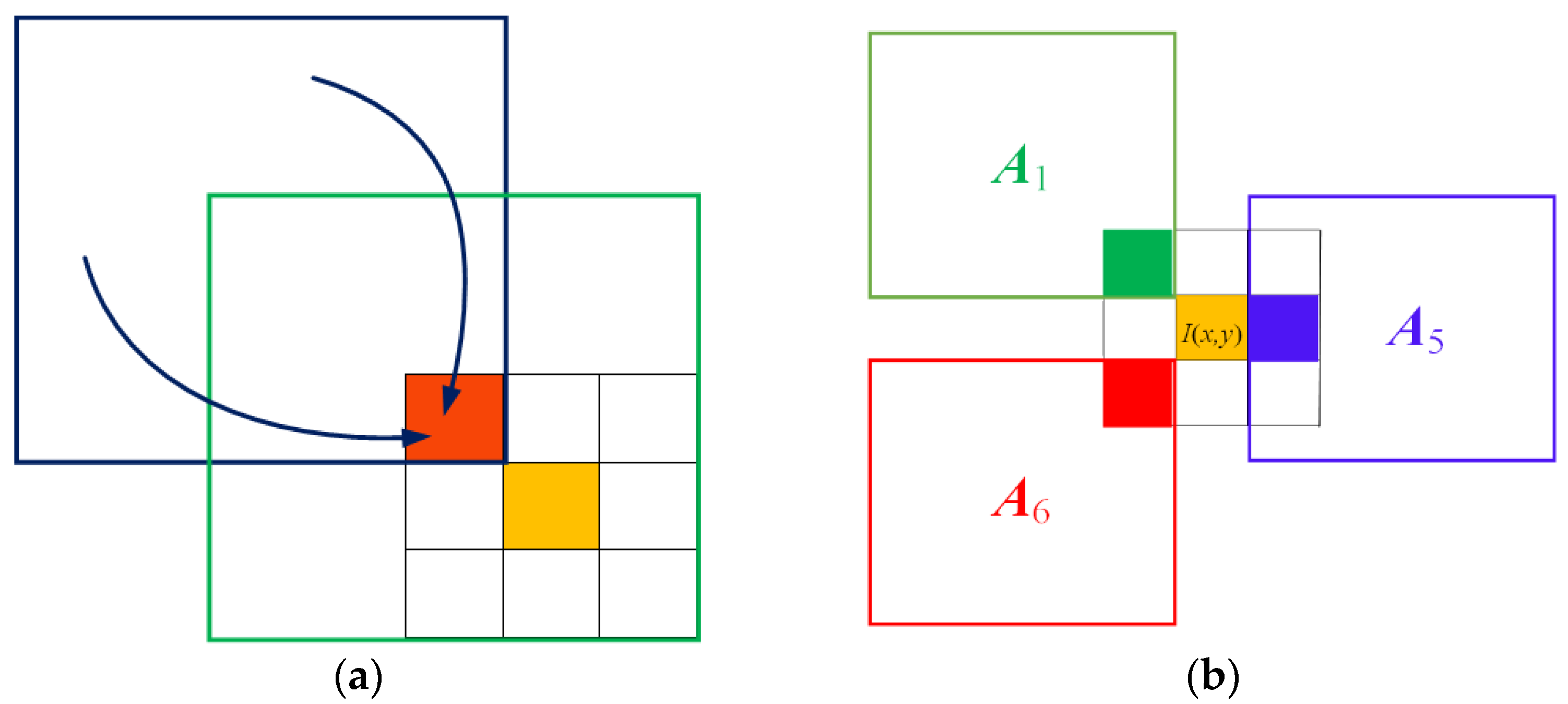
We use the region instead of point to describe the neighborhood information of the target pixel, which can reduce the influence of texture and noise. As shown in Figure 3a, each black grid box represents a pixel, and green and purple boxes represent Gaussian templates at different positions. In traditional Gaussian filtering, a blurred information difference between adjacent pixels in the region to be detected is present. The method we designed is to give the information in the purple box to the pixel where the red rectangle is located to avoid detecting the averaging of the pixel intensity in the region. In each region to be edge detected, its eight-connected neighborhood pixels are redefined, as shown in Figure 3b. I ( x , y ) is a target pixel in image I , and its neighborhood with the size of 11 × 11 is selected to calculate the edge intensity of I ( x , y ) . We take I ( x , y ) as the center and divide its neighborhood area into eight parts A i ( i = 1 , 2 , 3 , 4 , 5 , 6 , 7 , 8 ) from left to right and top to bottom, and each part contains 5 × 5 pixels. The farther a pixel is from the target pixel, the fewer the relationships between the pixel and I ( x , y ) . Therefore, errors will occur when directly summing the intensities of all pixels in this neighborhood area. We use a Gaussian filter to convolute each area so that the eight areas can be replaced by eight virtual pixel values.
However, different from the previous Gaussian filter, we redefine the coordinate template of the Gaussian filter. As shown in Figure 3, the coordinates of the position closest to the target pixel are set to (0, 0) in each region. This new coordinate template uses a two-dimensional Gaussian function to generate a Gaussian filter G i for each part A i , and the calculation formula of G i is defined as follows:
G i ( r , t ) = 1 2 π σ i 2 exp ( r 2 + t 2 2 σ i 2 )
where ( r , t ) denotes the coordinates. The value of σ in the Gaussian function controls how much the weights are spread out. When σ is greater than 2, the value of the Gaussian filter is more evenly dispersed. The farther away it is from the center pixel, the less weight is obtained, and the more independent the final output value is from the pixel value at that distant position. Otherwise, the absolute output value will be the same as the direct summation. In this work, we need to make the value of the virtual point contain distant information but not let the distant pixels have the same weight as the close pixels. When the value of σ is less than 1, the pixels farther from the origin have negligible weights, and the final value is only related to the pixels at the origin. When the homogeneity of the pixels in the region A i is poor, σ i should be small, and the pixels close to the region to be detected have a higher weight. The formula for σ i is as follows:
σ i = 1 10 * var ( A i )
where var ( A i ) represents the variance in the gray values of all elements in A i . Each area is convoluted with its corresponding Gaussian filter to form a new virtual pixel. The calculation of the virtual pixel point i is as follows.
p o i n t i = G i A i
Finally, the eight connected neighborhood pixels in the target region to be detected are replaced by the generated virtual pixels. The new connected region of I ( x , y ) is shown as follows.
b l o c k = [ p o i n t 1 p o i n t 2 p o i n t 3 p o i n t 4 I ( x , y ) p o i n t 5 p o i n t 6 p o i n t 7 p o i n t 8 ]
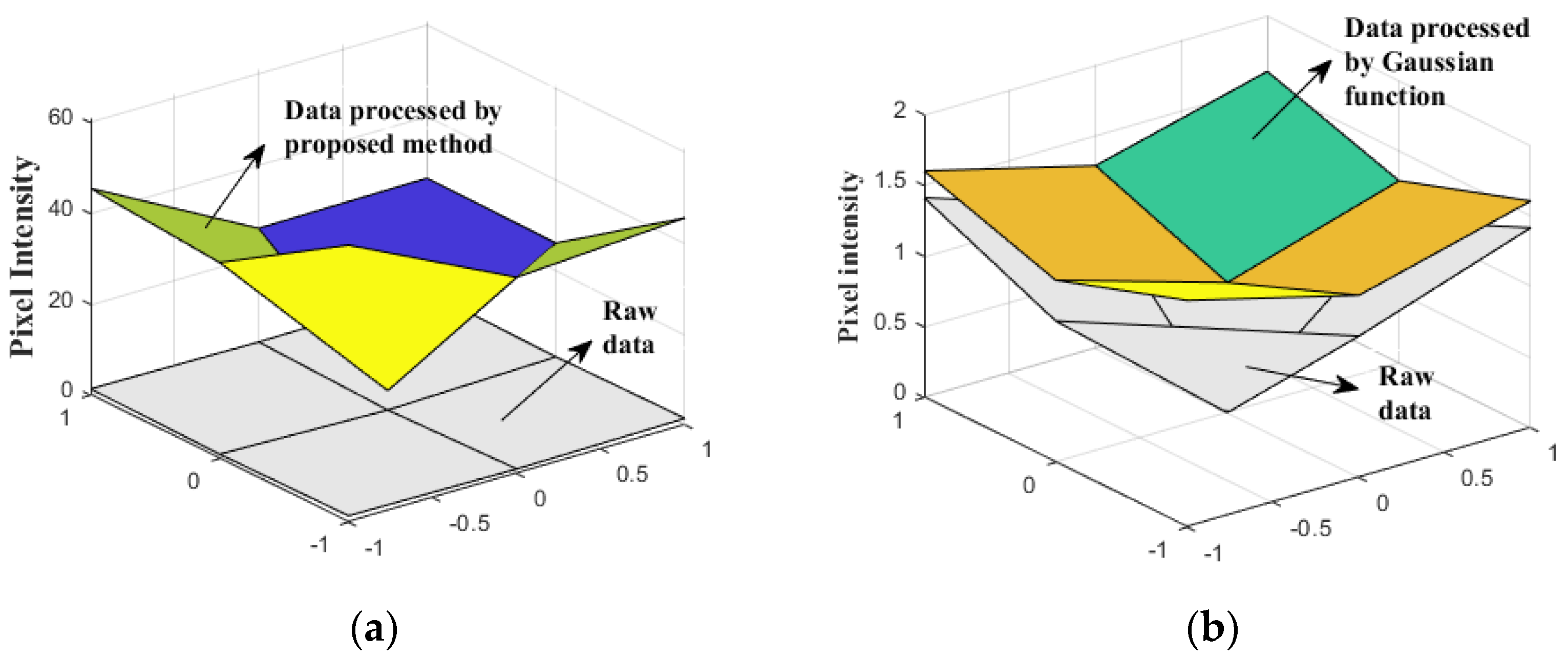
We simulate the intensity of the traditional Gaussian function and the output of our method. As shown in Figure 4, for the target region, the Gaussian function will smooth the intensity and reduce the gradient, while our method can make the gradient more intense.

3.1.2. Using 2-D Entropy to Optimize Edge Values of Pixels

We use a Sobel operator to detect the edge of b l o c k of each pixel to obtain the edge intensity e ( x , y ) of each pixel.
Choosing an appropriate threshold is a critical step in many edge detection methods, and in this study, edge accuracy affects the efficiency and accuracy of the final generation of superpixels. A high threshold will cause actual boundaries to be hidden, while too low a threshold will expose more false boundaries. Yang [41] addressed that the edge percentage of the image has a specific linear relationship with the 2-D entropy of the image and provided edge proportions corresponding to different entropy values. However, SAR images do not have the bright contrasting content of optical images. SAR images also do not have as much edge detail as optical images. For SAR images, the entropy value of some regions exceeds that of others. This high entropy region contains a disordered target instead of many boundaries, as shown in Figure 5. Therefore, where the entropy value is too high, we should reduce the scale of the edge of this region. In the area with a low entropy value, we should enhance the contrast of this region to obtain the actual boundary. However, instead of directly increasing or decreasing the number of boundary pixels by the threshold in an area, we nonlinearly enlarge or reduce the boundary value of the area.
We divide the image into nine areas equally and calculate the 2-D entropy value E N g r i d ( g r i d = 1 , 2 , , 9 ) of each area by [41]. The boundary values of the pixels in each grid are multiplied by their corresponding gain values to form new boundary values.
e n ( x , y ) = e ( x , y ) K ( x , y ) E N g r i d *
Here, the m e a n ( E N ) is the average entropy of the 9 grids in a SAR image, and the K g r i d * is the enlargement and reduction ratio of the boundary score in each grid according to the entropy value. The ratio K g r i d * is defined as follows.
K g r i d * = arctan ( E N g r i d m e a n ( E N ) 10 ) + 2
In Section 3.3, we set 89% of the maximum edge value as the threshold to generate edge images.

3.2. Texture Feature Extraction Based on Region Selection

Only relying on the intensity of pixels to cluster can distinguish objects with significant differences in the gray level, but this method cannot easily distinguish objects with similar gray levels but different textures. Therefore, it is necessary to compute the texture features of each pixel. Since the texture is periodic in the image plane, one period of the texture should be contained in the image area when we extract the corresponding texture feature. We compose the pixel intensities in a specific direction into a sequence, and if the texture is not periodic, we consider that the two sides of the gradient extreme points of the sequence belong to different objects. The procedure of the extraction texture feature is presented as follows.
We take the target pixel ( x , y ) as the center and construct two sequences with the length of L + 1 along its horizontal and vertical directions, respectively.
a v = { I ( x L 2 , y ) I ( x , y ) I ( x + L 2 , y ) }
a h = { I ( x , y L 2 ) I ( x , y ) I ( x , y + L 2 ) }
Outlier detection is used to check the noise to suppress the influence of noise points in SAR images. We use the Local Outlier Factor (LOF) [42] to calculate the local outlier factor for all elements in a v or a h . The formula for calculating the factor L O F L ( r ) of the element in a v or a h is as follows:
L O F L ( r ) = O N L ( r ) l r d ( O ) | N L ( r ) | l r d ( r )
where N L ( r ) is a range. The value of the element in a v or a h is a ( r ) , the distance of a ( r ) and the L th element closest to a ( r ) is N L ( r ) represents [ a ( r ) d L ( r ) , a ( r ) + d L ( r ) ] . l r d ( O ) and l r d ( r ) are the local reachability density of the elements satisfying O N L ( r ) and a ( r ) , respectively.
When the LOF coefficient of the R th element in a is greater than 1, we consider it an outlier, meaning that it is a noise point. Because all elements in this set are continuous in the SAR image, we reassign a ( R ) using mean interpolation.
a ( R ) = a ( R 1 ) + a ( R + 1 ) 2
We regard the processed sequence as a sequence of sequential signals and introduce an autocorrelation function to analyze it.
R ( τ ) = 1 L + 1 a ( r ) a ( r τ )
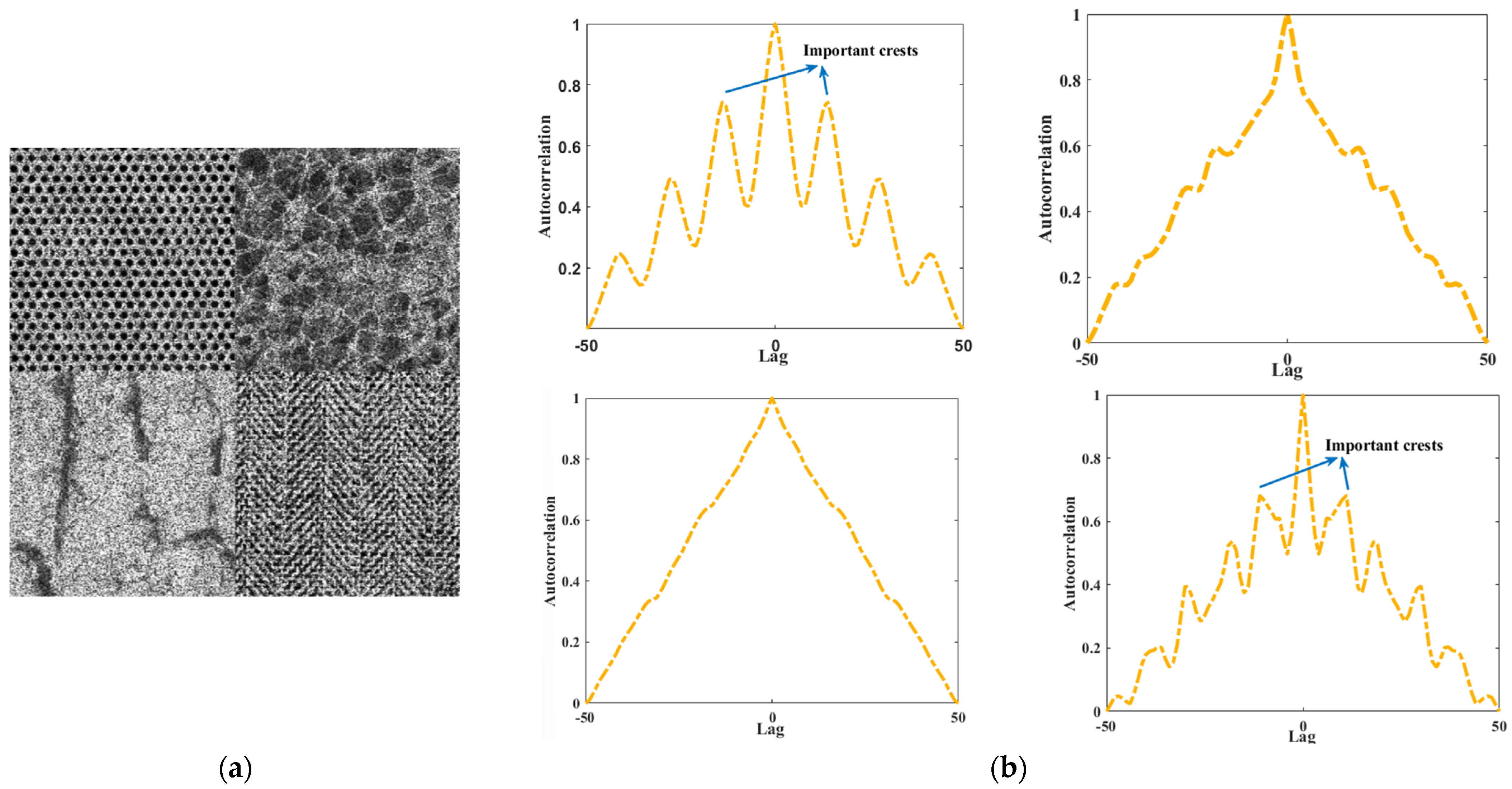
The autocorrelation function R ( τ ) of sequence a has a large crest when τ x ( τ x 0 ) , which means that the sequence probability is periodic and the period is τ x . We synthesize an image containing periodic and aperiodic regions and add a lot of speckle noise. The autocorrelation functions of different regions are shown in Figure 6. The autocorrelation function image of the aperiodic region has no obvious wave crest outside τ = 0 , while the autocorrelation function image of the periodic region has an important wave crest, and the abscissa corresponding to the wave crest represents the period of the texture in the region. In sequence a v and a h , we define the abscissa of the important wave crest as τ a and τ b , respectively. The four vertices of the texture region T R are set to the following: ( x τ a 2 , y τ b 2 ) , ( x + τ a 2 , y τ b 2 ) , ( x τ a 2 , y + τ b 2 ) , and ( x + τ a 2 , y + τ b 2 ) .
When the sequence is nonperiodic, the T R is a fixed area centered on ( x , y ) . However, when the detected edge appears inside the texture area, the detected edge acts as the edge of the T R . We place the T R of each pixel into a rectangular patch with a fixed area to decrease the effect of area size on texture feature extractions.
The grayscale co-occurrence matrix (GLCM) is an excellent texture feature extractor for SAR images segmentation [43]. It shows significant effectiveness in selecting appropriate features due to second-order statistical parameters. We extracted the entropy, energy, contrast, and homogeneity of all regions using GLCM in four directions for a total of 16 features. As shown in Figure 7, the data are reduced to two dimensions by principal component analysis, and the two main features were recorded as FT = { F T 1 , F T 2 } . The extraction of texture features FT can distinguish pixels with similar intensities but different attributions and improve the accuracy of superpixels.

3.3. Specification for Generating Superpixels Based on the Edge and Texture Features

To account for the accuracy and efficiency of generating superpixels, we combined the features extracted in the above two sections. We proposed a superpixel generation method based on edge detection and texture region selection (EDTRS). The detailed flow of pixel clustering is described as follows.
Firstly, set the number of superpixels to K and then compute e and FT of each pixel by the proposed methods in the above two sections. Divide the image into K square grids with size S × S , select a 3 × 3 region in the center of the grid, and set the pixel with the smallest boundary coefficient as the seed point of the grid. Define the seed point as k ( k [ 1 , K ] ) , where its coordinate is ( x k , y k ) , it has a gray value g k , and the texture feature is FT k .
Secondly, update the labels of pixels and cluster centers. For each cluster center, its search range is 2 S × 2 S , so each pixel is searched by several cluster centers. By calculating the distance between the pixel and these cluster centers, the pixel is assigned to a certain label. For SAR image, the distance D between the pixel j to be classified and the cluster center is defined by the following formula:
D = α d l + d g + d t
where d g = ( g i + g j ) 2 is the distance of the gray value, and d t = ( F T 1 , i F T 1 , j ) 2 + ( F T 2 , i F T 2 , j ) 2 is the texture distance. d l is the normalized spatial distance according to the search radius. Parameter α is a highly influential coefficient that determines the quality of the superpixels. The larger α is, the more compact and organized the superpixels are, but the more serious the wrong segmentation is. Since the wrong segmentation occurs entirely at the edge, α should be different for the target pixel located at the edge and not located at the edge. The edge-dependent coefficient α is defined as follows:
α = { exp ( e j ) e j < n max ( E I ) exp ( e j ) e j n max ( E I )
where e j is the edge coefficient of pixel j , and max ( E I ) is the largest value in the edge image E I . Experimentally, n = 89 % yielded the best robustness. When the pixel is on the edge, the value of α is small, ensuring that the classification here follows its features more than the distances. Conversely, when the pixel is far from the edge, the value of α is large, ensuring that the shape of the superpixels in the same object is regular. Afterwards, after assigning all pixels to the label with the smallest distance, update the cluster centers and repeat the above steps.
The proposed EDTRS considers various situations and reduces clustering errors caused by similar intensities but different textures by adding texture distance. In addition, using the calculation of the edge coefficient, whether the pixel is located at the target boundary is determined. The superpixel can retain a regular shape and fit the boundary well using the parameter.

4. Results

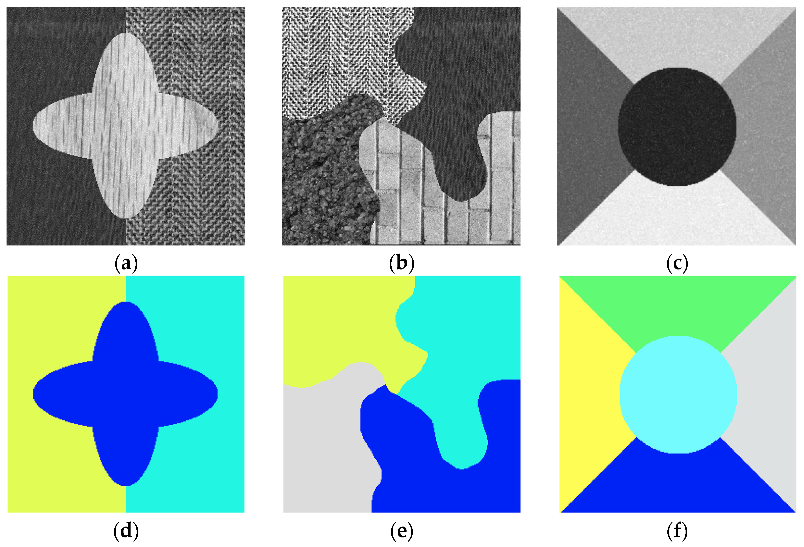
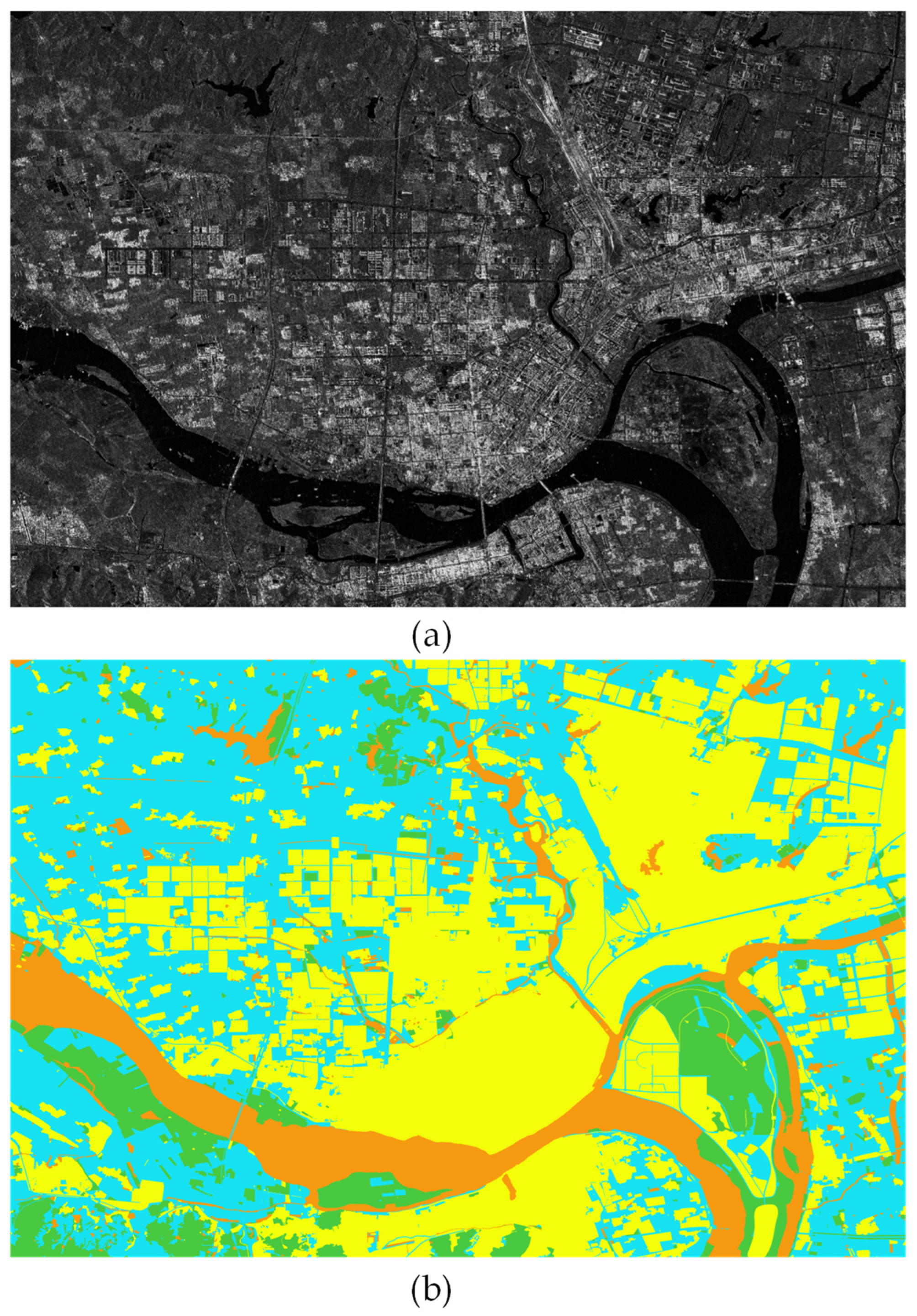
In this section, three simulated SAR images and three real SAR images are used to test the performance of the superpixel algorithm. As shown in Figure 8, the three simulated images S I 1 , S I 2 , and S I 3 ( 512 × 512 ) have three, four, and five types of target images, respectively, and the S I 1 and S I 2 images have textures of different complexities and different average intensities. The S I 3 images do not contain textures. It was proved that using multiplicative Nakagami distribution to add noise to simulate SAR images is effective [44]. We added speckle noise to S I 1 , S I 2 , and S I 3 by using a multiplicative Nakagami distribution model with a variance of 0.1. The first real image S I 4 is Chinalake image with a resolution of 3 m taken by a Ku-band radar. The second real SAR image S I 5 is Piperiver with a resolution of 1 m. Moreover, the third real image S I 6 is from the WHU-OPT-SAR data set, which was taken by the GF-3 satellite. The ground truth that we marked is shown in the Figure 8, Figure 9 and Figure 10. By comparing the segmentation results with the ground truth, the segmentation quality of different algorithms can be objectively evaluated.

4.1. Edge Detection and Texture Region Selection

An excellent edge extraction method is required to extract most of the natural boundaries and should extract a few false boundaries. Therefore, we use two metrics, boundary recall (BR) and boundary precision (BP), to evaluate edge extraction. Their calculation formulas are as follows:
B P = T P T P + F P
B R = T P T P + F N
where T P represents the number of pixels in the detected edge that are true edges, F P represents the number of pixels in the detected edges that are not actual edges, and F N represents the number of true edges that are not detected.
We use four edge detection algorithms as comparison algorithms, namely the Sobel operator, the Log operator, saliency-driven region edge-based top-down level set evolution segmentation (SDREL) [45], and fuzzy logic [46]. The edge extraction method proposed in this paper can obtain the edge value of each pixel, and we use n = 89% as indicated in Section 3.3 as the threshold to generate a binarized edge image. To test the reliability of our proposed edge extraction method, we conduct edge extraction experiments on S I 1 , S I 3 , S I 4 , and S I 5 .
We performed edge detection on four SAR images, which contain high amounts of noise and texture, which is a tremendous challenge for edge detection algorithms. As shown in Figure 11, the edge detection results were obtained from the four contrasting algorithms and the proposed algorithm on four SAR images. Due to the intense noise and texture of the image, the four algorithms were affected to different degrees. The algorithm presented in this paper outperforms all of them. For S I 1 and S I 4 , all four contrast algorithms detected many false edges in strongly textured regions. In contrast, the proposed method effectively alleviated this. For image S I 3 with only noise and no texture, Sobel and the algorithm in this paper detected the boundary well, but the other three methods were inferior. The four contrast algorithms were weak in overcoming noise and detected too many false boundaries for actual images.
As shown in Figure 12, we also computed the edge extraction scores of these five methods for different images. As shown in Figure 12a, the PR scores of the algorithms in the play are shallow, while the proposed algorithm could maintain a high level. The situation in Figure 12b is the same: the edge detection method we proposed can detect almost all of the edges.
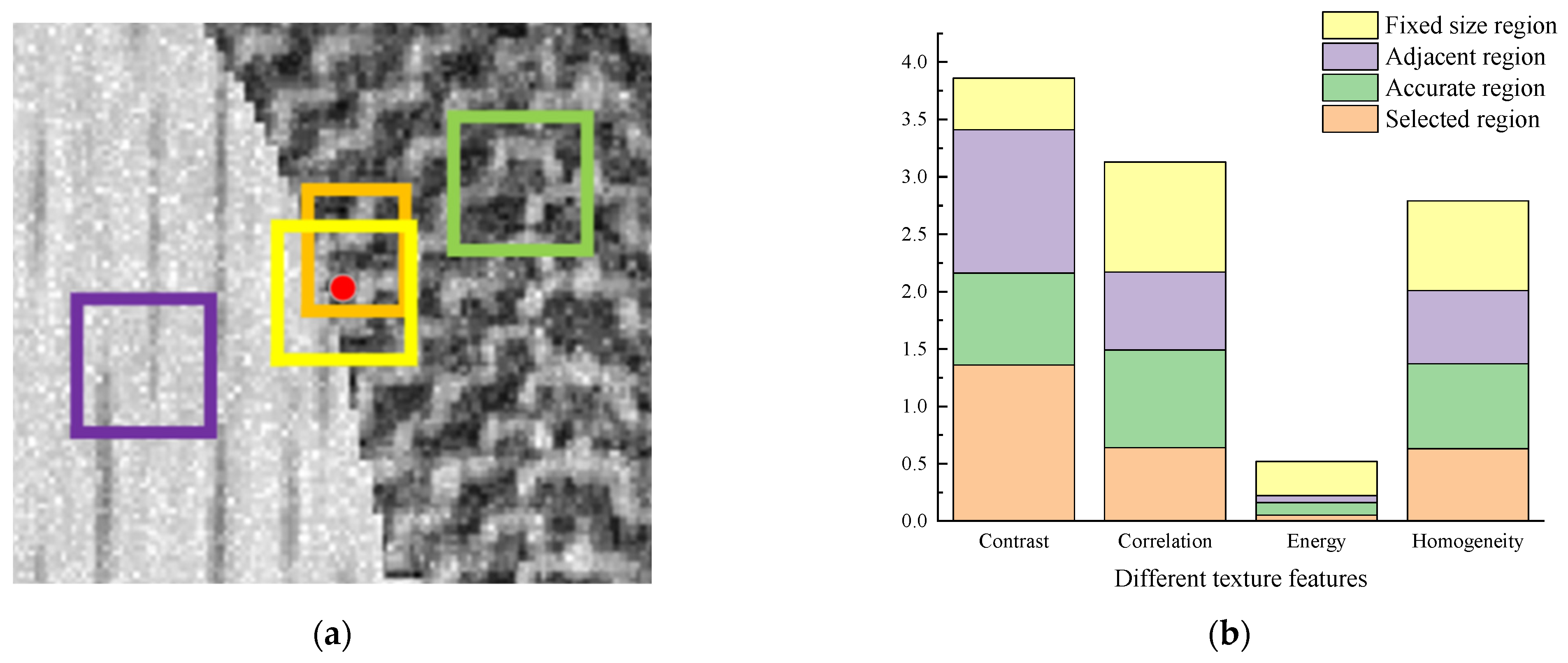
Additionally, we demonstrate the performance of the proposed texture region search method. The texture area search is used to obtain an area that can represent accurate texture information of a given point. Therefore, as long as the texture of this area is consistent, we can consider that the searched area is correct. However, when the explored area contains different surfaces, the method has failed. We used image A as the experimental object and set a target point near the edge, as shown in the red point in Figure 13a. The target point belongs to the same region as the green box. The area for texture feature extraction of the target point in our proposed method is in the orange box, while the fixed size area centered on the target point is in the yellow box. The area inside the yellow box contains two categories of pixels, while the basic and target pixels inside the orange box belong to one category. We use GLCM to extract the texture features of these regions for quantitative analysis. The texture features of the area in the green box in Figure 13a are considered accurate and the texture features extracted from the selected area are very close to the accurate value.

4.2. Superpixel Results

To verify the effectiveness of the proposed algorithm, we compare five representative segmentation algorithms, including SLIC, SNIC, SEEDS, CAS, and SPAMP.
Good superpixel segmentation requires improved boundary adherence, less error segmentation, and a more regular shape. In this study, three commonly used accuracy evaluation metrics are adopted for quantitative comparison: boundary recall (BR), under-segmentation error (UE), and achievable segmentation accuracy (ASA). These three metrics are used to evaluate the precision and accuracy of segmentation. In addition, a metric used to evaluate the shape of superpixels, compactness, and regularity (CR), which is defined as follows:
C R = ( 1 δ 2 i C i 2 4 π ) / ( M × N )
where δ 2 is the variance of all superpixel sizes in an image, C is the perimeter of a superpixel, and ( M × N ) is the area of the image. The larger the C R , the more regular and compact the shape of the superpixel.

4.2.1. Superpixel Results of Simulated SAR Images

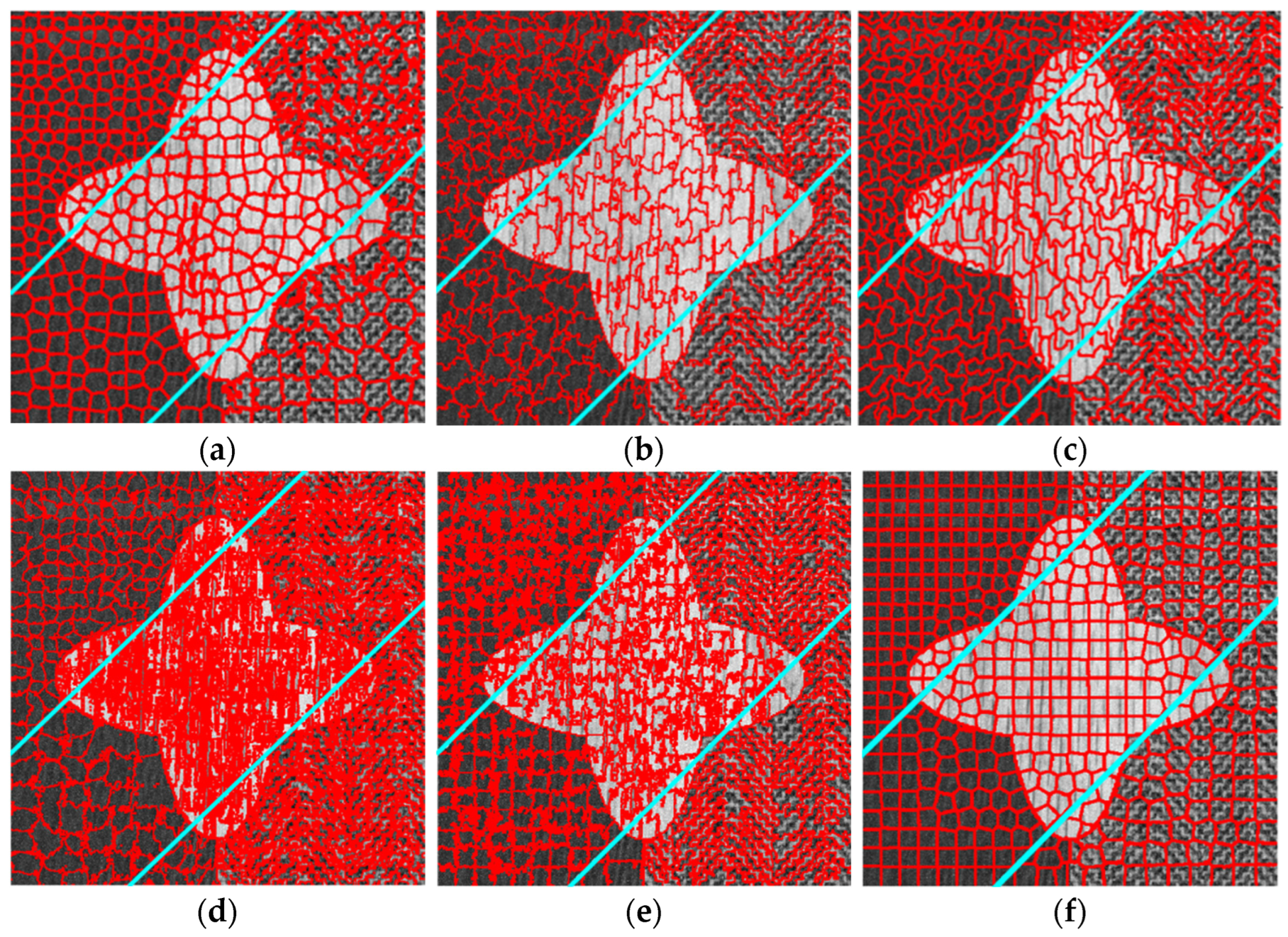
The segmentation results of the six methods on the SAR simulation map containing three types of targets are shown in Figure 14. Each image contains three different numbers of segmentation results, namely 800, 500, or 300 blocks. It can be seen that the superpixel shapes and effects produced by the six methods have their characteristics. The superpixels generated by the SLIC algorithm are more regular in simple textures but perform less well in complex regions. The superpixels generated by the SNIC method do not fit well with the edges, producing many wrong segmentations near the edges. SEEDS divides many pixels with obviously inconsistent intensities into one area, with many wrongly segmented areas. SPAMP and CAS show poor shape consistency in low-textured highlight regions and high-textured regions, but with higher accuracy than the first three algorithms. Compared with the above five algorithms, the performance of the proposed algorithm is superior because the superpixels it generates fit the boundary of the target well and maintain the regularity of the shape in complex textured regions.
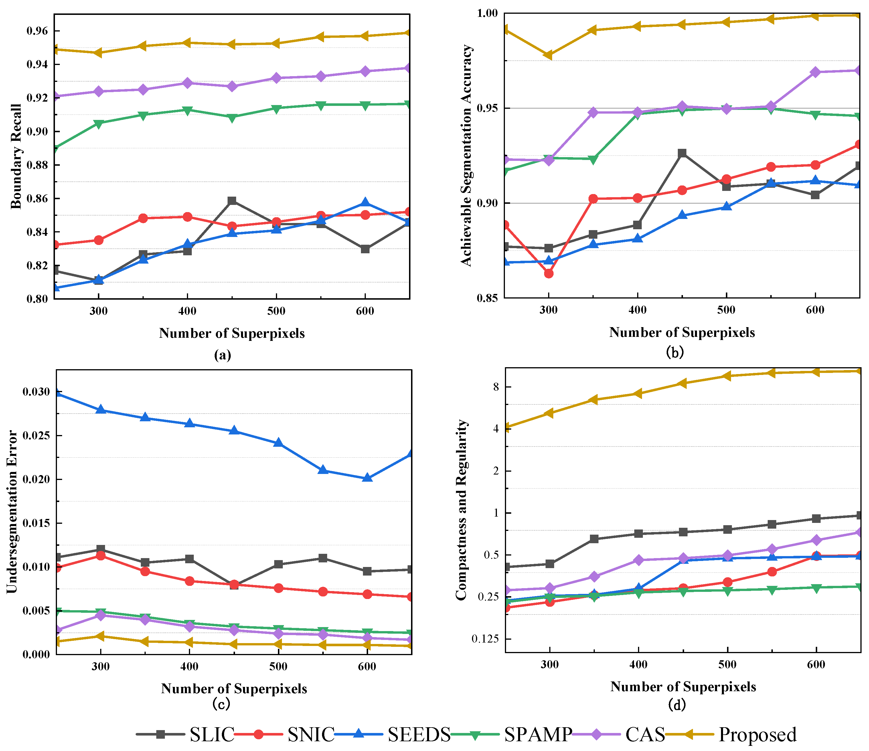
As shown in Figure 15, the evaluation curves represent the six methods with different numbers of superpixels. The performance of superpixels is related to the number of superpixels to a certain extent. The values of ASA and BR rise with the number of superpixels, and the value of UE decreases with the increase in the number of superpixels. When the number of superpixels increases, the pixels in each superpixel decrease, leading to a smaller variance in the number of all superpixels and resulting in a smaller BR value. Therefore, although the BR value can indeed reflect the regularity and compactness of the superpixels, the decrease in the BR value does not necessarily represent a direct relationship between the regularity of the superpixel shape and the number of superpixels. The three indicators of ASA, UE, and BR have shown that the three methods of SLIC, SNIC, and SEEDS generally perform accurately. SPAMP and CAS methods are similar in accuracy and better than the above three methods. The method proposed in this paper achieves the best results in all three metrics. Therefore, our algorithm significantly outperforms other algorithms in terms of shape regularity and compactness.
The S I 2 image has complex textures, and the strongly varying textures make the computer mistake them for edges, which is a massive test for the accuracy of the texture region selection method in the proposed method. Here, we set the number of superpixels as K = 900 , and six methods were used to segment the S I 2 image. The results are shown in Figure 16.
We magnified the regions containing strong textures and the regions containing curved edges to observe the performance of the segmentation results. Regions containing strong textures are interior regions that belong to the same object, although the intensity of the pixels inside this region varies significantly. Combined with Figure 11, the edge detector we proposed does not identify this part as an edge, so the weight of the spatial distance is larger than the distance of other features of the pixels, which enables our method to generate regularly shaped and compact superpixels. In contrast to other methods, since they cannot easily identify real edges, the generated superpixels have chaotic shapes, which are unacceptable to human vision. For the regions containing edges shown in the last row, the superpixel edges generated by our method continuously adhere to the real edges. In contrast, the edges of the superpixels generated by SLIC, SEEDS, and SPAMP are broken with the real edges at several positions, leading to many segmentation errors.
For more clarity, we also calculated the values of the four metrics when the number of superpixels is K = 900 and list them in Table 1.
Both S I 1 and S I 2 are images that contain complex textures. Since the EDTRS has good texture detection characteristics, the segmentation results are excellent. To explore how the algorithm performs in the image without textures, we experiment with images in S I 3 , which do not have texture. We set the number of superpixels to 400, and the segmentation results of the six methods for S I 3 are shown in Figure 17. In the segmentation results of SLIC and SNIC, the target boundary is ignored, and the number of wrong segments is relatively large. In comparison, SEEDS, and the proposed method have almost no inaccurate segmentation and can fit the edge well. Since the images do not contain strong textures, the superpixels produced by the CAS method are regularly shaped and perform better than the first two images.
As shown in Table 2, we calculated the values of four indicators to more accurately verify the reliability of the algorithm proposed in this study.

4.2.2. Superpixel Results of Real SAR Images

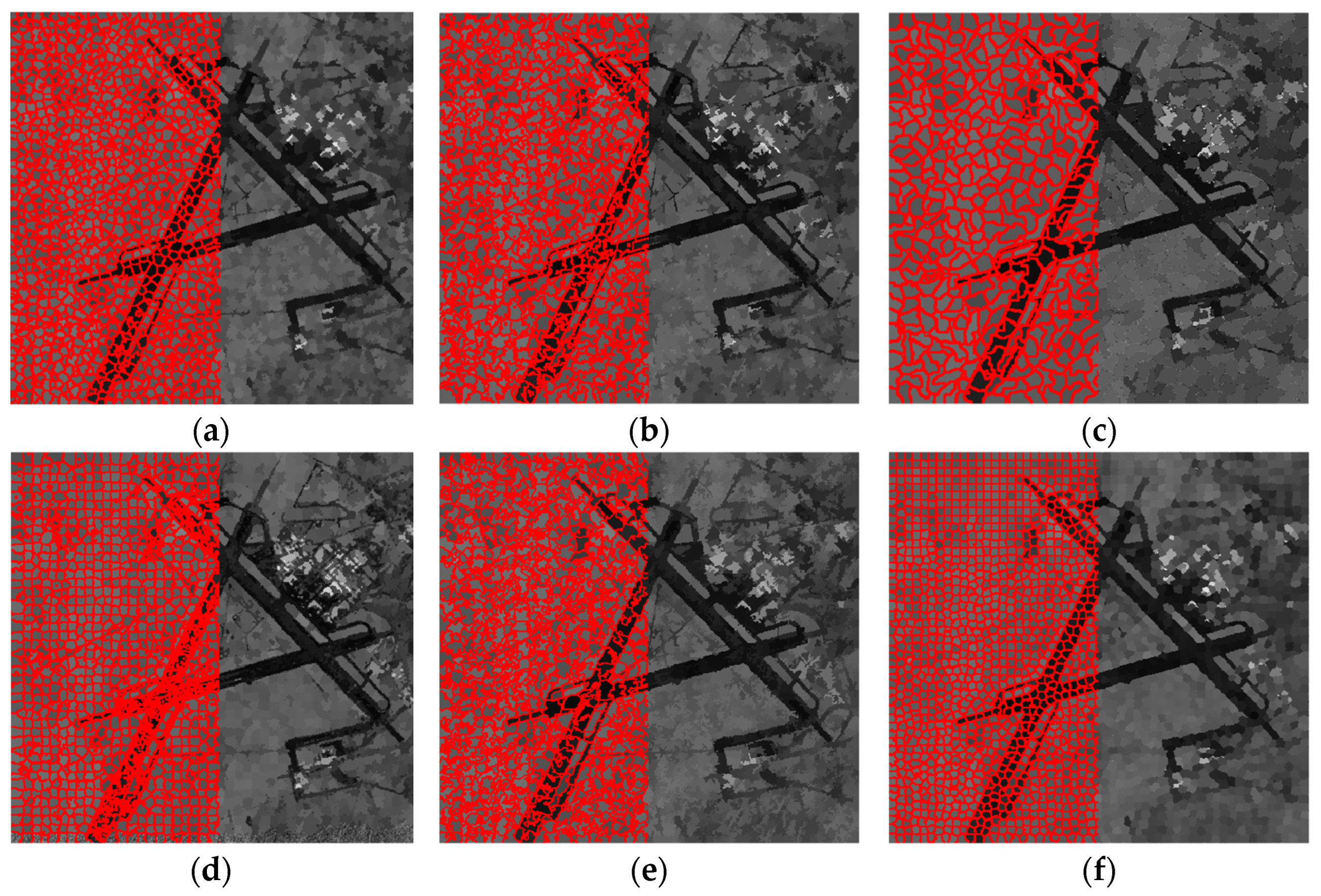
When segmenting the Chinalake image, the number of superpixels was set to 2500. The segmentation results of each method on this image are shown in Figure 18. The average intensity inside each superpixel represents the intensity of the entire image. The superpixel in the left part of the image is surrounded by a red line, which clearly shows the shape of superpixels. In the right part of the image without the red line, the quality of the target boundary segmentation can be distinguished according to the misclassification between regions with different intensities. The results show that the proposed method outperforms the other five in boundary adherence. The superpixels generated by the algorithm in this paper have a regular shape and high compactness. Moreover, the target area with a small area can be well segmented. The superpixels generated by the SLIC, SNIC, and CAS are messy, irregularly shaped, and of varying sizes. Additionally, the segmentation performance of these methods for narrow and long targets is not well satisfactory.
To further compare the superpixel generation results of each algorithm on the Chinalake image, the metrics of each method are shown in Table 3. The superpixels produced by the six methods have curved boundaries and different sizes, but their accuracy is lower than that of the proposed algorithm. The EDTRS algorithm can detect object edges and maintain high shape constraints at non-edges, making the superpixels appear organized and compact overall. At the edge, the clustering of pixels is constrained by adding texture information, which reduces the erroneous segmentation caused when clustering only relies on intensity. Moreover, texture extraction uses the region selection method, which can accurately describe the texture information of pixels. In this way, the algorithm proposed in this paper outperforms the other three algorithms in terms of results.
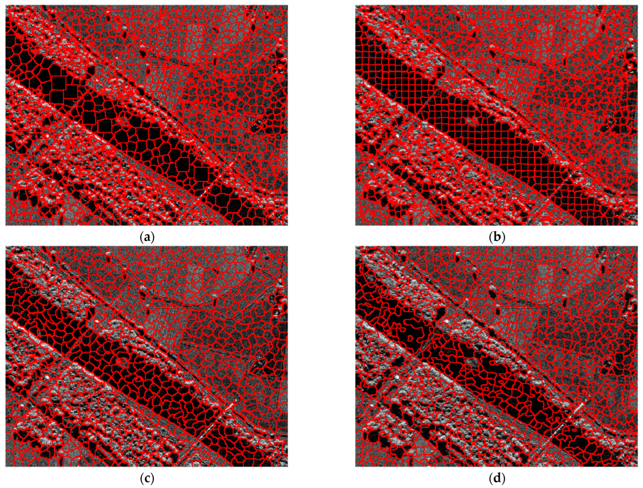
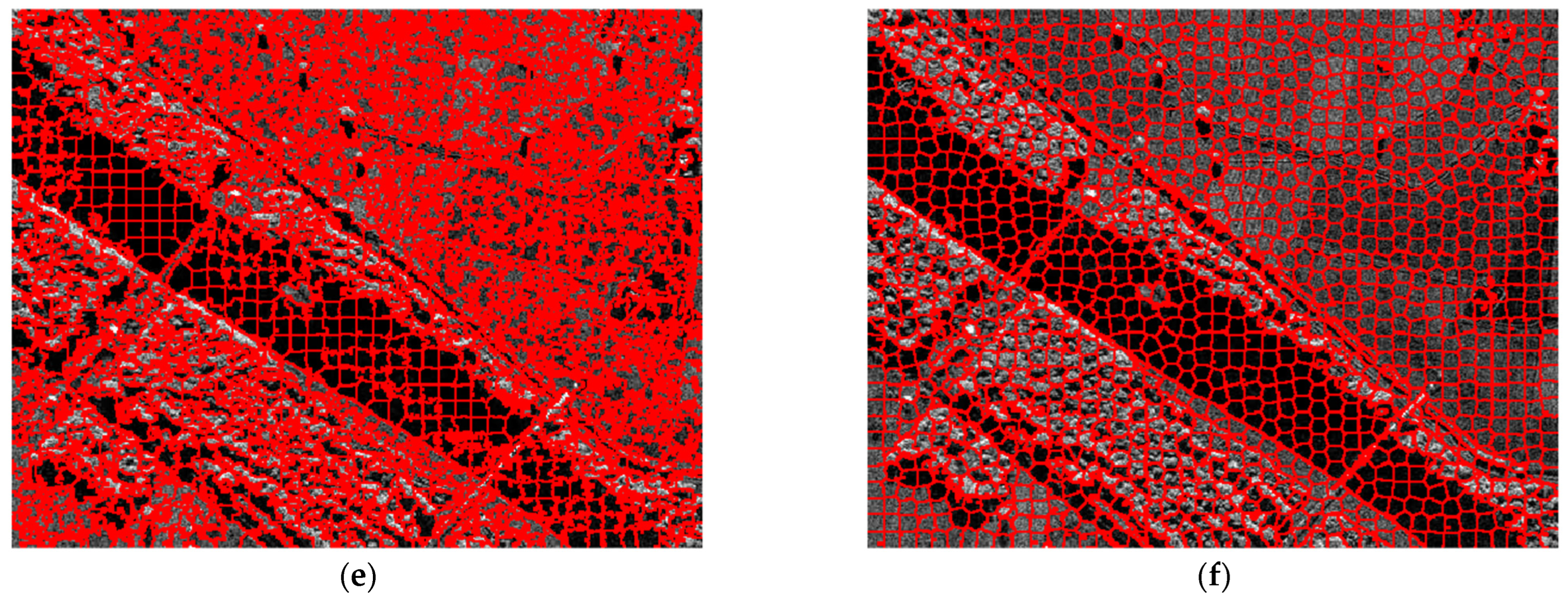
The actual SAR image S I 5 contains more details for its higher resolution compared with Chinalake. Moreover, the background of S I 5 is very complex, containing trees of different sizes and long and narrow bridges. Therefore, it is a massive challenge for the superpixel generation algorithm to overcome the complex texture to generate a regular shape superpixel and to make the edge of the superpixel more consistent with the actual edge. We use six methods to divide S I 5 into superpixels and set the number of superpixels to 1500. The segmentation results are shown in the Figure 19, and almost all methods except SPAMP can fit most of the boundaries. However, seeds and SNIC methods cannot accurately generate superpixels for bridges, and these two methods cannot fully distinguish small and independent trees. On the contrary, the superpixels generated by our method can identify the boundary well and distinguish the small objects in the background. In addition, the superpixels generated by our method are regular in shape and compact.
The third actual image is much larger than the other two and has more noise. The generated superpixels must have good homogeneity to obtain accurate information in the subsequent processing. For S I 6 , the superpixels belonging to buildings should not include the pixels belonging to the land, and the superpixels containing bridges should also avoid pixels belonging to rivers. The more regular the shape, the easier the subsequent extraction of superpixel features. Considering that the original image size is too large, we select a part of the area for display, as shown in Figure 20. Due to the interference of speckle noise, almost all the target edges in S I 6 are not clear, which is a tremendous challenge in generating superpixels. As shown in the blue circle in Figure 20, except for the method in this paper and SEEDS, other methods cannot distinguish the islands in the river well.

4.3. Computation Cost Comparison

Although EDTRS needs to perform boundary detection and texture information extraction before clustering, similarly to SLIC, it only needs to traverse all pixels for clustering to generate satisfactory superpixels. Thus, the time complexity of EDTRS is O ( n ) , where n is the number of pixels in the image.
Table 4 shows the time cost of the six methods of dividing different images into 500 superpixels. All experiments in this paper were performed on a machine with a 2.9 GHz i5 CPU. To obtain the correct texture region, the texture region selection algorithm is used before iterative clustering, and the time consumption of EDTRS also includes the process of obtaining boundary information. Although the proposed algorithm takes longer than other algorithms, the improvement in accuracy and regularity brought by EDTRS makes up for this shortcoming.

5. Discussion

The experimental results of several different edge extraction methods on simulated and real SAR images are shown in Figure 8, showing that most of the edges can be extracted efficiently. Due to solid texture and noise, if the threshold is set too low, too many non-edges will be detected, while if the threshold is set too high, the actual edges will not be extracted completely. Before calculating the edge value of each pixel, our method redefines its eight connected neighborhoods to reduce the influence of noise and texture. Moreover, the edge values of the pixels in the high entropy region are weakened to reduce false edges. Our results show that such a treatment is effective.
In Figure 10, the texture feature of the region selected by our method is closer to the actual texture feature value. However, the edges of objects are curved, leading to some deviations in the extracted features. We will keep focusing on this point in further work. CAS uses texture features to generate superpixels. However, its texture descriptor only focuses on the local information of the target pixel and cannot accurately reflect texture features. Although the accuracy of the superpixels generated by CAS is occasionally higher than other comparison methods, it is lower than the superpixels generated by our method.
In Figure 11, most superpixels can conform to the edges. However, for neighboring regions with similar gray values, the situation becomes worse. In the right half of S I 1 , almost all superpixel generation methods in the intersection of the two regions produce errors. However, the texture features of the two regions are quite different. We can solve the segmentation error caused by the gray similarity by integrating the texture features into the clustering. Figure 12 shows that the greater the number of superpixels, the more significant the relative increase in accuracy. However, when the number of superpixels increases, the number of pixels in a superpixel decreases, and the advantages of superpixels cannot be well reflected. In the blue circle of Figure 15, the superpixels generated by our method are the same in shape and size, but they can still be distinguished when small targets appear. In three real images, the superpixels generated by most methods make fitting the edges well challenging due to the scene’s complexity and noise. Although our methods are also affected, they are generally satisfactory.

6. Conclusions

This study proposes a superpixel generation method based on edge detection and texture region selection. Firstly, we use a Gaussian function to fuse non-location information to generate eight virtual pixels around the target pixel. The edge intensities of all pixels are calculated by convolving the virtual pixels and Sobel operator. Moreover, we use 2-D entropy to assign different edge weights to different regions to reduce the number of wrong edges caused by texture. Secondly, we use the autocorrelation function to analyze the periodicity of the texture and select the region that best represents the texture of the target pixel and calculate the texture features of this region by GLCM. Finally, edge intensities and texture features are combined for pixel clustering.
To evaluate the accuracy of the proposed method, we performed corresponding experiments for three steps of this method. Firstly, we compared our edge detection method with four methods on four SAR images, and the results suggest that our method is superior in terms of accuracy. Secondly, the texture region selection method was tested, and the experimental results directly prove the feasibility of the method. Finally, comparative experiments demonstrate that our proposed method makes excellent progress in segmentation accuracy, boundary adhesion, and superpixel shape regularity. In future work, we will seek to improve the structure of the method to reduce time consumption while maintaining the performance of the results.

Author Contributions

Conceptualization, H.Y. and H.J.; methodology, H.Y., H.J., Z.L., S.Z. and X.Y.; software, H.Y., H.J., Z.L., S.Z. and X.Y.; formal analysis, H.Y. and H.J.; investigation, H.Y. and H.J.; data curation, H.Y., H.J., Z.L., S.Z. and X.Y.; writing—original draft preparation, H.J.; writing—review and editing, H.Y., H.J. and Z.L.; visualization, H.Y.; project administration, H.Y.; funding acquisition, H.Y. All authors have read and agreed to the published version of the manuscript.

Funding

This research was funded by Research Funds for the Central Universities, under Grant (JB211312, XJS221307).

Data Availability Statement

The data presented in this study are available from the corresponding author upon request.

Conflicts of Interest

The authors declare that they have no conflicts of interest.

References

  1. Shang, R.; Peng, P.; Shang, F.; Jiao, L.; Shen, Y.; Stolkin, R. Semantic Segmentation for SAR Image Based on Texture Complexity Analysis and Key Superpixels. Remote Sens. 2020, 12, 2141. [Google Scholar] [CrossRef]
  2. Marghany, M. Advanced Algorithms for Mineral and Hydrocarbon Exploration Using Synthetic Aperture Radar; Elsevier: Amsterdam, The Netherlands, 2021. [Google Scholar]
  3. Marghany, M. Nonlinear Ocean Dynamics: Synthetic Aperture Radar; Elsevier: Amsterdam, The Netherlands, 2021. [Google Scholar]
  4. Shang, R.; Lin, J.; Jiao, L.; Li, Y. SAR Image Segmentation Using Region Smoothing and Label Correction. Remote Sens. 2020, 12, 803. [Google Scholar] [CrossRef] [Green Version]
  5. Li, Y.; Shi, H.; Jiao, L.; Liu, R. Quantum evolutionary clustering algorithm based on watershed applied to SAR image segmentation. Neurocomputing 2012, 87, 90–98. [Google Scholar] [CrossRef]
  6. Fan, S.; Sun, Y.; Shui, P.; Bie, J. Region Merging with Texture Pattern for Segmentation of SAR Images. In Proceedings of the 2019 6th Asia-Pacific Conference on Synthetic Aperture Radar (APSAR), Xiamen, China, 26–29 November 2019; pp. 1–5. [Google Scholar]
  7. Soares, M.D.; Dutra, L.V.; Costa, G.A.O.P.d.; Feitosa, R.Q.; Negri, R.G.; Diaz, P.M.A. A Meta-Methodology for Improving Land Cover and Land Use Classification with SAR Imagery. Remote Sens. 2020, 12, 961. [Google Scholar] [CrossRef] [Green Version]
  8. Gupta, K.; Goyal, N.; Khatter, H. Optimal reduction of noise in image processing using collaborative inpainting filtering with Pillar K-Mean clustering. Imaging Sci. J. 2019, 67, 100–114. [Google Scholar] [CrossRef]
  9. Maged, M. Developing robust model for retrieving sea surface current from RADARSAT-1 SAR satellite data. Int. J. Phys. Sci. 2011, 6, 6630–6637. [Google Scholar]
  10. Chen, Z.; Guo, B.; Li, C.; Liu, H. Review on Superpixel Generation Algorithms Based on Clustering. In Proceedings of the 2020 IEEE 3rd International Conference on Information Systems and Computer Aided Education (ICISCAE), Dalian, China, 27–29 September 2020; pp. 532–537. [Google Scholar]
  11. Qiao, N.; Sun, C.; Sun, J.; Song, C. Superpixel Combining Region Merging for Pancreas Segmentation. In Proceedings of the 2021 36th Youth Academic Annual Conference of Chinese Association of Automation (YAC), Nanchang, China, 28–30 May 2021; pp. 276–281. [Google Scholar]
  12. Xiang, D.; Zhang, F.; Zhang, W.; Tang, T.; Guan, D.; Zhang, L.; Su, Y. Fast pixel-superpixel region merging for SAR image segmentation. IEEE Trans. Geosci. Remote Sens. 2020, 59, 9319–9335. [Google Scholar] [CrossRef]
  13. Ghaffari, R.; Golpardaz, M.; Helfroush, M.S.; Danyali, H. A fast, weighted CRF algorithm based on a two-step superpixel generation for SAR image segmentation. Int. J. Remote Sens. 2020, 41, 3535–3557. [Google Scholar] [CrossRef]
  14. Wang, X.; Li, G.; Plaza, A.; He, Y. Revisiting SLIC: Fast Superpixel Segmentation of Marine SAR Images Using Density Features. IEEE Trans. Geosci. Remote Sens. 2022, 60, 5221818. [Google Scholar] [CrossRef]
  15. Han, L.; Liu, D.; Guan, D. Ship detection in SAR images by saliency analysis of multiscale superpixels. Remote Sens. Lett. 2022, 13, 708–715. [Google Scholar] [CrossRef]
  16. Peng, D.; Yang, W.; Li, H.-C.; Yang, X. Superpixel-Based Urban Change Detection in SAR Images Using Optimal Transport Distance. In Proceedings of the 2019 Joint Urban Remote Sensing Event (JURSE), Vannes, France, 22–24 May 2019; pp. 1–4. [Google Scholar]
  17. Lv, N.; Chen, C.; Qiu, T.; Sangaiah, A.K. Deep learning and superpixel feature extraction based on contractive autoencoder for change detection in SAR images. IEEE Trans. Ind. Inform. 2018, 14, 5530–5538. [Google Scholar] [CrossRef]
  18. Li, T.; Liu, Z.; Ran, L.; Xie, R. Target detection by exploiting superpixel-level statistical dissimilarity for SAR imagery. IEEE Geosci. Remote Sens. Lett. 2018, 15, 562–566. [Google Scholar] [CrossRef]
  19. Du, L.; Li, L.; Wang, Z. A Hierarchical Saliency Based Target Detection Method for High-Resolution Sar Images. In Proceedings of the IGARSS 2019-2019 IEEE International Geoscience and Remote Sensing Symposium, Yokohama, Japan, 28 July–2 August 2019; pp. 13–16. [Google Scholar]
  20. Hou, B.; Zhang, X.; Gong, D.; Wang, S.; Zhang, X.; Jiao, L. Fast graph-based SAR image segmentation via simple superpixels. In Proceedings of the 2017 IEEE International Geoscience and Remote Sensing Symposium (IGARSS), Fort Worth, TX, USA, 23–28 July 2017; pp. 799–802. [Google Scholar]
  21. Yu, H.; Jiang, H.; Liu, Z.; Sun, Y.; Zhou, S.; Gou, Q. SAR Image Segmentation by Merging Multiple Feature Regions. In Proceedings of the 2022 3rd International Conference on Geology, Mapping and Remote Sensing (ICGMRS), Zhoushan, China, 22–24 April 2022; pp. 183–186. [Google Scholar]
  22. Achanta, R.; Shaji, A.; Smith, K.; Lucchi, A.; Fua, P.; Süsstrunk, S. SLIC superpixels compared to state-of-the-art superpixel methods. IEEE Trans. Pattern Anal. Mach. Intell. 2012, 34, 2274–2282. [Google Scholar] [CrossRef] [Green Version]
  23. Boemer, F.; Ratner, E.; Lendasse, A. Parameter-free image segmentation with SLIC. Neurocomputing 2018, 277, 228–236. [Google Scholar] [CrossRef]
  24. Dixit, M.; Pradhan, A. Building Extraction using SLIC from High Resolution Satellite Image. In Proceedings of the 2021 3rd International Conference on Advances in Computing, Communication Control and Networking (ICAC3N), Greater Noida, India, 17–18 December 2021; pp. 443–445. [Google Scholar]
  25. Zhang, L.; Han, C.; Cheng, Y. Improved SLIC superpixel generation algorithm and its application in polarimetric SAR images classification. In Proceedings of the 2017 IEEE International Geoscience and Remote Sensing Symposium (IGARSS), Fort Worth, TX, USA, 23–28 July 2017; pp. 4578–4581. [Google Scholar]
  26. Bai, X.; Cao, Z.; Wang, Y.; Ye, M.; Zhu, L. Image segmentation using modified SLIC and Nyström based spectral clustering. Optik 2014, 125, 4302–4307. [Google Scholar] [CrossRef]
  27. Wu, H.; Wu, Y.; Zhang, S.; Li, P.; Wen, Z. Cartoon image segmentation based on improved SLIC superpixels and adaptive region propagation merging. In Proceedings of the 2016 IEEE International Conference on Signal and Image Processing (ICSIP), Beijing, China, 13–15 August 2016; pp. 277–281. [Google Scholar]
  28. Achanta, R.; Susstrunk, S. Superpixels and polygons using simple non-iterative clustering. In Proceedings of the Proceedings of the IEEE Conference on Computer Vision and Pattern Recognition, Honolulu, HI, USA, 21–26 July 2017; pp. 4651–4660. [Google Scholar]
  29. Bergh, M.V.d.; Boix, X.; Roig, G.; Capitani, B.d.; Gool, L.V. Seeds: Superpixels extracted via energy-driven sampling. In Proceedings of the European Conference on Computer Vision, Florence, Italy, 7–13 October 2012; pp. 13–26. [Google Scholar]
  30. Xiao, X.; Zhou, Y.; Gong, Y.-J. Content-adaptive superpixel segmentation. IEEE Trans. Image Process. 2018, 27, 2883–2896. [Google Scholar] [CrossRef]
  31. Zou, H.; Qin, X.; Kang, H.; Zhou, S.; Ji, K. A PDF-based SLIC superpixel algorithm for SAR images. In Proceedings of the 2016 IEEE International Geoscience and Remote Sensing Symposium (IGARSS), Beijing, China, 10–15 July 2016; pp. 6823–6826. [Google Scholar]
  32. Jing, W.; Jin, T.; Xiang, D. Edge-aware superpixel generation for SAR imagery with one iteration merging. IEEE Geosci. Remote Sens. Lett. 2020, 18, 1600–1604. [Google Scholar] [CrossRef]
  33. Cui, M.; Huang, Y.; Wang, R.; Pei, J.; Huo, W.; Zhang, Y.; Yang, H. A Superpixel Aggregation Method Based on Multi-Direction Gray Level Co-Occurrence Matrix for Sar Image Segmentation. In Proceedings of the 2021 IEEE International Geoscience and Remote Sensing Symposium IGARSS, Brussels, Belgium, 11–16 July 2021; pp. 3487–3490. [Google Scholar]
  34. Jing, W.; Jin, T.; Xiang, D. Content-Sensitive Superpixel Generation for SAR Images with Edge Penalty and Contraction–Expansion Search Strategy. IEEE Trans. Geosci. Remote Sens. 2021, 60, 1–15. [Google Scholar] [CrossRef]
  35. Zhang, L.; Lu, S.; Hu, C.; Xiang, D.; Liu, T.; Su, Y. Superpixel Generation for SAR Imagery Based on Fast DBSCAN Clustering with Edge Penalty. IEEE J. Sel. Top. Appl. Earth Obs. Remote Sens. 2021, 15, 804–819. [Google Scholar] [CrossRef]
  36. Suruliandi, A.; Ramar, K. Local texture patterns-a univariate texture model for classification of images. In Proceedings of the 2008 16th International Conference on Advanced Computing and Communications, Chennai, India, 14–17 December 2008; pp. 32–39. [Google Scholar]
  37. Machairas, V.a. Waterpixels et Leur Application à l′Apprentissage Statistique de la Segmentation. Ph.D. Thesis, Paris Sciences et Lettres (ComUE), Paris, France, 2016. [Google Scholar]
  38. Li, Z.; Chen, J. Superpixel segmentation using linear spectral clustering. In Proceedings of the IEEE Conference on Computer Vision and Pattern Recognition, Boston, MA, USA, 7–12 June 2015; pp. 1356–1363. [Google Scholar]
  39. Akyilmaz, E.; Leloglu, U.M. Similarity ratio based adaptive Mahalanobis distance algorithm to generate SAR superpixels. Can. J. Remote Sens. 2017, 43, 569–581. [Google Scholar] [CrossRef]
  40. Maini, R.; Aggarwal, H. Study and comparison of various image edge detection techniques. Int. J. Image Process. 2009, 3, 1–11. [Google Scholar]
  41. Liu, Y.; Xie, Z.; Liu, H. An adaptive and robust edge detection method based on edge proportion statistics. IEEE Trans. Image Process. 2020, 29, 5206–5215. [Google Scholar] [CrossRef] [PubMed]
  42. Breunig, M.M.; Kriegel, H.-P.; Ng, R.T.; Sander, J. LOF: Identifying density-based local outliers. In Proceedings of the 2000 ACM SIGMOD International Conference on Management of Data, Dallas, TX, USA, 15–18 May 2000; pp. 93–104. [Google Scholar]
  43. Fei, H.; Fan, Z.; Wang, C.; Zhang, N.; Wang, T.; Chen, R.; Bai, T. Cotton classification method at the county scale based on multi-features and Random Forest feature selection algorithm and classifier. Remote Sens. 2022, 14, 829. [Google Scholar] [CrossRef]
  44. Zhu, J.; Wang, F.; You, H. SAR Image Segmentation by Efficient Fuzzy C-Means Framework with Adaptive Generalized Likelihood Ratio Nonlocal Spatial Information Embedded. Remote Sens. 2022, 14, 1621. [Google Scholar] [CrossRef]
  45. Zhi, X.-H.; Shen, H.-B. Saliency driven region-edge-based top down level set evolution reveals the asynchronous focus in image segmentation. Pattern Recognit. 2018, 80, 241–255. [Google Scholar] [CrossRef]
  46. Suryakant, N.K. Edge detection using fuzzy logic in Matlab. Int. J. Adv. Res. Comput. Sci. Softw. Eng. 2012, 2, 38–40. [Google Scholar]
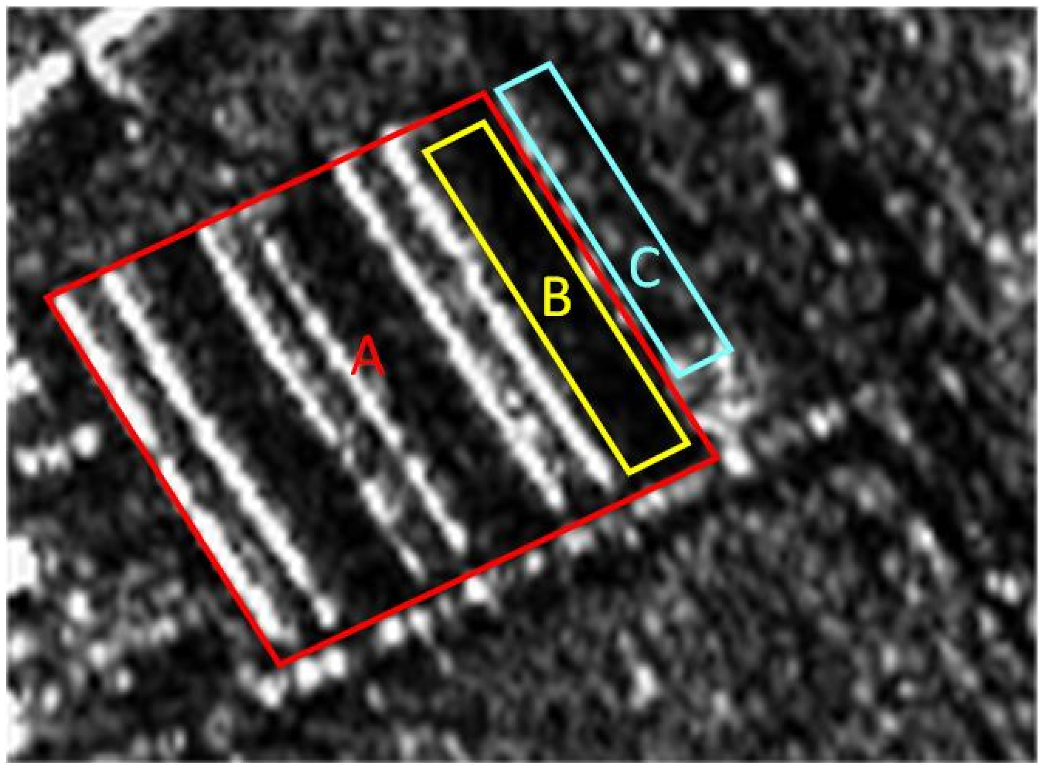
Figure 1. Trap region. Region A and B belong to one class, and Region C is another.
Remotesensing 14 05589 g001
Figure 2. Flowchart for generating superpixels.
Remotesensing 14 05589 g002
Figure 3. The action position of Gaussian function. (a) is difference between the region of our information fusion and the region of Gaussian filtering, (b) is the diagram of generating the redefined pixels.
Remotesensing 14 05589 g003
Figure 4. The schematic diagram of local gradient change. (a) uses Gaussian functions to aggregate information from different directions; (b) filters using Gaussian functions.
Remotesensing 14 05589 g004
Figure 5. Different entropy values for different regions. Both (a) and (b) show the 2-D entropy of scenes with different complexity.
Remotesensing 14 05589 g005
Figure 6. Autocorrelation function graph in different texture states. (a) is a simulated SAR image with four textures, (b) contains four autocorrelation function images of different textures.
Remotesensing 14 05589 g006
Figure 7. Texture feature utilization.
Remotesensing 14 05589 g007
Figure 8. (ac) Simulated SAR images containing three, four, and five types of targets with different textures, respectively. (df) are their corresponding ground truths.
Remotesensing 14 05589 g008
Figure 9. (a) Real SAR image S I 4 ; (b) the ground truth of S I 4 ; (c) real SAR image S I 5 ; (d) the ground truth of S I 5 .
Remotesensing 14 05589 g009aRemotesensing 14 05589 g009b
Figure 10. (a) Real SAR image S I 6 ; (b) the ground truth of S I 6 .
Remotesensing 14 05589 g010
Figure 11. Five edge extraction results for four images. (a) Sobel, (b) Log, (c) SDREL, (d) fuzzy logic, and (e) the proposed method.
Remotesensing 14 05589 g011
Figure 12. Two evaluation metrics for edge extraction. (a) PR metric and (b) BR metric.
Remotesensing 14 05589 g012
Figure 13. (a) Different regions for texture feature extraction and (b) the value of different texture features extracted in different regions.
Remotesensing 14 05589 g013
Figure 14. Superpixel generation results for the image S I 1 . (a) SLIC, (b) SNIC, (c) SEEDS, (d) SPAMP, (e) CAS, and (f) EDTRS.
Remotesensing 14 05589 g014
Figure 15. (a) BR curves for the S I 1 image. (b) UE curves for the S I 1 image. (c) ASA curves for the S I 1 image. (d) CR curves for the S I 1 image.
Remotesensing 14 05589 g015
Figure 16. Superpixel generation results for the image S I 2 . The pictures in the second and third lines show the details in the yellow square in the pictures of the corresponding first line. (a) SLIC, (b) SNIC, (c) SEEDS, (d) SPAMP, (e) CAS, and (f) EDTRS.
Remotesensing 14 05589 g016
Figure 17. Superpixel generation results for the SAR image S I 3 . The edge of the position indicated by the yellow arrow cannot be detected. (a) SLIC, (b) SNIC, (c) SEEDS, (d) SPAMP, (e) CAS, and (f) EDTRS.
Remotesensing 14 05589 g017
Figure 18. Superpixel generation results for the real SAR image S I 4 . (a) SLIC, (b) SNIC, (c) SEEDS, (d) SPAMP, (e) CAS, and (f) EDTRS.
Remotesensing 14 05589 g018
Figure 19. Superpixel generation results for the real SAR image S I 5 . (a) SLIC, (b) SNIC, (c) SEEDS, (d) SPAMP, (e) CAS, and (f) EDTRS.
Remotesensing 14 05589 g019aRemotesensing 14 05589 g019b
Figure 20. Superpixel generation results for the real SAR image S I 6 . (a) SLIC, (b) SNIC, (c) SEEDS, (d) SPAMP, (e) CAS, and (f) EDTRS.
Remotesensing 14 05589 g020
Table 1. Segmentation metrics of S I 2 by four methods.
SLICSNICSEEDSSPAMPCASProposed
ASA0.90150.91870.89100.94090.96380.9789
UE0.22130.24090.25010.21340.20150.1204
BR0.81260.87890.79680.89020.89190.9866
CR1.22530.60420. 45190.31880.40439.9311
Table 2. Segmentation metrics of S I 3 by four methods.
SLICSNICSEEDSSPAMPCASProposed
ASA0.92150.93140.94210.95100.93290.9844
UE0.19110.15760.13010.12090.15960.0993
BR0.90900.95640.96090.97320.95300.9918
CR2.62711.42890.88090.45286.291010.8972
Table 3. Segmentation metrics of the real SAR image by four methods.
SLICSNICSEEDSSPAMPCASProposed
ASA0.90160.92660.94020.92810.93530.95744
UE0.06080.06030.03060.05980.04570.0257
BR0.64740.69160.72680.70190.72400.7987
CR2.06271.02752.11602.67231.234114.32
Table 4. Computation times of four methods in seconds.
SLICSNICSEEDSSPAMPCASEDTRS
Simulated SAR Image
( 512 × 512 )
0.10200.10140.093010.73920.24890.5718
Real SAR image
( 446 × 479 )
0.09840.09560.086710.53270.24030.5450
Publisher’s Note: MDPI stays neutral with regard to jurisdictional claims in published maps and institutional affiliations.