Soil Moisture Prediction from Remote Sensing Images Coupled with Climate, Soil Texture and Topography via Deep Learning

Abstract

Soil moisture (SM) is an important biophysical parameter by which to evaluate water resource potential, especially for agricultural activities under the pressure of global warming. The recent advancements in different types of satellite imagery coupled with deep learning-based frameworks have opened the door for large-scale SM estimation. In this research, high spatial resolution Sentinel-1 (S1) backscatter data and high temporal resolution soil moisture active passive (SMAP) SM data were combined to create short-term SM predictions that can accommodate agricultural activities in the field scale. We created a deep learning model to forecast the daily SM values by using time series of climate and radar satellite data along with the soil type and topographic data. The model was trained with static and dynamic features that influence SM retrieval. Although the topography and soil texture data were taken as stationary, SMAP SM data and Sentinel-1 (S1) backscatter coefficients, including their ratios, and climate data were fed to the model as dynamic features. As a target data to train the model, we used in situ measurements acquired from the International Soil Moisture Network (ISMN). We employed a deep learning framework based on long short-term memory (LSTM) architecture with two hidden layers that have 32 unit sizes and a fully connected layer. The accuracy of the optimized LSTM model was found to be effective for SM prediction with the coefficient of determination ($R^2$) of 0.87, root mean square error (RMSE) of 0.046, unbiased root mean square error (ubRMSE) of 0.045, and mean absolute error (MAE) of 0.033. The model’s performance was also evaluated concerning above-ground biomass, land cover classes, soil texture variations, and climate classes. The model prediction ability was lower in areas with high normalized difference vegetation index (NDVI) values. Moreover, the model can better predict in dry climate areas, such as arid and semi-arid climates, where precipitation is relatively low. The daily prediction of SM values based on microwave remote sensing data and geophysical features was successfully achieved by using an LSTM framework to assist various studies, such as hydrology and agriculture.

1. Introduction

Freshwater resources are being depleted daily due to climate change and the increasing world population. Hence, the effective use of available water is of the utmost importance, which makes its monitoring vital for water savings, mitigation, and adaptation to climate change. In the last decade, soil moisture (SM) monitoring has been investigated with its different aspects, covering drought monitoring [1,2], flood prediction [3], and agricultural applications [4,5]. In particular, in agriculture, SM significantly impacts planning, seeding, fertilization, and irrigation activities. In addition, its close relationship with crop productivity makes SM monitoring an essential factor for optimizing the use of available water resources [6,7].

The dynamics of SM are influenced by the physical properties of topography and soil as well as temporal changes in atmospheric conditions. The impact of these parameters on the variability of SM has been studied in depth concerning topographic data [8,9,10,11], soil texture [11,12,13], and climate variables [14,15,16]. In general, the prediction of SM in local studies (e.g., station-based SM forecasting) does not require static parameters, such as topography and soil texture, because these data vary insignificantly. However, the variability of SM in time depends on climate data in both local, regional, or global scale studies.

In the literature, researchers focused on minimizing the prediction uncertainties to estimate SM by using in situ measurements [17,18,19,20,21]. Including the meteorological parameters in estimating SM enhances the prediction accuracy significantly. The study conducted in [18] predicted the SM values of five stations located in Shandong Province of China by using varying depth measurements of SM together with meteorological variables. A similar study was performed in [19], extending the spatial distribution of stations worldwide, to forecast the SM values. In this study, however, the time series of each station were trained and validated separately. Another study carried out by [20] used the SM values of globally distributed stations of the International Soil Moisture Network (ISMN) coupled with climate, topography, and soil texture data to create a model for the daily prediction of SM in different depth layers. By spatially interpolating SM values of stations to form $0.{25}^{\circ }$ grid cells, the trained model can predict SM in a quasi-global way. Although the sensor measurements provide more reliable estimations of SM values, the dependency of the model on SM sensors limits the use of the model within specific regions where in situ measurements exist. The lack of measurements in high latitudes resulted in poorer forecasts of SM values, specifically in arid regions.

Even though in situ measurements play a crucial role in understanding SM, their spatial coverage and network-related problems make them limited in global studies. Recent developments in satellite-based remote sensing allowed continuous monitoring of the Earth’s surface. In order to overcome the problems encountered in SM predictions when using in situ measurements, satellite data from microwave remote sensing has been used excessively [22,23]. In this context, satellite images are the key to breaking free from the dependency of SM prediction from in situ sensors. The data from the NASA soil moisture active passive (SMAP) [24] and ESA soil moisture and ocean salinity (SMOS) [25] missions are a valuable asset for the global SM monitoring with their 2–3 days temporal resolution. In 2020, ref. [26] expanded the near real-time SM predictions by integrating time series data from SMAP and SMOS missions by using a statistical approach to overcome the inconsistencies between the different SM retrieval algorithms.

Although SMAP and SMOS SM products enable the monitoring of Earth’s surface moisture in high temporal resolution, their applications are constrained due to their coarse spatial resolution. To overcome this limitation, researchers [27,28] used downscaling methods by merging higher-resolution satellite images with lower-resolution SMAP/SMOS data to achieve improved spatial resolution SM predictions. Even though these downscaling efforts are applicable in predicting SM, the generated maps still have an insufficient spatial resolution (∼5.6 km) for applications such as agricultural monitoring. In this regard, the launch of the Sentinel SAR satellites by ESA under the Copernicus Programme paved the way for accurate SM retrieval in smaller scale by acquiring higher spatial resolution microwave remote sensing images [29,30,31,32,33].

SM retrieval from remote sensing images has been improved by the state-of-art machine learning-based regression techniques owing to their ability to learn the relationship between predictors and SM from data [34,35,36,37]. An extensive review on the use of machine learning algorithms for predicting SM can be found in [38]. As computers have improved in performance, deep learning (DL) algorithms have become increasingly popular, as they can handle nonlinear and complex relationships between input and output [39].The SM forecasting studies that use remote sensing images exploited the ability of DL models to capture the spatial and temporal dynamics of SM at the expense of large datasets and high computational costs [5,40,41,42,43,44,45].

Among the different DL methods, artificial neural networks (ANNs) have been proposed to estimate SM from microwave remote sensing images integrated with some auxiliary data [46]. For example, although [47] coupled S1 images with soil texture information, ref. [44] used soil texture and soil temperature data to improve the prediction accuracy of SM retrieval. As an alternative to soil texture data, ref. [48] include climate and topography data to the ANN model. Furthermore, in [42], the combination of soil texture, topography, and climate data was utilized to improve the artificial neural network (ANN) model’s performance.

The recurrent neural network (RNN) is a DL technique that considers the sequential relationships between input data and their effects on the output data. Therefore, such DL models are more appropriate when the sequence modeling tasks are needed, such as SM prediction. However, RNN struggles to learn interdependency between input and output data when the sequence span gets longer [49]. In order to overcome the limitation of this DL technique, a special kind of RNN, long short-term memory (LSTM) is proposed by [50]. With the LSTM, information from a sequence can be carried along the consecutive sequences, and the model can learn the relationship between sequential data and output data.

The study conducted by [51] applied LSTM architecture for the first time in SM studies by using the SMAP L3_SM_P product with climate and soil texture data to improve the design accuracy of SMAP SM data. In 2018, ref. [52] presented a model for the long-term SM forecast on both surface and different depths over the continental US, aiming to exploit the SMAP data together with the land surface models. The model can predict long-term SM values in the same region by using the SMAP SM time series data. In [53], the LSTM model trained with the same data classes used in [51] to nowcast the SM data, when the SMAP L3_SM_P product became available. Another study [54] downscaled the SMAP SM data in (∼1 km) with the help of climate, soil texture, and topography data by implementing LSTM.

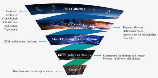
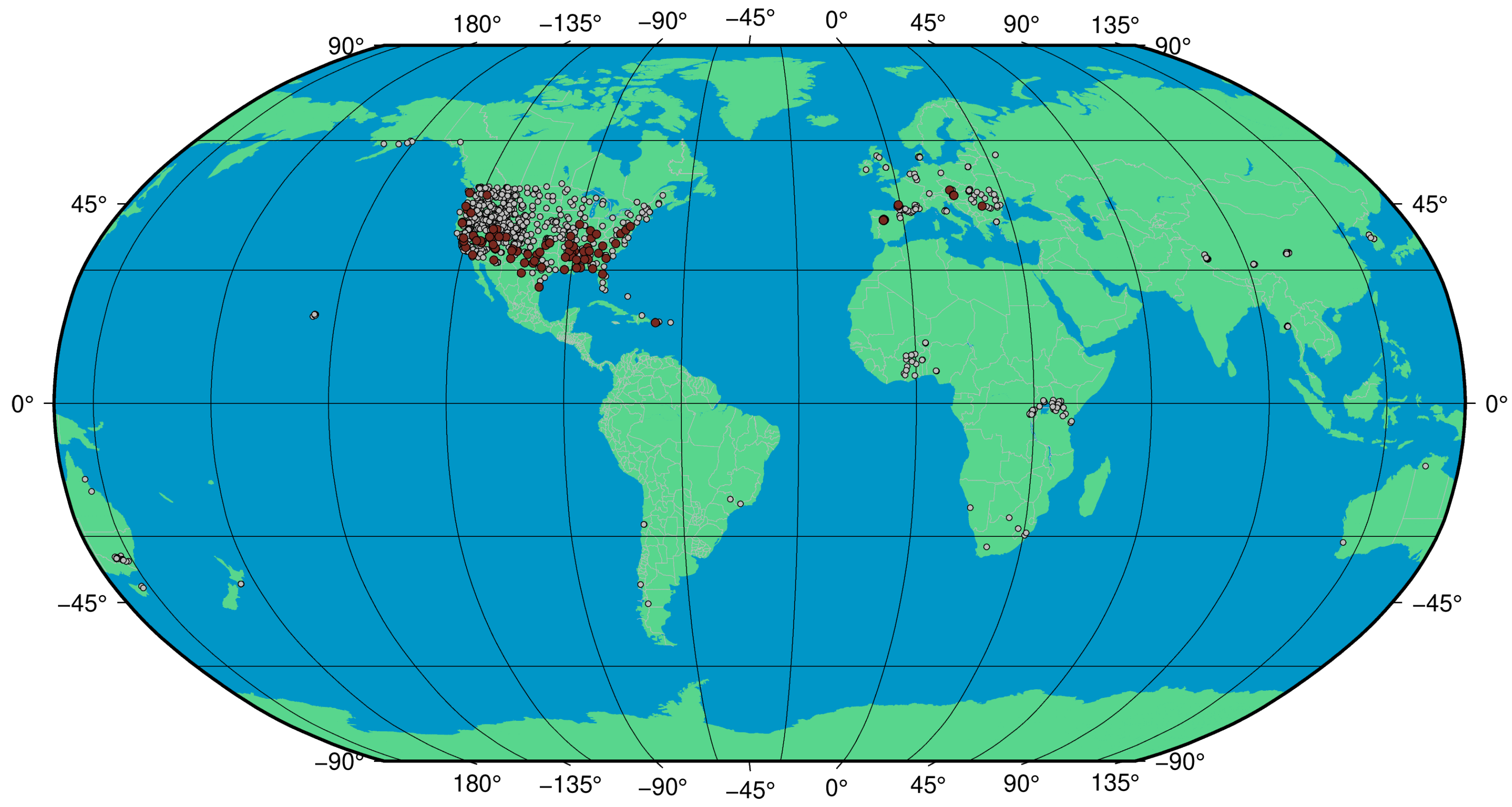
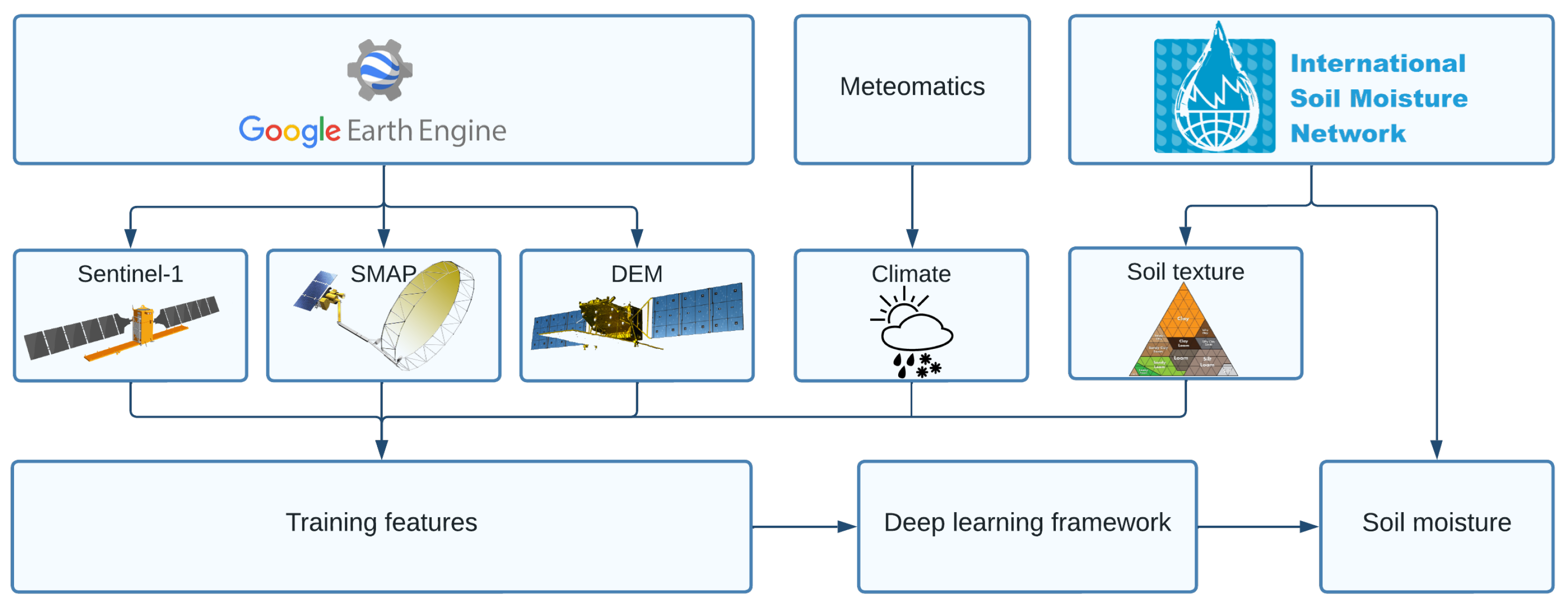
This research aims to improve short-term SM prediction by combining the high temporal resolution SMAP SM product and high spatial resolution S1 backscatter coefficients integrated with the auxiliary data to assist the agricultural activities in the field scale. In this context, we used the SM data of the ground stations from ISMN, distributed around the world, to train an LSTM model with two microwave radar data products (SMAP and S1) together with soil texture, climate, and topographical data that are considered as the predictors of SM. The short-term forecast of SM on a field scale was successfully achieved by utilizing an approach dependent on microwave remote sensing, satellite-based observations. The model used in this study predict accurate SM values of the next day with high spatial resolution in regions with different geophysical properties and climate classes.

The manuscript is structured as follows: Section 2 explains the materials and methods. Section 4 describes the experimental research with data processing, model optimization, and our findings by focusing on the accuracy assessments of utilized methods. Section 5 presents the interpretation of the results and focuses on the effects of land cover, especially in the presence of vegetation, soil texture, and climate, on SM estimation. We finalized the paper by highlighting the important outcomes of this study in Section 6.

2. Materials

In this research, we aim to predict SM by combining the satellite-based data (S1 and SMAP) with soil texture percentages (clay, silt, and sand), topography (elevation, slope, aspect, and hillshade), and climate (temperature, evapotranspiration, and precipitation). By using the features presented in

Table 1. Data used in this research provided with its descriptions, spatial, and temporal resolutions.

Category	Feature Description	Spatial Res.	Temporal Res.
Climate Data 1	T(${}^{\circ }$C), ET (mm) & P (mm)	1 to 5 km	Daily
Satellite Data 2 (S1)	VV, VH & VH/VV	10 m	6–12 days
Satellite Data (SMAP)	Surface & Subsurface SM (mm)	10 km	3 days
Soil Texture	Sand, Clay, Silt (%)	Point-wise	Constant Values
Topographical Data 3	H (m), S (${}^{\circ }$), A (${}^{\circ }$), HS (${}^{\circ }$)	30 m	Constant Values
Soil Moisture Data	SM of top 5 cm (m${}^3$/m${}^3$)	Point-wise	15 min

¹ T: temperature, ET: evapotranspiration, P: precipitation, ² S1 backscatter coefficients in linear scale, ³ H: elevation, S: slope, A: aspect, HS: hillshade.

, we modeled the SM in time by using an LSTM framework. The statistics of these features were presented in

Table 2. The statistics of features used in the study.

Feature	Mean	Std	Feature	Mean	Std
Temperature (T)	8.81	11.03	Sand	42.81	13.91
Evapotranspiration (ET)	2.80	1.96	Clay	18.77	6.90
Precipitation (P)	2.64	11.01	Silt	38.42	10.87
VV	0.019	0.019	Elevation (H)	1400.48	1150.57
VH	0.088	0.076	Slope (S)	7.55	7.16
VH/VV	0.229	0.281	Aspect (A)	162.99	104.83
SMAP SM (Surface)	14.70	8.62	Hillshade (HS)	180.10	23.09
SMAP SM (Subsurface)	52.56	37.97	Soil Moisture (SM)	0.18	0.12

.

2.1. International Soil Moisture Network

ISMN is a data-hosting facility developed and still maintained by several universities [55,56,57]. It is supported by the European Space Agency’s (ESA) Earth Observation program. The ISMN stations include soil texture properties and SM values in time, freely available at https://ismn.geo.tuwien.ac.at/ (accessed on 17 August 2022). When we started the algorithm development, the total number of available stations was 1611 after 2017, when S1 data became available. The locations of the stations cover different climates and ecoregions. However, ∼70% of the available stations were located in the USA (see Figure 1).

In addition to the station locations, in Figure 2, we present the ternary distribution of the soil data. Ternary distribution depicts the data in a 3D space, making it simpler to understand relations. Figure 2 shows that most soil samples are located in the loam class, followed by sandy loam, clay loam, and silty loam.

Along with the soil texture and SM data, the metadata of each station includes land cover based on the ESA CCI land cover product [58] and Köppen–Geiger climate classes [59]. It should be noted that these data were used only for the evaluation of the model performance w.r.t. varying land cover and climate class of the stations, not for training the model.

2.2. Satellite Data

In this research, we accessed all satellite data via the Google Earth Engine (GEE) Python application programming interface (API) [60]. From the GEE, we downloaded the S1 data—one of the missions of ESA’s Copernicus initiative—together with NASA’s SMAP data on the location of the SM stations. Their ensured continuity for the future and sensitivity to changes in vegetation and soil properties makes both satellites a viable option for SM monitoring [5,61,62,63,64].

2.2.1. Sentinel-1 (S1)

S1 is a synthetic aperture radar (SAR) satellite mission with a C-band (5.6 cm) sensor. The advantage of S1 lies in its sensitivity to SM content [65]. There are two identical satellites in the S1 mission, S1a, and S1b. Each satellite has a temporal resolution of 12 days, resulting in an average of a six-day repeat cycle. Unfortunately, in December 2021, S1b failed data dissemination and became space junk. Since then, S1a has been providing data alone, and its temporal resolution depends on the area, with a minimum orbit repeat cycle of six days in Europe and 12 days in other areas. ESA is planning to launch S1c in the first half of 2023 to continue the dual satellite constellation.

This research used the ground range detected (GRD) 10-meter spatial sampled data processed by ESA. The data we have selected has vertical transmission–vertical received (VV) and vertical transmission–horizontal received (VH) polarizations.

In this study, all S1 passes between 31 December 2017 and 1 January 2021 were included for each station of ISMN. In the data processing step, 50 m × 50 m region of interest was defined around each station to calculate the mean value of S1 GRD backscatter signals. The mean backscatter signals were converted from logarithmic scale to linear scale. Additionally, the VH/VV ratio was added as a feature to the dataset.

2.2.2. Sentinel-2 (S2)

S2 is a multi-spectral instrument (MSI) satellite mission with spectral sensitivity to the visible-near-infrared region of the electromagnetic spectrum. In this mission, like S1, there are two identical satellites (a and b). Both satellites have a temporal resolution of 12 days, also resulting in an average of a six-day repeat cycle.

In our research, we used the Level-2a surface reflectance product processed by ESA. The data has 13 bands ranging from 10- to 60-m spatial resolution. We only used red and near-infrared bands to derive the vegetation indices. As in the case of S1, pixels within the 50 m × 50 m region of interest around the stations were extracted to calculate the mean NDVI values. However, this feature was only used to evaluate the model performance in the presence of vegetation and was not included in the feature set to train the model.

2.2.3. Soil Moisture Active Passive (SMAP)

In 2015, NASA launched the SMAP satellite to monitor the SM content by using L-band SAR (active) and radiometer (passive) instruments. SMAP has a temporal resolution of 2–3 days globally. In this research, we used Level-3 data of SMAP SM, which has 10-km spatial resolution [66].

2.2.4. Topography

The topography of the surface also influences the variation in the SM. With the GEE platform, topographic parameters, such as elevation, slope, aspect, and hill shade are obtained from the ALOS DSM Global 30 m dataset [67].

2.3. Climate Data

As an integral part of the water cycle, the dynamics of SM are closely associated with climate data, such as precipitation, temperature, and evapotranspiration. In this research, we gathered the precipitation (P), air temperature (T), and evapotranspiration (ET) data on the location of the SM stations by using the Meteomatics API [68]. The available meteorological data have a spatial resolution ranging from 1 km to 5 km. Under the assumption of lower spatial variability, we used the reported data without changing the processing pipeline. The usage of the API was made possible within the service provided to AgriCircle AG by Meteomatics.

2.4. Data Preprocessing

For SM modeling, we created a dataset that combines static and dynamic features, as previously shown in Table 1. The static features are soil texture and topography; the dynamic features are climate and satellite-derived time-series data. In addition, we added a time variable as a dynamic feature. Because the LSTM framework requires time-series data, we repeated the static features as the sequence length before feeding it to the LSTM framework.

For dynamic features, we prepared a three-year dataset that includes in situ observations acquired from ISMN stations from 31 December 2017 to 1 January 2021. In this dataset, we applied data cleaning to reduce the data-originated uncertainty and eliminate the inconsistency within the measurements. Data cleaning involves a two-step elimination criteria. The first criterion is related to the record length. The record length condition requires that those stations be discarded if more than 10% of the measurements were missing in any station. The second criterion is developed to ensure sequential dependence in the observations. The SM stations with more than 60 consecutive days of missing measurements are also excluded from the analysis because a solution like interpolation was unrealistic considering the complex nature of the problem. According to these criteria, we found 103 stations, shown by red dots in Figure 1, out of 1611 with time series of SM measurements suitable for the analysis. Because dynamic features are gathered from various sources with different temporal resolutions, we upsampled all data into daily sampling by using the linear interpolation method for temporal matching. The ground measurements are resampled into daily SM values to ensure the matching temporal resolution.

For the training of the LSTM model, we formed five different scenarios to determine the contribution of feature groups. As previously shown in Table 1, in SM monitoring, climate data, soil texture, and topographical data are the main drivers of SM. Beginning with the climate data (Case I), we consecutively included soil texture (Case II), topographical data (Case III), and satellite data (Case IV and Case V) and listed them below.

Case-I

Climate data

Case-II

Climate data, soil texture

Case-III

Climate data, soil texture, topographical data

Case-IV

Climate data, soil texture, topographical data, satellite data (SMAP)

Case-V

Climate data, soil texture, topographical data, satellite data (SMAP, S1)

In each case, time variables (sine and cosine of time) are kept within the features set because they are independent variables that represent the positional encoding of input features in a time series.

3. Methods

We employed the satellite data, soil texture, climate, and topography features mentioned above to forecast the SM by using the following process chart shown in Figure 3. The process starts with the first row and ends with the accuracy assessment and prediction of SM.

3.1. Long Short-Term Memory

As a descendent of RNN, [50] proposed an approach called long short-term memory (LSTM) to overcome the vanishing gradient problem in RNN. In LSTM, the ordinary unit cell repeats the input–output sequence; in RNN, this is replaced by a memory cell. LSTM contains three gates: the input gate $i_t$, forget gate $f_t$, and output gate $o_t$. In addition to these gates, there are two different parts: cell state $c_t$, which keeps information from previous states and transfers it to the next, and the hidden state $h_t$, which is the output of the LSTM cell. The equation of input gate, forget gate, and output gate is defined as

$$\begin{array}{cc}\hfill i_t& =\sigma \left(w_i\left[h_{t-1},x_t\right]+b_i\right)\hfill \end{array}$$

(1)

$$\begin{array}{cc}\hfill f_t& =\sigma \left(w_f\left[h_{t-1},x_t\right]+b_f\right)\hfill \end{array}$$

(2)

$$\begin{array}{cc}\hfill o_t& =\sigma \left(w_o\left[h_{t-1},x_t\right]+b_o\right),\hfill \end{array}$$

(3)

where $w_i$, $w_f$, and $w_o$ are the weight matrix, $x_t$ is input, $h_{t-1}$ is the hidden state from previous time step, $b_i$, $b_f$ and $b_o$ are bias vector and $\sigma$ is the sigmoid activation function for the gates. The activation functions introduce nonlinearity by transforming inputs to targeted outputs with a nonlinear regression procedure, making the model capable of learning and performing more complex tasks. After the calculation of gates, the cell state and hidden state can be defined as

$$\begin{array}{c}\hfill c_t=f_t\odot c_{t-1}+i_t\odot \mathit{tanh}\left(w_c\left[h_{t-1},x_t\right]+b_c\right)\end{array}$$

(4)

$$\begin{array}{c}\hfill h_t=o_t\odot \mathit{tanh}\left(c_t\right),\end{array}$$

(5)

where $w_c$ is the weight matrix, $c_{t-1}$ is the cell state from the previous time step, $b_c$ is the bias vector, $tanh$ is the hyperbolic tangent activation function and ⊙ is the element-wise multiplication. The size of the weight matrix is determined according to the unit size and hidden layer size of the LSTM model, feature vector dimension, and feature sequence length. It should be noted here that the weight matrix of LSTM does not change through timesteps. For detailed information please refer to [69].

3.2. Accuracy Assessment

Four accuracy metrics, namely, coefficient of determination ($R^2$), root mean square error (RMSE), unbiased root mean square error (ubRMSE), and mean absolute error (MAE) were used to evaluate the performance of the implemented model for the SM prediction. We have

$$\begin{array}{cc}{R}^2=1-\frac{{\sum }_{i=1}^N{\left(y_i-{\widehat{y}}_i\right)}^2}{{\sum }_{i=1}^N{\left(y_i-{\overline{y}}_i\right)}^2}\hfill & MAE=\frac{{\sum }_{i=1}^N\left|y_i-\widehat{y}\right|}{N}\hfill \\ RMSE=\sqrt{\frac{{\sum }_{i=1}^N{\left(y_i-{\widehat{y}}_i\right)}^2}{N}}\hfill & ubRMSE=\sqrt{{\left(RMSE\right)}^2-{\left(\frac{1}{N}{\sum }_{i=1}^N\left(y_i-{\widehat{y}}_i\right)\right)}^2}.\hfill \end{array}$$

In the above equations, $y_i$, ${\widehat{y}}_i$, and ${\overline{y}}_i$ indicates actual SM, predicted SM, and mean value of the actual SM, at ith time step, respectively. Out of these four metrics, we use $R^2$, RMSE, and ubRMSE to evaluate the performance and MAE for station-based assessments of the trained model.

3.3. Implementation of the LSTM Framework

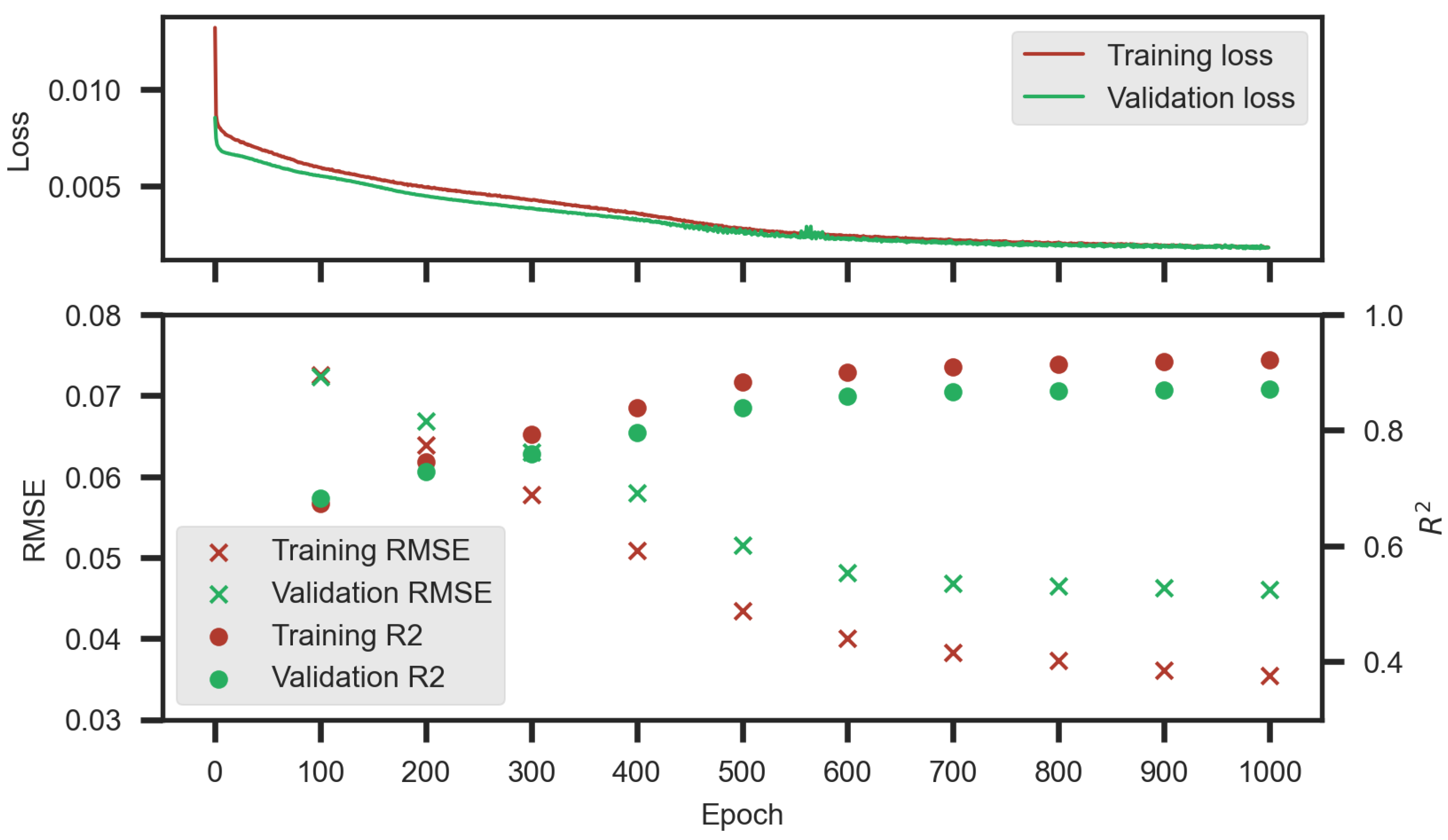
The SM value at time t ($Y_t$) was predicted by using n number of input features with previous w sequential days (window size) as $[X_{t-1}^n\cdots X_{t-w}^n]$. After preparing the dataset, we divided it temporally into 60% for training, 10% for validation, and 30% for testing purposes. The temporal split corresponds to 658 days used to train the model starting from 31 December 2017 until 20 October 2019, 109 days used to validate the model training between 21 October 2019 and 6 February 2020, and 330 days used to evaluate the trained model from 7 February 2020 until 1 January 2021. Whereas the LSTM model was built with training data, the hyperparameter tuning was carried out by using a validation dataset. After the optimum hyperpamater set was determined, independent evaluation of the model was conducted based on testing data.

Before starting the training, we normalized all the input features via the MinMaxScaler function of the sklearn Python package to ensure numerical stability. For the normalization, we followed different strategies for static and dynamic features. By their nature, the static features have global minimum and maximum values; therefore, we normalized them together. On the other hand, dynamic features have local variations that change each station’s minimum and maximum values, leading to a station-based normalization.

One of the primary flexibility features involved in the use of time series data is the varying length of past data to make future predictions. In such a structure, the number of previous timesteps is called the window size. The window size parameter must be selected carefully because it impacts forecast accuracy. For its determination in the SM forecast, we reformed the original dataset according to different window sizes: last one day, five days, ten days, and thirty days.

The LSTM networks were created by using TensorFlow back-end with GPU processing integration in the conda environment. We used the the gridSearchCV function of the sklearn Python library, to determine the LSTM model’s hyperparameters. In addition, in the LSTM architecture, all models started with an LSTM layer, followed by a one-dimensional dense layer as an output.

4. Results

The results of the SM prediction framework were presented in this section, starting with data preparation followed by model training, model parameter optimization, and finally the assessment of feature effects.

4.1. Model Parameter Optimization

The grid search algorithm was applied by using various hidden layers and unit sizes, learning rates, loss functions, and optimization functions for hyperparameter optimization. The number of hidden layers for LSTM was tested by gradually increasing from a single layer to three stacked layers. The unit size of these stacked layers was tested for 32, 64, and 128. The tested learning rates were 10${}^{-2}$, 10${}^{-3}$, and 10${}^{-4}$. For the optimization function, we tested Adam, Adamax, and SGD [70]. For epoch number, the test was for values between 1000 and 1500 with 100 steps. Lastly, the dropout rate was between 0 and 0.5 with 0.05 increments.

The performances of the trained models with setups having different window sizes are presented in

Table 3. Accuracy of LSTM models with different window size.

Window Size	Train				Test
	${\mathit{R}}^2$	RMSE	ubRMSE	MAE	${\mathit{R}}^2$	RMSE	ubRMSE	MAE
1	0.701	0.069	0.069	0.053	0.695	0.071	0.071	0.053
5	0.922	0.035	0.035	0.026	0.871	0.046	0.045	0.033
10	0.922	0.035	0.044	0.026	0.859	0.048	0.048	0.035
30	0.900	0.040	0.040	0.029	0.837	0.052	0.048	0.038

. We can see that the window size of five days is performing better than other window sizes, with the overall MAE reduced to ∼0.03 for both training and testing. Out of these four different window sizes, the one-day window size showed the worst prediction results with $R^2$ values of ∼0.70 for both training and testing. Following the window size of five days, 10, and 30 days gave comparable results.

Focusing on the window size of the last five days, which performed better than the other tested cases, we found that LSTM with two hidden layers and 32 unit sizes followed by a one-dimensional dense layer having a learning rate of 10${}^{-3}$, an epoch number of 1000, and a dropout rate of 0.25, and Adamax as the activation function gave the best accuracy for SM prediction. The summary of the grid search is given in

Table 4. Hyperparameter ranges of LSTM model and selected values for the last five days window size.

Hyperparameters	Tested	Selected
Hidden Layer	1, 2, 3	2
Unit Size	32, 64, 128	32
Learning Rate	0.01, 0.001, 0.0001	0.001
Activation Function	Adam, Adamax, SGD	Adamax
Epoch Number	1000–1500	1000
Dropout Rate	0–0.5	0.25

.

4.2. Effect of the Different Features on the Model Performance

After the optimum window size and hyperparameters were assessed, we investigated the effect of a different group of features on the model’s prediction capability by designing five different cases.

Table 5. Accuracy analysis of LSTM with different features set.

Case No.	Train				Test
	${\mathit{R}}^2$	RMSE	ubRMSE	MAE	${\mathit{R}}^2$	RMSE	ubRMSE	MAE
Case-I	0.366	0.101	0.101	0.082	0.337	0.105	0.104	0.085
Case-II	0.663	0.074	0.074	0.057	0.651	0.076	0.076	0.058
Case-III	0.875	0.045	0.045	0.033	0.843	0.051	0.051	0.037
Case-IV	0.908	0.038	0.038	0.028	0.860	0.048	0.046	0.034
Case-V	0.922	0.035	0.035	0.026	0.871	0.046	0.045	0.033

summarizes the statistics of these cases for their corresponding feature combinations where the model hyperparameters are based on the best performing LSTM model with a window size of five days (see Table 4). We found that the optimum solution for SM prediction was achieved when all feature groups were combined, i.e., Case V, for training the LSTM model.

4.3. Overview of the Model Training

Figure 4 presents the training progress of the best performing LSTM model, the optimum hyperparameters of which are given in Table 4. The figure shows the change in the loss value, $R^2$, and RMSE w.r.t. epoch as the model continues its training with a constant learning rate of 10${}^{-3}$. The loss value, $R^2$, and RMSE for training and validation datasets converge around epoch number 1000, and the model tends to overfit beyond 1000 epochs.

Figure 5 shows the outcomes of the training (left side) and testing (right side) SM predictions for all stations. The scatter plots between measured and estimated values for the training and testing datasets show a similar pattern when compared. The main population of the points is along the 1-1 line. The model can make good predictions with MAE of less than 0.035. In the second row, violin plots show the measurement and prediction distributions. The left side of the violin corresponds to actual values, while the right side stands for the predictions. In an ideal case, we should see a mirror-like shape, which is also the case for our predictions with small differences due to the error previously mentioned in the scatter plots.

5. Discussion

The LSTM-based SM forecast model relies on satellite-driven data, soil texture, topography, and climate. Therefore, as the predictions are conducted for different conditions, we investigated the prediction performances for land cover classes, biomass variations based on the NDVI calculated from the Sentinel-2 satellite, climate classes, and soil texture.

5.1. Relationship between Model Performance and Land Cover

The physical characteristics of the land cover affect the prediction accuracy of the developed LSTM model. This effect originates from the physical heterogeneity of the observed area.

In the ISMN, every station is provided with its land cover type. The corresponding land covers are based on the ESA CCI land cover product [58]. In a total of 103 stations, 34 croplands, 20 grasslands, 18 shrublands, 23 trees/forests, and 6 mosaics (mixture of trees, shrubs, herbaceous, and cropland), and two urban sites exist. However, we did not investigate the urban sites due to the insufficient number of samples.

Figure 6 presents the model’s prediction capability for different land covers. The smallest MAE (∼0.02) was achieved for shrubland class. The model shows similar performance for cropland, grassland, and tree covers with a mean MAE of approximately ∼0.03. However, the variance of MAE for the cropland cover is higher than the others. The worst MAE, (∼$0.05$), is obtained for the mosaic cover due to the complexity of the surface. This can be explained by the scattering mechanism of SAR imagery in the presence of vegetation and forest. Because the shrubland land cover class is sparsely vegetated area, radar signals can interact with the soil more than vegetation or forest canopy.

5.2. Relationship between Model Performance and NDVI

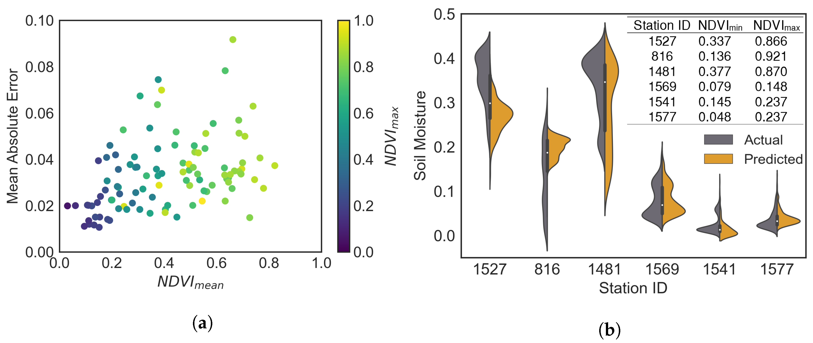
The presence of biomass over soil may affect the model’s prediction capability because the satellite data also carries information regarding the vegetation. To see the effect of the biomass, we calculated the NDVI from the S2 surface reflectance image during the testing periods and compared it with the MAE values of the model for the prediction dates.

Figure 7a visualizes the distribution of MAE values for all available stations together with the NDVI${}_{mean}$ and NDVI${}_{max}$ values. The figure shows the correlation between the mean NDVI${}_{mean}$ and MAE values. MAE values tend to increase with increasing NDVI${}_{mean}$ values.

The violin plot given in Figure 7b shows the distribution of the actual vs. predicted SM values at stations whose MAE values are lower (Station ID: 1569, 1541, 1577) with low soil moisture and higher (Station ID: 1527, 816, 1481) with high soil moisture. Here, we focused on finding out the origins of the variations in MAE values among these stations. For this purpose, the variation of the NDVI values were used. This analysis showed that the NDVI variation is one of the reasons for the deterioration of the SM prediction.

The backscattered signals obtained from SAR data were strongly affected by high biomass due to the interaction between electromagnetic radiation, plants, and soil. Therefore, these findings show that the model’s estimation performance is prone to uncertainties from the existing biomass. Similar findings also exist in previous studies [35,71,72,73]. These studies found that the SM content in bare or low-density vegetation areas is more predictable than in high-density vegetation areas.

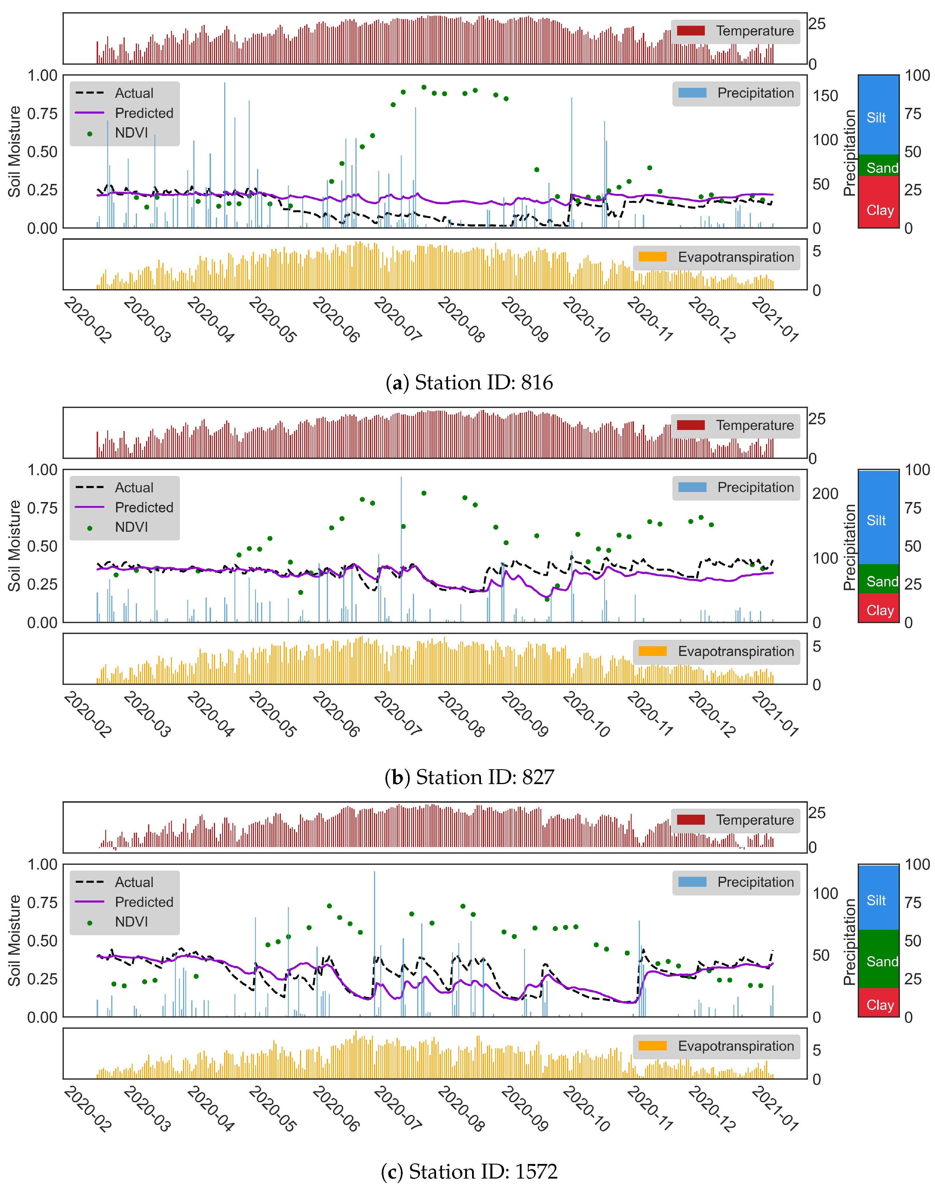
Another investigation that we conducted on the impact of NDVI variation was using station-based time series. For this purpose, we focused on some stations that show a variation in NDVI over the years. We see that the growth cycle of NDVI values before seeding and after harvest is lower than crops’ vegetative and reproductive phases. We believe that the prediction capability of the model thoughout the growth cycle is an important detail that needs to be investigated. Hence, we prepared the Figure 8a to show the model’s performance in time. According to Figure 8a, the model’s performance on the SM forecasting dropped approximately between May 2020 to October 2020 due to very low SM values. During this period, we can see an increase in the NDVI values from ∼0.2 to ∼0.9. We observed a similar situation in the other stations as well. In the time series of stations 827 and 1572, given in Figure 8b,c, the station has higher NDVI values from June to the end of December and from mid-April to the beginning of November, respectively. These three stations and the others with similar behavior have MAE values less than $0.075$.

5.3. Relationship between Model Performance and Soil Texture

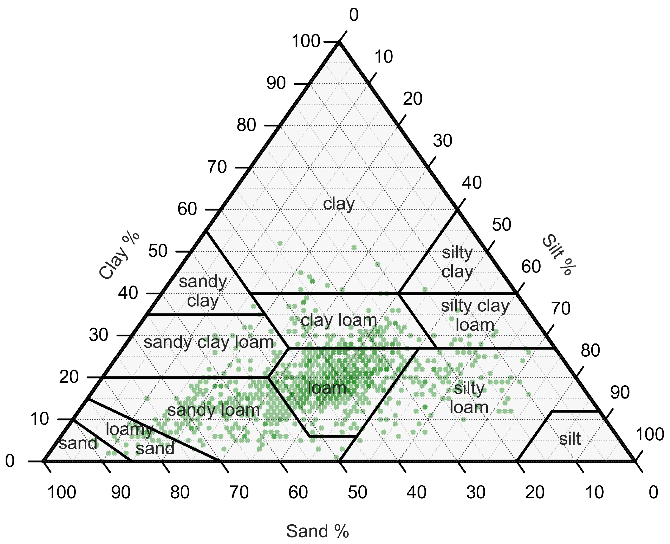
The variation in the soil texture is a driving factor for the spatial and temporal changes in the SM. Soils with high clay or silt fraction are associated with high water-holding capacity, resulting in a generally higher SM value. On the other hand, such soils lose their moisture slower than the others. From an agricultural point of view, clay soils have the highest soil moisture content in general; however, silty soils are more favorable for plants.

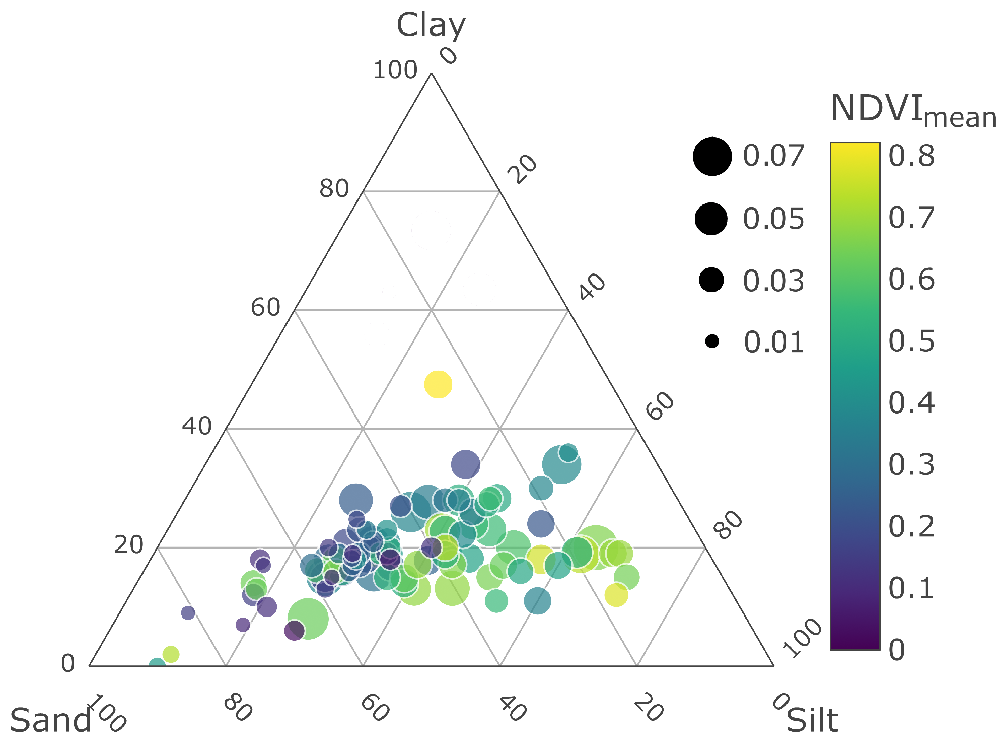
We provide a ternary plot in Figure 9 to show the MAE values of stations, which are scattered based on their soil texture contents. In the same figure, we also included each station’s NDVI${}_{mean}$ values in a color map. The combination of soil texture and NDVI${}_{mean}$ allows us to observe the relationship between the amount of silt and clay in the soil and vegetation activity.

The size of each circle, representing a station, is proportional to its MAE value. We observe that the smaller circles generally accumulate in areas where the sand fraction is high. Among all the stations, 61% have sandy soil with an average MAE of $0.03$, and 38% of them are silty soils with $0.04$ average MAE.

As we focus on particular stations for an in-depth investigation, it was observed that the silt content of the stations, having cropland cover, given in Figure 8 are 52%, 61%, and 42% for stations 816, 827, and 1572, respectively. In the corresponding stations, we have similar findings that justify the performance of the model w.r.t. the change in the NDVI values.

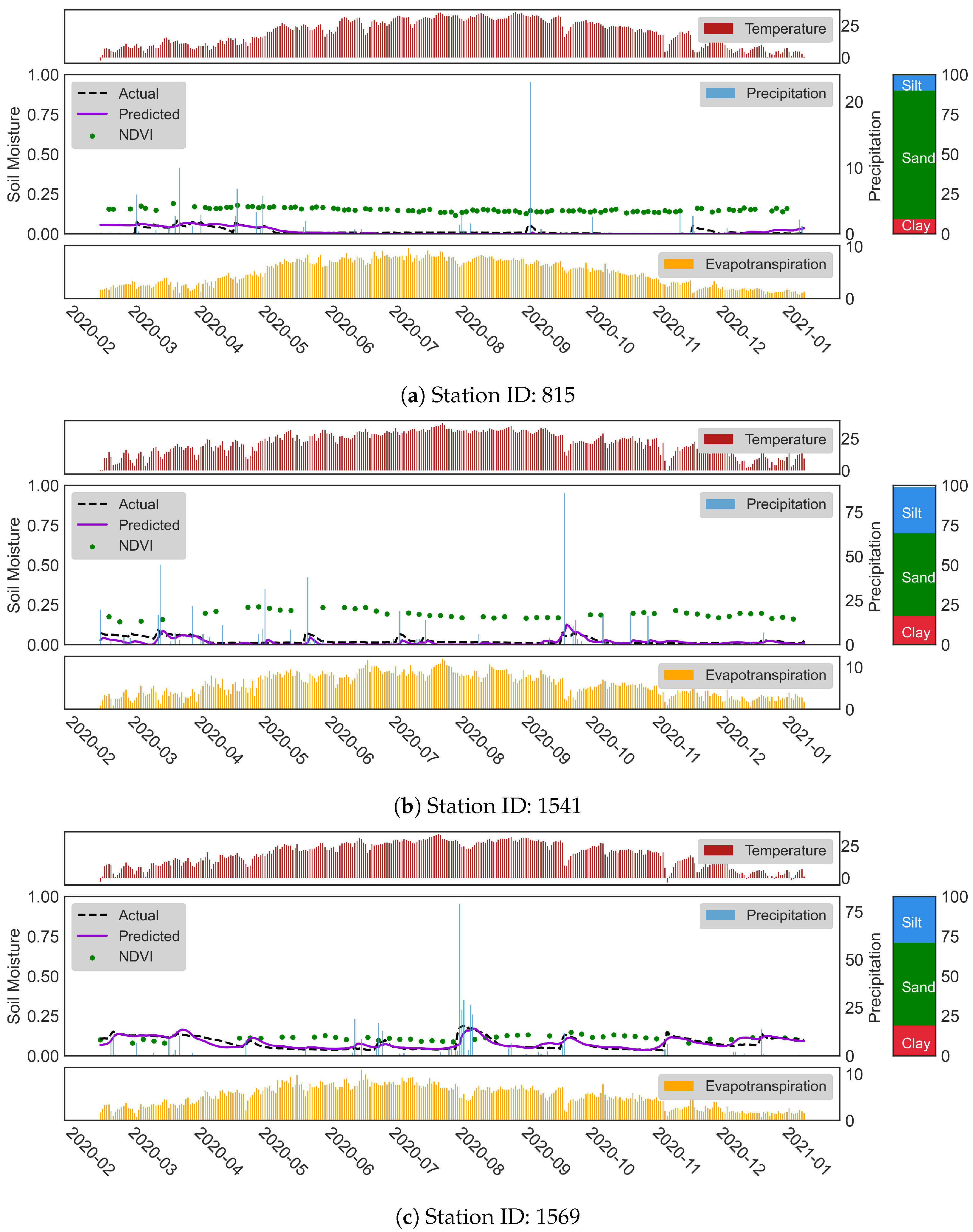
In addition to silt and clay-dominated soils, the soil types in which the sand proportion is higher generally have a lower trend in SM values because the sandy soil has low water-holding capacity. This property makes them less suitable for agricultural applications. In order to investigate the sand effect, we present the time series of SM predictions at stations 815, 1541, and 1569 in Figure 10. The typical features of these stations are the high percentage of sand fraction in soil content (81%, 52%, and 52% for stations 815, 1541, and 1569) and lower NDVI values along the time series. The mean NDVI value for these stations is 0.15, 0.19, and 0.11, respectively. Unlike the findings from Figure 8, we saw that in Figure 10a, the higher sand fraction leads to lower and less fluctuated SM values. Thus, the highest accuracy was obtained at stations with sandy soils having low NDVI values.

5.4. Relationship between Model Performance and Climate Classes

Lastly, we investigated the effect of climate classes. To this aim, we used [59], which defines four classes in total: tropical (A), dry (B), temperate (C), and continental (D). Our selected stations are distributed as $23\%$ in class B and $75\%$ in class C. The remaining $2\%$ belongs to classes A and D, with one station for each.

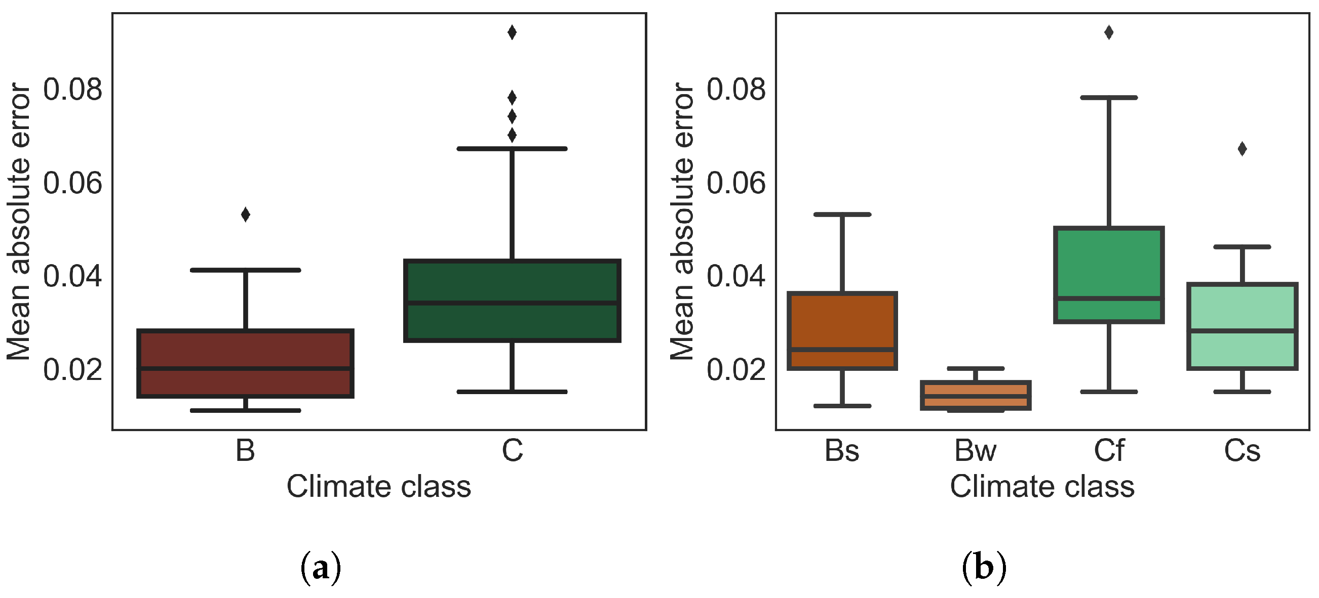
In Figure 11, we present the model’s prediction performance under different climate conditions as a boxplot. The stations in class B shows lower MAE values compared to those in class C (see Figure 11a). Considering the climate class properties, the rapid changes in the moisture affect the dielectric properties of the target [32,74]; at the same time, precipitation is a significant factor that negatively impacts the SM prediction due to the change in the interaction between SAR signals and land surface.

We obtained better soil moisture predictions in arid climates (Bw) than those in semi-arid climates (Bs) regions due to less precipitation and more evapotranspiration. We also observed a similar behavior between no-dry-season climate (Cf) and dry summer (Cs) temperate climate classes (see Figure 11b). The no-dry-season climate, as inferred by its name, has a high precipitation rate compared to a dry summer climate, which makes the stations located in this climate region challenging for SM prediction.

6. Conclusions

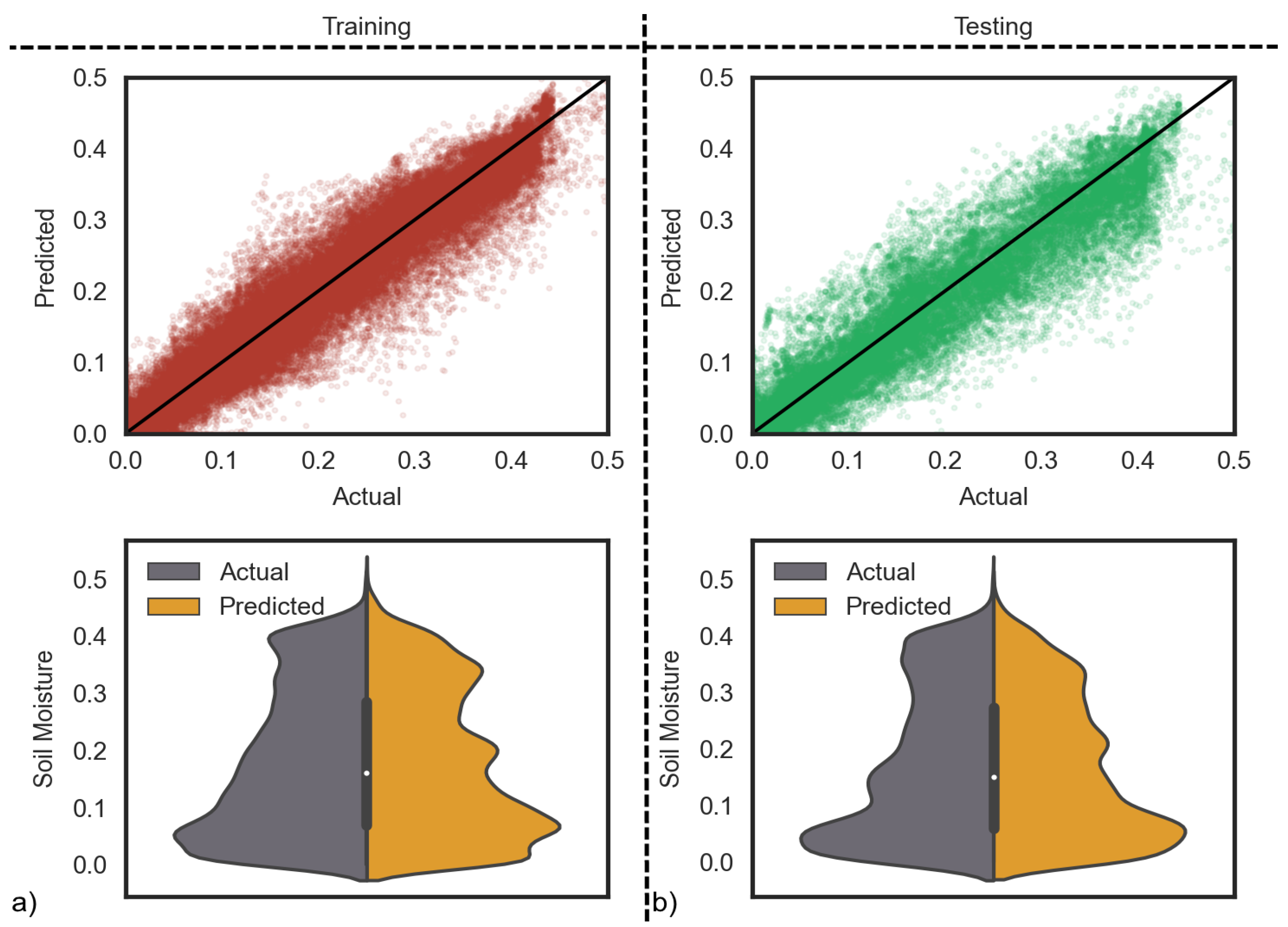
In this study, we investigated the short-term SM prediction based on satellite-derived data with LSTM. For this purpose, the static and dynamic features were combined to create sequential input data and used in situ SM measurements of 103 stations from ISMN as an output to train an LSTM model. Our approach uses soil texture and topographical data as static features and satellite (S1 and SMAP) and climate data as dynamic features. As SM monitoring is crucial for water resource management, we employed the SAR data due to its lower sensitivity to atmospheric conditions than optical data. To optimize the LSTM models’ hyperparameters, we used the gridSearchCV algorithm. After the optimization, the overall testing accuracy of the model was calculated as $R^2=0.87$, $RMSE=0.046$, and $MAE=0.033$. The values obtained from different stations are summarized in Appendix A, including the station ID, network and station name, soil texture, NDVI mean and max values, climate, land cover classes, and the corresponding MAE values.

During our investigations, it was observed that the model’s prediction performance is affected by the soil texture, vegetation status, and climate conditions. Variations in soil texture change the soil water-holding capacity. In the case in which the amount of sand was dominant, the SM values were easier to model than in the case of silt and clay dominance due to the low SM values and fewer fluctuations in sandy soils. We also observed that vegetation affects the interaction between the SAR signal and the soil. Thus, the model’s prediction ability was lowered in vegetated areas with high NDVI values. Moreover, the model can predict better under dry climate conditions, such as arid and semi-arid climates in relatively low precipitation.

This study used satellite-based products to create a model to forecast SM values. For operational purposes, we know that obtaining soil texture data on the pixel level is challenging. However, we can overcome this by conducting an intensive sampling campaign for soil texture, or existing models can be used [75], which employs S1 and S2 multi-temporal data.

In the future, we plan to combine the LSTM model with the attention mechanism to study the contribution of each variable to SM prediction. The LSTM model combined with the attention mechanism can determine the importance of each feature and its temporal relationship with SM phenomena. Thus, we can increase the accuracy of the model predictions and explain the physical behavior of the black-box model.

References

1. Jung, H.C.; Kang, D.H.; Kim, E.; Getirana, A.; Yoon, Y.; Kumar, S.; Peters-lidard, C.D.; Hwang, E. Towards a soil moisture drought monitoring system for South Korea. J. Hydrol. 2020, 589, 125176. [Google Scholar] [CrossRef]
2. Berg, A.; Sheffield, J. Climate change and drought: The soil moisture perspective. Curr. Clim. Chang. Rep. 2018, 4, 180–191. [Google Scholar] [CrossRef]
3. Norbiato, D.; Borga, M.; Degli Esposti, S.; Gaume, E.; Anquetin, S. Flash flood warning based on rainfall thresholds and soil moisture conditions: An assessment for gauged and ungauged basins. J. Hydrol. 2008, 362, 274–290. [Google Scholar] [CrossRef]
4. Martínez-Fernández, J.; González-Zamora, A.; Sánchez, N.; Gumuzzio, A.; Herrero-Jiménez, C. Satellite soil moisture for agricultural drought monitoring: Assessment of the SMOS derived Soil Water Deficit Index. Remote Sens. Environ. 2016, 177, 277–286. [Google Scholar] [CrossRef]
5. Efremova, N.; Seddik, M.E.A.; Erten, E. Soil Moisture Estimation using Sentinel-1/-2 Imagery Coupled with cycleGAN for Time-series Gap Filing. IEEE Trans. Geosci. Remote Sens. 2021, 60, 1–11. [Google Scholar] [CrossRef]
6. Lawless, C.; Semenov, M.A.; Jamieson, P.D. Quantifying the effect of uncertainty in soil moisture characteristics on plant growth using a crop simulation model. Field Crop. Res. 2008, 106, 138–147. [Google Scholar] [CrossRef]
7. Dai, X.; Huo, Z.; Wang, H. Simulation for response of crop yield to soil moisture and salinity with artificial neural network. Field Crop. Res. 2011, 121, 441–449. [Google Scholar] [CrossRef]
8. Famiglietti, J.; Rudnicki, J.; Rodell, M. Variability in surface moisture content along a hillslope transect: Rattlesnake Hill, Texas. J. Hydrol. 1998, 210, 259–281. [Google Scholar] [CrossRef] [Green Version]
9. Western, A.W.; Grayson, R.B.; Blöschl, G.; Willgoose, G.R.; McMahon, T.A. Observed spatial organization of soil moisture and its relation to terrain indices. Water Resour. Res. 1999, 35, 797–810. [Google Scholar] [CrossRef] [Green Version]
10. Moeslund, J.E.; Arge, L.; Bøcher, P.K.; Dalgaard, T.; Odgaard, M.V.; Nygaard, B.; Svenning, J.C. Topographically controlled soil moisture is the primary driver of local vegetation patterns across a lowland region. Ecosphere 2013, 4, art91. [Google Scholar] [CrossRef]
11. Gwak, Y.; Kim, S. Factors affecting soil moisture spatial variability for a humid forest hillslope. Hydrol. Process. 2017, 31, 431–445. [Google Scholar] [CrossRef]
12. Vereecken, H.; Kamai, T.; Harter, T.; Kasteel, R.; Hopmans, J.; Vanderborght, J. Explaining soil moisture variability as a function of mean soil moisture: A stochastic unsaturated flow perspective. Geophys. Res. Lett. 2007, 34, L22402. [Google Scholar] [CrossRef] [Green Version]
13. Rosenbaum, U.; Bogena, H.R.; Herbst, M.; Huisman, J.A.; Peterson, T.J.; Weuthen, A.; Western, A.W.; Vereecken, H. Seasonal and event dynamics of spatial soil moisture patterns at the small catchment scale. Water Resour. Res. 2012, 48, 2011WR011518. [Google Scholar] [CrossRef] [Green Version]
14. Wilson, D.J.; Western, A.W.; Grayson, R.B. Identifying and quantifying sources of variability in temporal and spatial soil moisture observations. Water Resour. Res. 2004, 40. [Google Scholar] [CrossRef]
15. Teuling, A.J.; Hupet, F.; Uijlenhoet, R.; Troch, P.A. Climate variability effects on spatial soil moisture dynamics. Geophys. Res. Lett. 2007, 34, L06406. [Google Scholar] [CrossRef]
16. Wang, T.; Franz, T.E.; Li, R.; You, J.; Shulski, M.D.; Ray, C. Evaluating climate and soil effects on regional soil moisture spatial variability using EOFs. Water Resour. Res. 2017, 53, 4022–4035. [Google Scholar] [CrossRef]
17. Liu, M.; Huang, C.; Wang, L.; Zhang, Y.; Luo, X. Short-term soil moisture forecasting via Gaussian process regression with sample selection. Water 2020, 12, 3085. [Google Scholar] [CrossRef]
18. Yu, J.; Zhang, X.; Xu, L.; Dong, J.; Zhangzhong, L. A hybrid CNN-GRU model for predicting soil moisture in maize root zone. Agric. Water Manag. 2021, 245, 106649. [Google Scholar] [CrossRef]
19. Li, Q.; Zhu, Y.; Shangguan, W.; Wang, X.; Li, L.; Yu, F. An attention-aware LSTM model for soil moisture and soil temperature prediction. Geoderma 2022, 409, 115651. [Google Scholar] [CrossRef]
20. O, S.; Orth, R. Global soil moisture data derived through machine learning trained with in-situ measurements. Sci. Data 2021, 8, 170. [Google Scholar] [CrossRef]
21. Souissi, R.; Zribi, M.; Corbari, C.; Mancini, M.; Muddu, S.; Tomer, S.K.; Upadhyaya, D.B.; Al Bitar, A. Integrating process-related information into an artificial neural network for root-zone soil moisture prediction. Hydrol. Earth Syst. Sci. 2022, 26, 3263–3297. [Google Scholar] [CrossRef]
22. Dobson, M.; Ulaby, F. Active Microwave Soil Moisture Research. IEEE Trans. Geosci. Remote Sens. 1986, GE-24, 23–36. [Google Scholar] [CrossRef]
23. Njoku, E.G.; Entekhabi, D. Passive microwave remote sensing of soil moisture. J. Hydrol. 1996, 184, 101–129. [Google Scholar] [CrossRef]
24. Entekhabi, D.; Njoku, E.G.; O’Neill, P.E.; Kellogg, K.H.; Crow, W.T.; Edelstein, W.N.; Entin, J.K.; Goodman, S.D.; Jackson, T.J.; Johnson, J.; et al. The Soil Moisture Active Passive (SMAP) Mission. Proc. IEEE 2010, 98, 704–716. [Google Scholar] [CrossRef]
25. Kerr, Y.H.; Waldteufel, P.; Richaume, P.; Wigneron, J.P.; Ferrazzoli, P.; Mahmoodi, A.; Bitar, A.A.; Cabot, F.; Gruhier, C.; Juglea, S.E.; et al. The SMOS Soil Moisture Retrieval Algorithm. IEEE Trans. Geosci. Remote Sens. 2012, 50, 1384–1403. [Google Scholar] [CrossRef]
26. Sadri, S.; Pan, M.; Wada, Y.; Vergopolan, N.; Sheffield, J.; Famiglietti, J.S.; Kerr, Y.; Wood, E. A global near-real-time soil moisture index monitor for food security using integrated SMOS and SMAP. Remote Sens. Environ. 2020, 246, 111864. [Google Scholar] [CrossRef]
27. Peng, J.; Niesel, J.; Loew, A. Evaluation of soil moisture downscaling using a simple thermal-based proxy—The REMEDHUS network (Spain) example. Hydrol. Earth Syst. Sci. 2015, 19, 4765–4782. [Google Scholar] [CrossRef] [Green Version]
28. Peng, J.; Loew, A.; Zhang, S.; Wang, J.; Niesel, J. Spatial Downscaling of Satellite Soil Moisture Data Using a Vegetation Temperature Condition Index. IEEE Trans. Geosci. Remote Sens. 2016, 54, 558–566. [Google Scholar] [CrossRef]
29. Hornacek, M.; Wagner, W.; Sabel, D.; Truong, H.L.; Snoeij, P.; Hahmann, T.; Diedrich, E.; Doubkova, M. Potential for High Resolution Systematic Global Surface Soil Moisture Retrieval via Change Detection Using Sentinel-1. IEEE J. Sel. Top. Appl. Earth Obs. Remote Sens. 2012, 5, 1303–1311. [Google Scholar] [CrossRef]
30. Gao, Q.; Zribi, M.; Escorihuela, M.J.; Baghdadi, N. Synergetic use of Sentinel-1 and Sentinel-2 data for soil moisture mapping at 100 m resolution. Sensors 2017, 17, 1966. [Google Scholar] [CrossRef]
31. Liu, Z.; Li, P.; Yang, J. Soil Moisture Retrieval and Spatiotemporal Pattern Analysis Using Sentinel-1 Data of Dahra, Senegal. Remote Sens. 2017, 9, 1197. [Google Scholar] [CrossRef] [Green Version]
32. Fan, D.; Zhao, T.; Jiang, X.; Xue, H.; Moukomla, S.; Kuntiyawichai, K.; Shi, J. Soil Moisture Retrieval From Sentinel-1 Time-Series Data Over Croplands of Northeastern Thailand. IEEE Geosci. Remote Sens. Lett. 2022, 19, 1–5. [Google Scholar] [CrossRef]
33. Nguyen, H.H.; Cho, S.; Jeong, J.; Choi, M. A D-vine copula quantile regression approach for soil moisture retrieval from dual polarimetric SAR Sentinel-1 over vegetated terrains. Remote Sens. Environ. 2021, 255, 112283. [Google Scholar] [CrossRef]
34. Attarzadeh, R.; Amini, J.; Notarnicola, C.; Greifeneder, F. Synergetic Use of Sentinel-1 and Sentinel-2 Data for Soil Moisture Mapping at Plot Scale. Remote Sens. 2018, 10, 1285. [Google Scholar] [CrossRef] [Green Version]
35. Greifeneder, F.; Notarnicola, C.; Wagner, W. A machine learning-based approach for surface soil moisture estimations with google earth engine. Remote Sens. 2021, 13, 2099. [Google Scholar] [CrossRef]
36. Xue, Z.; Zhang, Y.; Zhang, L.; Li, H. Ensemble Learning Embedded with Gaussian Process Regression for Soil Moisture Estimation: A Case Study of the Continental U.S. IEEE Trans. Geosci. Remote Sens. 2022, 60, 4508817. [Google Scholar] [CrossRef]
37. Lei, F.; Senyurek, V.; Kurum, M.; Gurbuz, A.C.; Boyd, D.; Moorhead, R.; Crow, W.T.; Eroglu, O. Quasi-global machine learning-based soil moisture estimates at high spatio-temporal scales using CYGNSS and SMAP observations. Remote Sens. Environ. 2022, 276, 113041. [Google Scholar] [CrossRef]
38. Ali, I.; Greifeneder, F.; Stamenkovic, J.; Neumann, M.; Notarnicola, C. Review of Machine Learning Approaches for Biomass and Soil Moisture Retrievals from Remote Sensing Data. Remote Sens. 2015, 7, 16398–16421. [Google Scholar] [CrossRef] [Green Version]
39. Yuan, Q.; Shen, H.; Li, T.; Li, Z.; Li, S.; Jiang, Y.; Xu, H.; Tan, W.; Yang, Q.; Wang, J.; et al. Deep learning in environmental remote sensing: Achievements and challenges. Remote Sens. Environ. 2020, 241, 111716. [Google Scholar] [CrossRef]
40. El Hajj, M.; Baghdadi, N.; Zribi, M.; Bazzi, H. Synergic use of Sentinel-1 and Sentinel-2 images for operational soil moisture mapping at high spatial resolution over agricultural areas. Remote Sens. 2017, 9, 1292. [Google Scholar] [CrossRef]
41. Hegazi, E.H.; Yang, L.; Huang, J. A Convolutional Neural Network Algorithm for Soil Moisture Prediction from Sentinel-1 SAR Images. Remote Sens. 2021, 13, 4964. [Google Scholar] [CrossRef]
42. Chung, J.; Lee, Y.; Kim, J.; Jung, C.; Kim, S. Soil Moisture Content Estimation Based on Sentinel-1 SAR Imagery Using an Artificial Neural Network and Hydrological Components. Remote Sens. 2022, 14, 465. [Google Scholar] [CrossRef]
43. Chaudhary, S.K.; Srivastava, P.K.; Gupta, D.K.; Kumar, P.; Prasad, R.; Pandey, D.K.; Das, A.K.; Gupta, M. Machine learning algorithms for soil moisture estimation using Sentinel-1: Model development and implementation. Adv. Space Res. 2022, 69, 1799–1812. [Google Scholar] [CrossRef]
44. Cui, H.; Jiang, L.; Paloscia, S.; Santi, E.; Pettinato, S.; Wang, J.; Fang, X.; Liao, W. The Potential of ALOS-2 and Sentinel-1 Radar Data for Soil Moisture Retrieval With High Spatial Resolution Over Agroforestry Areas, China. IEEE Trans. Geosci. Remote Sens. 2022, 60, 4402617. [Google Scholar] [CrossRef]
45. Nativel, S.; Ayari, E.; Rodriguez-Fernandez, N.; Baghdadi, N.; Madelon, R.; Albergel, C.; Zribi, M. Hybrid Methodology Using Sentinel-1/Sentinel-2 for Soil Moisture Estimation. Remote Sens. 2022, 14, 2434. [Google Scholar] [CrossRef]
46. Eroglu, O.; Kurum, M.; Boyd, D.; Gurbuz, A.C. High Spatio-Temporal Resolution CYGNSS Soil Moisture Estimates Using Artificial Neural Networks. Remote Sens. 2019, 11, 2272. [Google Scholar] [CrossRef] [Green Version]
47. Hachani, A.; Ouessar, M.; Paloscia, S.; Santi, E.; Pettinato, S. Soil moisture retrieval from Sentinel-1 acquisitions in an arid environment in Tunisia: Application of Artificial Neural Networks techniques. Int. J. Remote Sens. 2019, 40, 9159–9180. [Google Scholar] [CrossRef]
48. suk Lee, C.; Sohn, E.; Park, J.D.; Jang, J.D. Estimation of soil moisture using deep learning based on satellite data: A case study of South Korea. Gisci. Remote Sens. 2019, 56, 43–67. [Google Scholar] [CrossRef]
49. Pascanu, R.; Mikolov, T.; Bengio, Y. On the difficulty of training recurrent neural networks. In Proceedings of the International Conference on Machine Learning, Atlanta, GA, USA, 16–21 June 2013; pp. 1310–1318. [Google Scholar]
50. Hochreiter, S.; Schmidhuber, J. Long short-term memory. Neural Comput. 1997, 9, 1735–1780. [Google Scholar] [CrossRef]
51. Fang, K.; Shen, C.; Kifer, D.; Yang, X. Prolongation of SMAP to spatiotemporally seamless coverage of continental US using a deep learning neural network. Geophys. Res. Lett. 2017, 44, 11–030. [Google Scholar] [CrossRef]
52. Fang, K.; Pan, M.; Shen, C. The value of SMAP for long-term soil moisture estimation with the help of deep learning. IEEE Trans. Geosci. Remote Sens. 2018, 57, 2221–2233. [Google Scholar] [CrossRef]
53. Fang, K.; Shen, C. Near-Real-Time Forecast of Satellite-Based Soil Moisture Using Long Short-Term Memory with an Adaptive Data Integration Kernel. J. Hydrometeorol. 2020, 21, 399–413. [Google Scholar] [CrossRef]
54. Ming, W.; Ji, X.; Zhang, M.; Li, Y.; Liu, C.; Wang, Y.; Li, J. A Hybrid Triple Collocation-Deep Learning Approach for Improving Soil Moisture Estimation from Satellite and Model-Based Data. Remote Sens. 2022, 14, 1744. [Google Scholar] [CrossRef]
55. Dorigo, W.; Wagner, W.; Hohensinn, R.; Hahn, S.; Paulik, C.; Xaver, A.; Gruber, A.; Drusch, M.; Mecklenburg, S.; van Oevelen, P.; et al. The International Soil Moisture Network: A data hosting facility for global in situ soil moisture measurements. Hydrol. Earth Syst. Sci. 2011, 15, 1675–1698. [Google Scholar] [CrossRef] [Green Version]
56. Dorigo, W.; Himmelbauer, I.; Aberer, D.; Schremmer, L.; Petrakovic, I.; Zappa, L.; Preimesberger, W.; Xaver, A.; Annor, F.; Ardö, J.; et al. The International Soil Moisture Network: Serving Earth system science for over a decade. Hydrol. Earth Syst. Sci. 2021, 25, 5749–5804. [Google Scholar] [CrossRef]
57. Montzka, C.; Bogena, H.R.; Herbst, M.; Cosh, M.H.; Jagdhuber, T.; Vereecken, H. Estimating the Number of Reference Sites Necessary for the Validation of Global Soil Moisture Products. IEEE Geosci. Remote Sens. Lett. 2021, 18, 1530–1534. [Google Scholar] [CrossRef]
58. European Space Agency. Land Cover CCI Product User Guide Version 2 Tech. Rep. 2017. Available online: http://maps.elie.ucl.ac.be/CCI/viewer/download/ESACCI-LC-Ph2-PUGv2_2.0.pdf (accessed on 18 July 2022).
59. Rubel, F.; Brugger, K.; Haslinger, K.; Auer, I. The climate of the European Alps: Shift of very high resolution Köppen-Geiger climate zones 1800–2100. Meteorologische Zeitschrift 2017, 26, 115–125. [Google Scholar] [CrossRef]
60. Gorelick, N.; Hancher, M.; Dixon, M.; Ilyushchenko, S.; Thau, D.; Moore, R. Google Earth Engine: Planetary-scale geospatial analysis for everyone. Remote Sens. Environ. 2017, 202, 18–27. [Google Scholar] [CrossRef]
61. Liu, Y.; Qian, J.; Yue, H. Combined Sentinel-1A with Sentinel-2A to Estimate Soil Moisture in Farmland. IEEE J. Sel. Top. Appl. Earth Obs. Remote Sens. 2021, 14, 1292–1310. [Google Scholar] [CrossRef]
62. Baghdadi, N.N.; El Hajj, M.; Zribi, M.; Fayad, I. Coupling SAR C-Band and Optical Data for Soil Moisture and Leaf Area Index Retrieval Over Irrigated Grasslands. IEEE J. Sel. Top. Appl. Earth Obs. Remote Sens. 2016, 9, 1229–1243. [Google Scholar] [CrossRef]
63. Bazzi, H.; Baghdadi, N.; El Hajj, M.; Zribi, M.; Belhouchette, H. A Comparison of Two Soil Moisture Products S2MP and Copernicus-SSM Over Southern France. IEEE J. Sel. Top. Appl. Earth Obs. Remote Sens. 2019, 12, 3366–3375. [Google Scholar] [CrossRef]
64. Liang, J.; Liang, G.; Zhao, Y.; Zhang, Y. A synergic method of Sentinel-1 and Sentinel-2 images for retrieving soil moisture content in agricultural regions. Comput. Electron. Agric. 2021, 190, 106485. [Google Scholar] [CrossRef]
65. Palmisano, D.; Satalino, G.; Balenzano, A.; Mattia, F. Coherent and Incoherent Change Detection for Soil moisture retrieval from Sentinel-1 data. IEEE Geosci. Remote Sens. Lett. 2022, 19, 2503805. [Google Scholar] [CrossRef]
66. Entekhabi, D.; Yueh, S.; O’Neill, P.; Kellogg, K.; Allen, A.; Bindlish, R.; Brown, M.; Chan, S.; Colliander, A.; Crow, W.; et al. SMAP Handbook Soil Moisture Active Passive: Mapping Soil Moisture Freeze/Thaw from Space; JPL Publication: Pasadena, CA, USA, 2014. [Google Scholar]
67. Takaku, J.; Tadono, T.; Tsutsui, K. Generation of high-resolution global DSM from ALOS Prism. In Proceedings of the International Archives of the Photogrammetry, Remote Sensing and Spatial Information Sciences, Suzhou, China, 14–16 May 2014. [Google Scholar]
68. Longden, A.J. Meteomatics. In Proceedings of the 102nd American Meteorological Society Annual Meeting, Houston, TX, USA, 23–27 January 2022. [Google Scholar]
69. Goodfellow, I.; Bengio, Y.; Courville, A. Deep Learning; MIT Press: Cambridge, MA, USA, 2016. [Google Scholar]
70. Sun, R.Y. Optimization for Deep Learning: An Overview. J. Oper. Res. Soc. China 2020, 8, 249–294. [Google Scholar] [CrossRef]
71. Bai, J.; Cui, Q.; Zhang, W.; Meng, L. An approach for downscaling SMAP soil moisture by combining Sentinel-1 SAR and MODIS data. Remote Sens. 2019, 11, 2736. [Google Scholar] [CrossRef] [Green Version]
72. Millard, K.; Richardson, M. Quantifying the relative contributions of vegetation and soil moisture conditions to polarimetric C-Band SAR response in a temperate peatland. Remote Sens. Environ. 2018, 206, 123–138. [Google Scholar] [CrossRef]
73. Çelik, M.F.; Erten, E. Biophysical parameter estimation of crops from polarimetric synthetic aperture radar imagery with data-driven polynomial chaos expansion and global sensitivity analysis. Comput. Electron. Agric. 2022, 194, 106781. [Google Scholar] [CrossRef]
74. Benninga, H.J.F.; van der Velde, R.; Su, Z. Impacts of radiometric uncertainty and weather-related surface conditions on soil moisture retrievals with Sentinel-1. Remote Sens. 2019, 11, 2025. [Google Scholar] [CrossRef] [Green Version]
75. Yuzugullu, O.; Lorenz, F.; Fröhlich, P.; Liebisch, F. Understanding Fields by Remote Sensing: Soil Zoning and Property Mapping. Remote Sens. 2020, 12, 1116. [Google Scholar] [CrossRef]
Figure 1. The spatial distribution of ISMN sites. Red dots display the distribution of 103 stations with reliable data.
Remotesensing 14 05584 g001
Figure 2. Ternary plot of the soil class distribution of ISMN sites.
Remotesensing 14 05584 g002
Figure 3. The overall process chart of the study, starting from data sources and ending with the final-user output.
Remotesensing 14 05584 g003
Figure 4. Accuracy of the best-performing LSTM model according to epoch. The upper figure shows the training progress of the model w.r.t. loss value per epoch, and the lower figure shows the change in accuracy w.r.t. R 2 and RMSE.
Remotesensing 14 05584 g004
Figure 5. The scatter plot (top left and right) and distribution graph (bottom left and right) of (a) training and (b) testing data of windows size 5.
Remotesensing 14 05584 g005
Figure 6. Overall MAE for land cover classes.
Remotesensing 14 05584 g006
Figure 7. Model performance w.r.t. NDVI variation. (a) Scatter plot shows the distribution of MAE vs. NDVI relationship for each station. (b) Violin plots representing the statistical distribution of actual and predicted temporal SM data at the ISMN stations with their minimum and maximum NDVI values.
Remotesensing 14 05584 g007
Figure 8. Time series of SM predictions during the testing period for stations 816, 827, and 1572.
Remotesensing 14 05584 g008
Figure 9. Soil texture ternary plot w.r.t. MAE of each station. The circles are scaled based on their MAE value and are colored based on NDVI m e a n .
Remotesensing 14 05584 g009
Figure 10. Time series of SM predictions during the testing period for stations 815, 1541, and 1569.
Remotesensing 14 05584 g010
Figure 11. Overall mean absolute error for first-order (a) and second-order (b) Köppen–Geiger climate classes [59].
Remotesensing 14 05584 g011