Abstract
Remote sensing image scene classification has drawn extensive attention for its wide application in various scenarios. Scene classification in many practical cases faces the challenge of few-shot conditions. The major difficulty of few-shot remote sensing image scene classification is how to extract effective features from insufficient labeled data. To solve these issues, a multi-scale graph-based feature fusion (MGFF) model is proposed for few-shot remote sensing image scene classification. In the MGFF model, a graph-based feature construction model is developed to transform traditional image features into graph-based features, which aims to effectively represent the spatial relations among images. Then, a graph-based feature fusion model is proposed to integrate graph-based features of multiple scales, which aims to enhance sample discrimination based on different scale information. Experimental results on two public remote sensing datasets prove that the MGFF model can achieve superior accuracy than other few-shot scene classification approaches.
1. Introduction
Scene classification of a remote sensing image is a significant assignment, which has attracted significant attention in various applications. Recent years have witnessed the continuous improvement of imaging technology, then the resolution of remote sensing images has gradually increased, and more useful information can be captured from remote sensing images, including extensive land cover information, such as terrain, mountain, as well as water. For different scenes, remote sensing images are processed differently. It is of great significance to assign semantic labels to remote sensing images [1,2], which is helpful for the management and analysis the remote sensing data in a unified manner. Therefore, scene classification aims at classifying remote sensing images based on similar scene characteristics by extracted features [3]. Currently, scene classification technology has been broadly applied in geological exploration, planning management, environmental monitoring, object detection, and other fields [4,5]. The methods for remote sensing image scene classification consist of three types according to visual features, which are methods derived from low-level visual features, middle-level visual representations, and high-level visual information [6].
The classification methods based on low-level visual features obtain the structure, edge, and other basic information from images, where these features are extracted based on traditional hand-crafted methods. For example, scale-invariant feature transform (SIFT) [7] is used to obtain low-level visual features, which has been frequently adopted for the scene classification of remote sensing images. The spatial envelope feature algorithm [8] adopts global feature information to classify remote sensing images, which can represent the overall information of images macroscopically. Nevertheless, scene classification derived from the global feature information is difficult to handle complex scenarios of remote sensing images. Furthermore, low-level visual features contain less semantic information, which is challenging to obtain satisfactory results for scene classification with high complexity and non-uniform spaces.
The classification approaches derived from middle-level visual information encode the local features extracted by traditional manual approaches, and further optimize the feature representation with more recognition ability. Among middle-level feature based methods, bag-of-words model (BoVW) [9] is one of the most classic methods. BoVW model uses SIFT to extract local features from images, and then encodes local features into global features using visual word bags. Thus, BoVW combines various underlying visual features to enhance the performance of recognition ability of the model itself [10]. Many subsequent methods [11,12] that use multiple features to deal with the scene classification are developed based on BoVW. Although mid-level feature based methods achieve superior results than low-level feature based methods, they also face many shortcomings. In particular, the methods of re-representing local features will ignore the relationship among each local feature, which weaken the classification effect.
As for classification approaches derived from high-level visual information, they are mainly employing deep neural networks, which can learn more abstract semantic information from remote sensing images. Recent years have witnessed that the deep learning technology has greatly improve the performances in numerous visual assignments, and various convolutional neural networks, such as AlexNet [13], VGG-VD-16 [14], and GoogLeNet [15] have been proposed for image classification task. Penatti et al. [16] first adopted convolutional neural network to deal with scene classification of remote sensing image, which is proved to achieve superb results. Polarimetric-feature-driven deep CNN [17] is proposed to solve PolSAR classification with limited training samples. A convolutional neural network is used in the task of image scene classification, which is usually divided into three training methods. The first is complete training, which is conducted under the condition that all weight parameters of the network are initialized randomly, and good performance is obtained [18,19]. The second is to directly use the trained model as a feature extractor, and then use the extracted features in the scene classification task through algorithm processing [20]. The third is to transfer the trained parameters to the model to achieve better results [21]. Compared with approaches derived from low-level information, as well as middle-level information, classification derived from high-level visual features can completely express the deeper abstract semantic information of images, which is capable for enhancing the performance of scene classification.
Generally, classification methods based on deep learning technology require extensive labeled samples for network training. If the training samples are insufficient, deep model will face the problem of overfitting, which may result in a sharp decrease in the performance on the test set. As for most practical applications, it is quite challenging to collect extensive labeled samples, and collection of annotated samples often consumes a lot of time. Therefore, scene classification of remote sensing images in a few-shot case is of great significance. Inspired by human cognition of novel objects based on prior knowledge, few-shot learning has been developed to learn policies for recognition and classification with quite limited labeled samples [22,23]. At present, few-shot learning methods are mainly derived from meta learning, as well as transfer learning.
In contrast with optical images, remote sensing images possess the distinctions of large size, abundant data, and rich land cover information [24]. Since remote sensing images capture complex ground scenes, performance of scene classification will be affected by environmental factors and other factors [25]. Specifically, if there exist distinguished intra-class differences, remote sensing images of the same category may be classified into different categories, where intra-class variability arises because similar scenes contain large differences in underlying feature space. Furthermore, remote sensing images of different types may be classified into the same scene because they contain similar backgrounds or spatial structures, where this phenomenon is called as inter-class similarity. These issues, mentioned above, will reduce the efficacy for scene classification. In addition, traditional scene classification methods generally utilize deep features of the top layer for classification, but the front layer features still contain useful information. Such information may be lost during convolution or other operations. Therefore, the extraction of multi-scale feature is beneficial to expand the information from remote sensing images. How to utilize multi-scale features in a few-shot case is also an issue that needs to be resolved.
For few-shot scene classification of remote sensing images, a multi-scale graph-based feature fusion (MGFF) model is proposed, which aims at excavating effective features in few-shot cases. In our approach, we firstly pre-train a feature extractor to learn multi-scale features of remote sensing images, and then a transposed convolution is applied to correct the extracted multi-scale features. After that, image features are transformed into graph-based features based on the construction module. Finally, a graph-based feature fusion model is proposed to enhance sample discrimination based on different scale features. The major contributions of this paper are summarized as follows:
- A graph-based feature learning model is developed to learn features from remote sensing images firstly, which enables to effectively express the spatial relations among remote sensing images. It is able to take advantage of relation information for scene classification, which is beneficial to few-shot scene classification.
- A graph-based feature fusion model is proposed, which can integrate graph-based features of multiple scales. It is able to enhance sample discrimination based on different scale features, which integrates more abundant and effective semantic information. The proposed model can take full advantage of image features to improve few-shot classification accuracies, which reduces the influence of inconsistent semantic information.
- Experimental results on two public remote sensing data illustrate that the proposed MGFF yield an improvement of classification accuracy about 2–10% contrast to other advanced methods, which proves the efficacy of our MGFF model.
2. Related Works
In this section, related work related to remote sensing image scene classification, few-shot learning, and graph learning will be introduced in detail.
2.1. Remote Sensing Image Scene Classification
Although remote sensing image scene classification consists of three categories according to different visual features, classification derived from high-level information utilizes the powerful learning ability of deep neural network [26,27], which can excavate discriminative information from remote sensing images. Deeper abstract semantic information enables to boost the classification performance. Therefore, methods derived from deep learning are widely adopted to deal with the scene classification of remote sensing image [28,29,30].
In deep learning based methods, a convolutional neural network (CNN) has been broadly adopted for scene classification [31,32]. Nogueira et al. [33] applied a CNN to extract features and used linear SVM for scene classification. Cheng et al. [34] proposed a discriminative CNN to deal with the problem of misclassification due to factors of intra-class dissimilarity and inter-class similarity. Wang et al. [35] proposed an attention loop CNN model for scene classification, which can extract high-level feature information and guarantee effective discarding of non-critical information. Tang et al. [36] proposed class-level prototype guided multi-scale feature learning method, which enables to make a distinction from different semantics with limited labeled samples. Rafael Pires et al. [37] developed a transfer learning method to learn the effect of a CNN in dealing with the scene classification task, which demonstrates the feasibility of transfer learning from natural images to remote sensing images. Zeng et al. [38] proposed specific contrastive learning model, which enables to boost the scene classification accuracy with limited supervised samples. Although the above works make an effect on boosting the performance of remote sensing image scene classification, they all focus on extracting high-level visual features from remote sensing images, but low-level features and middle-level features also contain useful information. Therefore, multi-scale feature fusion should be considered to learn abundant information from different scale features.
2.2. Few-Shot Learning
In recent years, few-shot learning has drawn great attention, which aims to enhance the learning capacity on the novel categories with fewer labeled samples [39,40]. Few-shot learning has also been developed for remote sensing image scene classification, where various few-shot learning approaches have been widely applied [41,42]. The follow-up work is to design a more suitable few-shot learning method for remote sensing image scene classification. Alajaji et al. [43] proposed a prototype network, which combines with a pre-trained SqueezeNet to obtain better prototype features of each category. Jiang et al. [44] proposed a multi-scale metric learning (MSML) method, which extracts multi-scale features and learns the relations among samples for few-shot classification. Due to the issues of intra-class difference, as well as inter-class similarity in remote sensing images, prototype-based few-shot learning models ignore the verification of prototype features, which reduce the scene classification performance. To overcome these issues, Cheng et al. [45] proposed a Siamese prototype network (SPNet), which develops prototype self calibration and mutual calibration to optimize sample features. Zeng et al. [46] proposed an iterative distribution learning network, where three sub-modules are developed to improve the discrimination of features. In the network, the similarity distribution learning model is adopted to calculate the relationship of different instances, the label matching model is utilized as few-shot classifier derived from prior knowledge, and the attention-based feature calibration model is developed to optimize the sample features and yield the final features for the next iteration.
Meta learning is also adopted to few-shot scene classification. In [47], a meta learning based method named RS-MetaNet is proposed to learn a metric space through a series of assignments, which is suitable for scene classification with limited label data. Li et al. [48] proposed a discriminative learning based adaptive matching network (DLA-MatchNet), which is a few-shot learning method that adds a matcher into the feature extractor. In [49], a life-long few-shot learning model is proposed for few-shot classification, which realizes knowledge transferring from one dataset to a novel dataset.
2.3. Graph Learning
Graph learning aims to study how to apply deep neural networks on graph-based data, and has accomplished various classification tasks. In recent years, graph learning [50] has been adopted to few-shot learning tasks and realized effective results, where a series of graph neural networks (GNNs) have been proposed [51,52]. GNNs can utilize the available information of similar samples for classification.
Several recent studies have been proposed to enable the neural network to handle the graph structures [53]. In a graph convolutional network (GCN) [54], a graph convolution operator is introduced, which can be cascaded to obtain a deep learning architecture. A graph attention network (GAT) [55] extends the GCN model by adding a learnable attention kernel, which allows to assign different weights to the set of adjacent nodes. A simplified graph convolutional network (SGC) [56] optimizes the network structure by simplifying the non-linear transformation function to the single linear transformation function, which achieves superior results with fewer parameters. A graph-based embedding smoothing network (GES-Net) [57] adopts an unsupervised non-parametric regularizer, severed as embedding smoothing, which can obtain superb results for few-shot remote sensing image scene classification. Although the above works all use graph learning to solve classification tasks, the fusion of graph features may result in missing of useful information and reducing the stability of deep network. Therefore, effective utilization of a graph-based neural network needs to be studied to fully excavate the image features for enhancing few-shot scene classification performance.
3. Methodology
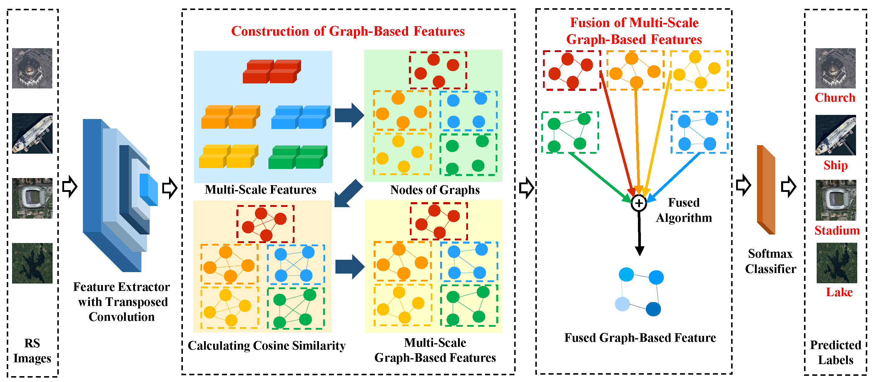
The proposed multi-scale graph-based feature fusion model is shown in Figure 1. In our framework, a pre-trained feature extractor is firstly adopted to extract multi-scale image features. Furthermore, a transposed convolution operation is applied to correct the extracted multi-scale features. After that, image features are transformed into graph-based features based on the construction module. Finally, a graph-based feature fusion model is proposed to enhance sample discrimination based on different scale features, which is utilized for scene classification.
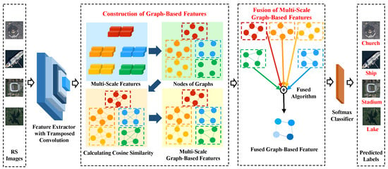
Figure 1.
The framework of proposed multi-scale graph-based feature fusion model.
3.1. Problem Formulation
The problem with few-shot remote sensing image scene classification is in utilizing an extremely limited number of labeled data for training a classifier. As for few-shot learning tasks, all the samples can be divided into two distinct datasets, named and , where there is no overlap in categories. In , each category includes abundant labeled data, which can be adopted for training and validation. However, in , there are only extremely limited number of labeled data of each class, which is applied for testing.
During the training and validation process, we split into four different parts without overlap in categories, namely, , , , , in which denotes the ith sample, and denotes corresponding label. and are applied during the training process. and are adopted during the validation process.
In the training process, the parameters of pre-trained feature extractor are updated on , and the evaluation of the classification module is conducted on . When the evaluation results tend to be stable, it can be considered that the feature extractor has been well trained. In the testing process, we can regard the classification as a M-way Z-shot K-query task, where Z labeled samples of each class (Z samples in total) are applied as the prior knowledge, and unlabeled samples are utilized for prediction. We split into two parts, which are (Z), and . The number of labeled samples is extremely small, where the shot number Z is set to 1 or 5 in the experiments.
3.2. Extraction of Multi-Scale Features
To extract multi-scale features from images, ResNet-12 is adopted as the backbone in our framework. ResNet-12 contains four residual convolution blocks and one average pooling layer. The structure of the backbone is shown in Figure 2. Each residual convolution block is composed of three convolution layers, batch normalization layers and ReLU layers, alternately.

Figure 2.
The structure of the backbone.
Considering the sample number of the training set is insufficient, data augmentation is utilized to extend pseudo training samples, where random rotation is applied to generate pseudo images. Thus, original images and generated images are used for deep network training. The loss function of backbone optimization is defined as follows:
where stands for the total loss, denotes cross-entropy loss function, represents the loss of original images, stands for the loss of the generated images, and is a hyperparameter in order to balance the two types of loss.
Considering the scarcity of samples, we prefer to improve our deep network from the perspective of sample feature enhancement. As for traditional classification methods, only the top layer features are utilized for final classification. However, the low-level features as well as mid-level features from deep neural network also contain useful information, which may be weakened or even disappeared during the convolution and pooling operations. Therefore, multi-scale feature fusion is beneficial to expand the information of image features.
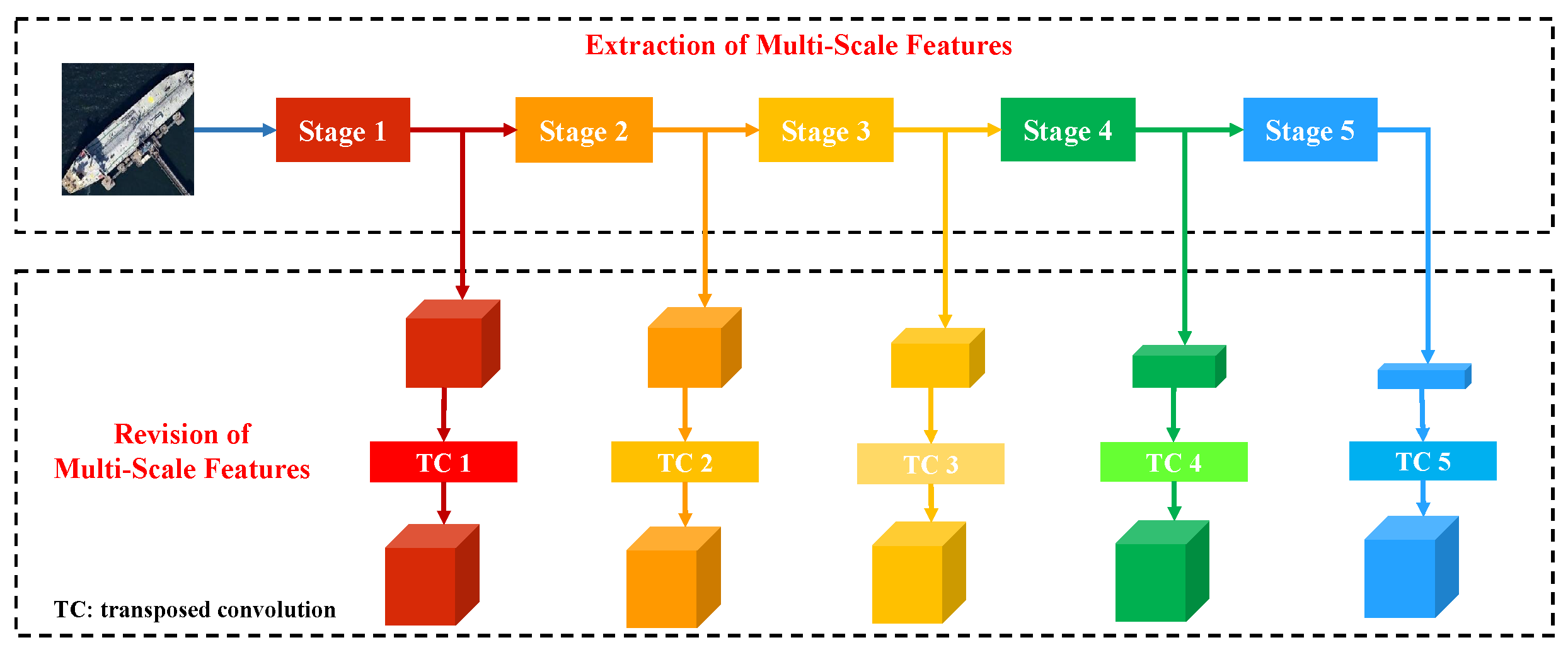
As mentioned above, the feature extractor used in this paper can be divided into five stages, namely, four convolution blocks and the last one average pooling block. Thus, we can combine these five stages to obtain multi-scale features. Considering that multi-scale fusion requires the consistency of dimensions, a transposed convolution operation is adopted to revise features of each stage to a certain extent. The structure of the extraction of multi-scale features is shown in Figure 3.
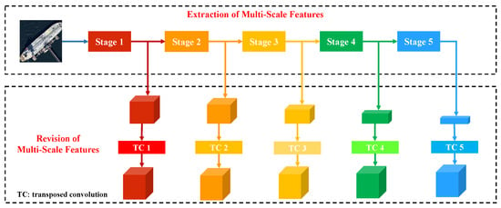
Figure 3.
The structure of the extraction of multi-scale features.
Therefore, for a remote sensing image , the extraction of multi-scale features can be defined as follows:
where denotes the extracted multi-scale features of the sample , represents the ith transposed convolution layer, stands for features output from the ith stage of the hidden layer, and the input image passes through the 1th, 2th, ⋯, and 5th stage of the hidden layers.
3.3. Construction of Graph-Based Features
In order to obtain more effective expression of the spatial information among remote sensing images, a construction model of graph-based feature is proposed based on the KNN algorithm, which can construct graph-based features to reflect relation information.
Assume the image features have the size of , where N expresses the batch size, C denotes the channel number of the feature, H and W, respectively, represent the height and the width of the feature. Graph-based features mainly include two types of features, one is node features and the other is edge features . In this paper, the feature of a whole graph is defined as follows:
where i represents the ith graph constructed by the ith scale image features, and .
Node features are essentially the denoted image features. More specifically, features of a node come from the features of an image obtained by the feature extractor. In our settings, batch norm is applied, which means N (batch size) images are imported at one time. Therefore, node features of a graph include features of N images. In our proposed model, features of different scales are considered, and all the node features in a graph are acquired at the same scale. Then the node features can be written as follows:
where , and represents the image features of the kth sample on the ith scale.
At the same time, we perform matrix transformation on the image features. The dimensions of features are transferred to , where T is equal to , which will not cause loss of information and aims to simplify the later calculation and programming.
The edge features reflect the degree of similarity among nodes, which are represented by an adjacent matrix . In order to obtain the adjacent matrix, cosine similarity between any two nodes is calculated firstly. For a certain node m, the cosine similarity can be calculated as follows:
where n denotes the sample index, and . Theoretically, we can calculate the distance between any two nodes. In order to reduce the model complexity, neighbor nodes are searched by KNN algorithm, where the most similar nodes are considered. For a certain node, the top k most similar nodes of the same class are represented, where the cosine similarity denotes the edge connection between them. Other nodes with much lower similarities are set to 0, which stands for no edge connection. Thus, the modified cosine similarity results with KNN algorithm can be denoted as .
Based on cosine similarity results, the adjacency matrix can be defined as follows:
Then, the adjacency matrix is normalized to yield the final adjacency matrix . The normalization process is represented as follows:
where stands for the degree diagonal matrix, and .
3.4. Fusion of Multi-Scale Graph-Based Features
To integrate different scale features, a fusion model of multi-scale graph-based features is developed to obtain more abundant and effective semantic information. The fusion model is considered from two perspectives, which are node features and edge features. With regard to node features, which are essentially image features, we can consider that features obtained from the deeper layers contain more abstract information, and, thus, the fusion weight should be larger for the deeper layers. At the same time, features from low-layer network include abundant detailed information, which should not be negligible. For scene classification, the proportion of low-layer features is relatively small, and, thus, the fusion weights of them are relatively lower.
As for edge features, they are constructed based on cosine similarity among node features. The edge feature can reflect the spatial relation between two nodes. Only when the cosine similarity of two nodes reaches a certain level, there can be a non-zero edge feature expression. The images of the same scene have the characteristics of high similarity information, even if there are some individual differences. Drawing on this assumption, we believe that after repeated training, features with high similarity extracted by the model are the key to classification and are worth retaining for feature fusion. The most straightforward way is to directly multiply the edge features and the node features, which can ignore the features of nodes that are not connected by edges.
Denoting the fused graph as , which includes the fused node features and the fused edge features . It can be defined as follows:
Based on the above analysis, the node features of five graphs with different scales are fused, where the fusion process is defined as follows:
where represents the identity matrix, and and stand for the hyper-parameters. In our framework, features of the fifth scale are obtained by the deepest layer, which means they contain the most effective information. is to enhance features of the fifth scale and fuse more effective information. is to weight graph-based features obtained from different scales to balance the importance of features from different levels. Here, features obtained from the deeper layer are corresponding to larger weight. Therefore, we set the rule that . is the degree to balance the neighbor information. The smaller the , the stronger the degree will be expressed.
After the node features are fused, the fused edge features are also constructed using the same method as above. The initial matrix based on the fused node features is generated as , and the corresponding degree diagonal matrix is denoted as . Thus, the standardized fused edge features are defined as follows
Finally, fused graph-based features of five scales are utilized for few-shot classification, where the logistic regression classifier is trained by and , and updated by . Labels of samples from are predicted to calculate classification accuracy.
4. Results
In this section, two public remote sensing datasets are applied to verify the effectiveness of the MGFF model. The datasets, parameter setting and experimental comparisons are presented in detail.
4.1. Datasets
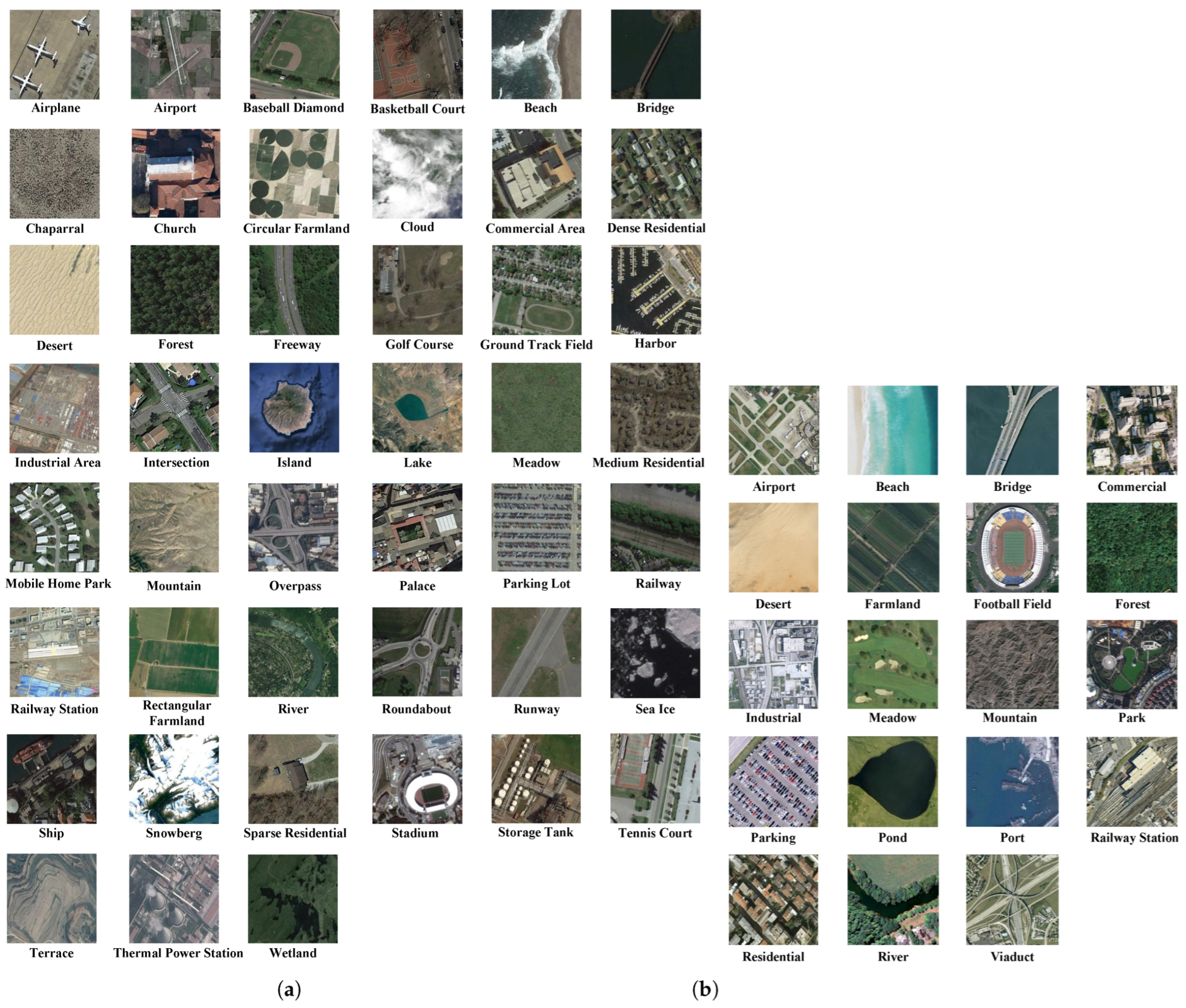
The evaluation of MGFF model is executed on two public available datasets, including NWPU-RESISC45 and WHU-RS19. These two datasets are depicted in Figure 4. NWPU-RESISC45 dataset [58] is a public dataset for remote sensing image scene classification, which was created by Northwestern Polytechnical University. This dataset consists of images with 45 categories, including airplane, chaparral, dense residential, forest, rectangular farmland, and so on. Each type consists of 700 images with pixels. In the evaluation experiments, 45 classes are divided into 25, 10, and 10 classes to, respectively, serve as the training set, validation set, as well as testing set. The details of data partitioning are reported in Table 1.
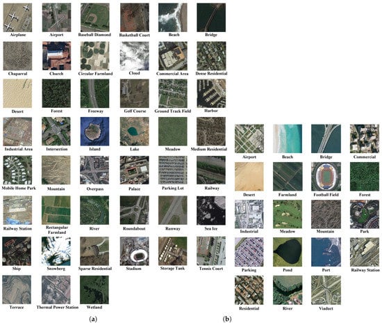
Figure 4.
Datasets utilized in the experiments, (a) images of NWPU-RESISC45 dataset, (b) images of WHU-RS19 dataset.

Table 1.
Details of NWPU-RESISC45 dataset and WHU-RS19 dataset.
WHU-RS19 dataset [59] is a benchmark for remote sensing image scene classification, which was established by Wuhan University. The dataset consists of 19 categories, including mountain, beach, park, commercial, farmland, railway station, desert, meadow, football field, industrial, forest, pond, parking lot, river, residential viaduct, port, bridge, and airport. Each category contains 50 or more images with pixels. In the evaluation experiments, 19 categories are divided into 9, 5, and 5 categories to serve as the training set, validation set, as well as testing set, respectively, which is shown in Table 1.
4.2. Experimental Settings
In our experiments, ResNet-12 is adopted as the backbone in our framework for feature extraction. In the pre-training stage, the weight factor of loss function is set to , and SGD optimizer is utilized as the optimization method. The learning rate is set to 0.001 and the batch size is set to 64. In order to construct graph-based features, the number of nodes in a graph should also be consistent with the batch size, which is set to 64. The settings of experiment parameters are summarized in Table 2. Other hyper-parameters are selected based on the experimental results, which have been discussed in the following subsection.

Table 2.
The settings of experiment parameters.
4.3. Comparisons with the State-of-the-Art Approaches
To verify the efficacy of the MGFF model, several state-of-the-art approaches for the same image scene classification task are applied for comparisons, including SCL-MLNet [60], Meta-SGD [61], TPN [62], Relation Net [41], MAML [63], DLA-MatchNet [48], and GES-Net [57]. In the field of few-shot scene classification of remote sensing images, the most concerned indicator is the overall classification accuracy. In order to compare fairly with other methods, we adopt the overall accuracy (ACC) as the evaluation index. In the experiments, classification results of 5-way 1-shot case and 5-way 5-shot case of each method are presented in Table 3 and Table 4, respectively.

Table 3.
Classification accuracies of 5-way 1-shot and 5-way 5-shot on the NWPU-RESISC45 dataset.

Table 4.
Classification accuracies of 5-way 1-shot and 5-way 5-shot on the WHU-RS19 dataset.
It can be clearly seen from Table 3 that our MGFF model produces the best accuracies under conditions of the two cases on NWPU-RESISC45 data, surpassing the GES-Net model by 4.26% and 0.97%, respectively. Compared with DLA-MatchNet, MGFF model has 6.29% and 1.61% improvements in 5-way 1-shot case and 5-way 5-shot case, respectively. Furthermore, the proposed MGFF is more advanced in terms of accuracy compared to the remaining other compared methods. It is verified that our proposed multi-scale graph-based feature fusion model is able to yield superb performance on NWPU-RESISC45 data.
Experimental comparisons conducted on WHU-RS19 dataset are shown in Table 4. Our proposed MGFF model presents the best results in cases of 5-way 1-shot and 5-way 5-shot. It exceeds the GES-Net model by 0.64% and 2.49%, respectively. Compared with DLA-MatchNet, MGFF model has 8.21% and 4.97% improvements under the two conditions. In addition, MGFF yields better few-shot classification performance contrast to other advanced approaches.
The above results illustrate that the proposed MGFF model is capable of effectively utilizing the limited information from a few samples, and through multi-scale graph-based feature fusion, information of the low-level features can be greatly reconciled with that of the high-level features. At the same time, our model excavates the spatial relations by construction of graph-based features from image features, so as to obtain more effective information than traditional methods. Therefore, the proposed MGFF is able to effectively ameliorate the accuracy of remote sensing image scene classification with limited labeled data.
In order to comprehensively present the classification effect of the proposed method, precision (PRE) and score () are also adopted as the evaluation indicators. The few-shot classification results of the proposed model are shown in the Table 5. It can be found that under two conditions, PRE and on the two datasets achieve excellent results close to ACC, which shows the effectiveness and stability of the proposed model.

Table 5.
Classification results of our proposed model on two datasets.
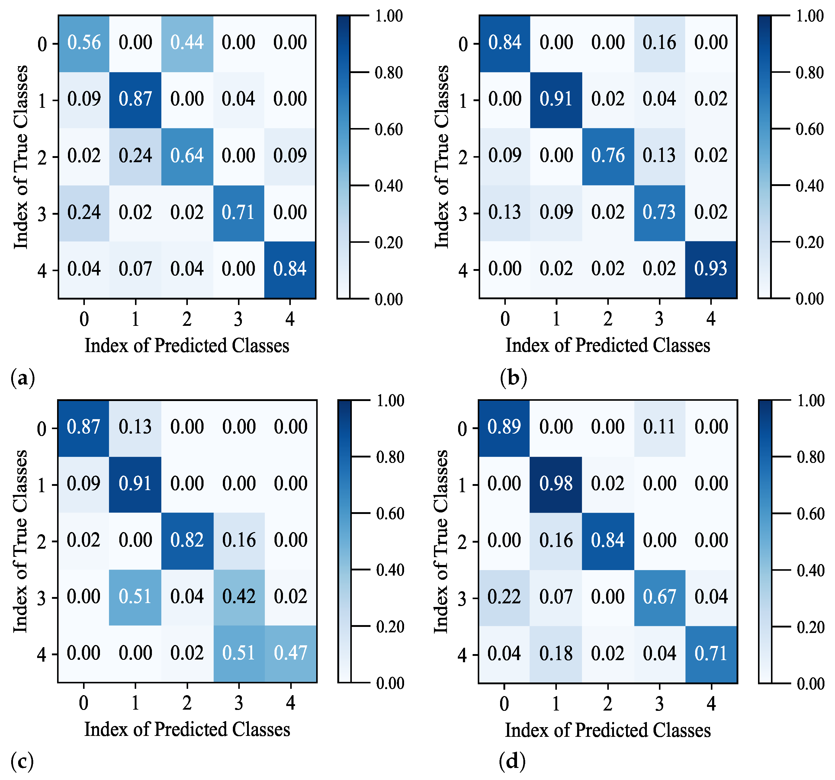
Moreover, similar to other literature [46,57], the confusion matrix is utilized to evaluate the performance of few-shot remote sensing image scene classification. Figure 5 shows the confusion matrices of the proposed model with different conditions on two datasets. It can be seen that performance of 5-way 5-shot is superior to that of 5-way 1-shot.
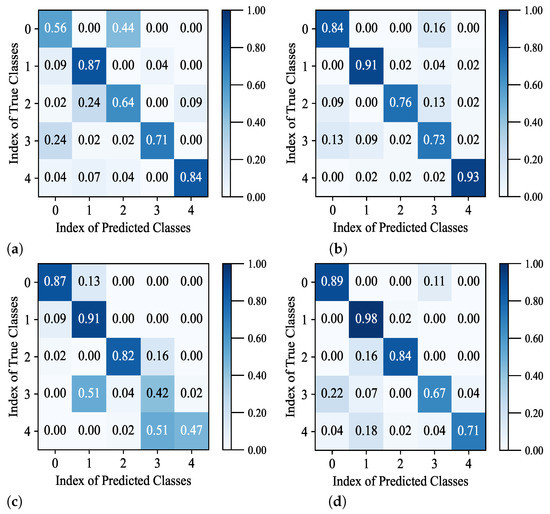
Figure 5.
Confusion matrices of our proposed model with different conditions on two datasets. (a) the confusion matrix on the NWPU-RESISC45 of 5-way 1-shot case, (b) the confusion matrix on the NWPU-RESISC45 of 5-way 5-shot case, (c) the confusion matrix on the WHU-RS19 of 5-way 1-shot case, and (d) the confusion matrix on the WHU-RS19 of 5-way 5-shot case.
5. Discussions
To further clearly discuss and illustrate the effectiveness of MGFF model, three kinds of ablation experiments are conducted, which are the effect of graph-based features, the effect of multi-scale feature fusion strategy and the effect of parameters.
5.1. Effect of Graph-Based Features
In our proposed model, in order to extract the spatial relation information, we construct graph-based features from the image features. To validate the effectiveness of this module, few-shot classification with or without graph-based features is conducted. In the comparisons, we perform linear weighted fusion of image features obtained from the feature extractor and transposed convolution layers. The compared results on NWPU-RESISC45 and WHU-RS19 are shown in Figure 6.
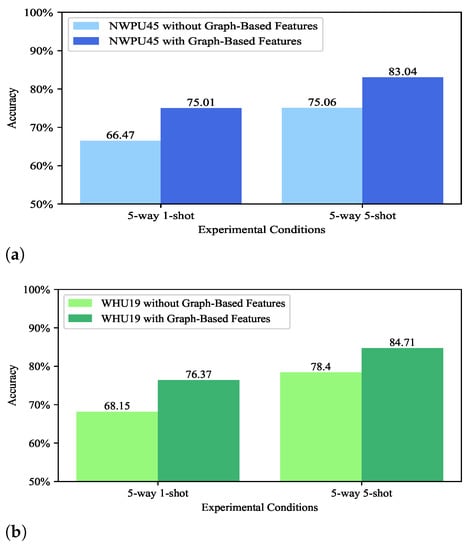
Figure 6.
Comparisons of different types of features on two datasets. (a) shows the test results on the NWPU-RESISC45 dataset with different types of features, (b) shows the test results on the WHU-RS19 dataset with different types of features.
It can be clearly seen from Figure 6, accuracy of the image feature fusion model is obviously lower than that of the graph-based feature fusion model. On the NWPU-RESISC45 dataset, under the two conditions, the accuracy results of the image feature fusion model are 66.47% and 75.06%, respectively, which are 8.54% and 7.98% lower than that of the graph feature fusion model. On the WHU-RS19 data, under the two conditions, the accuracy results of the image feature fusion model are 68.15% and 78.40%, respectively, which are 8.22% and 6.31% lower than that of the graph-based feature fusion model. It can be concluded that graph-based features reflect more effective information than image features, which have a significant effect on improving the accuracy of few-shot remote sensing image scene classification.
5.2. Effect of Multi-Scale Feature Fusion Strategy
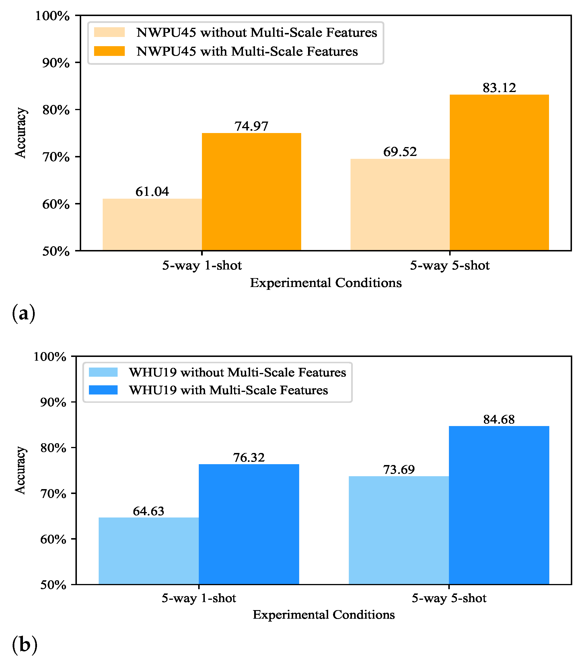
In MGFF model, a multi-scale graph-based feature fusion model is introduced to integrate high-level graph-based features with low-level graph-based features, where features of five different scales are fused. To illustrate the effectiveness of this fusion module, we conduct experiments on single-scale feature. In the compared model, the top-level features are obtained after five stages of the feature extractor, which is utilized for training and testing. Compared results obtained on NWPU-RESISC45 and WHU-RS19 are presented in the Figure 7.
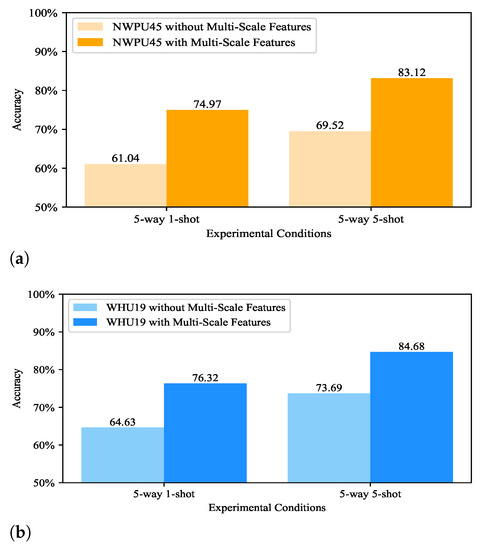
Figure 7.
Comparisons of different scales of features on two datasets. (a) shows the test results on the NWPU-RESISC45 dataset with different scales of features, (b) shows the test results on the WHU-RS19 dataset with different scales of features.
It can be clearly seen that without multi-scale feature fusion, the accuracy drops significantly. On the NWPU-RESISC45 dataset, under the two conditions, the accuracy results of the single-scale feature are 61.04% and 69.52%, respectively, which are 13.93% and 13.60% lower than that of the multi-scale feature fusion model. On the WHU-RS19 data, under the two conditions, the accuracies of the single-scale feature are 64.63% and 73.69%, respectively, which are 11.69% and 10.99% lower than that of the multi-scale feature fusion model, respectively. The compared results show that the multi-scale feature fusion model can make the features expressing specific information that the single-scale feature do not have, which is able to provide more effective knowledge for scene classification. Therefore, the developed multi-scale feature fusion strategy makes a great effect on boosting the accuracy of few-shot remote sensing scene classification.
5.3. Discussions of Parameters
In MGFF model, the parameters have great influence on the classification results. Thus, it is of great significance to analyze the parameters. There are mainly three types of hyperparameters in the proposed model, including parameters of graph-based feature construction model, parameters of multi-scale graph feature fusion, and parameters of the test condition.
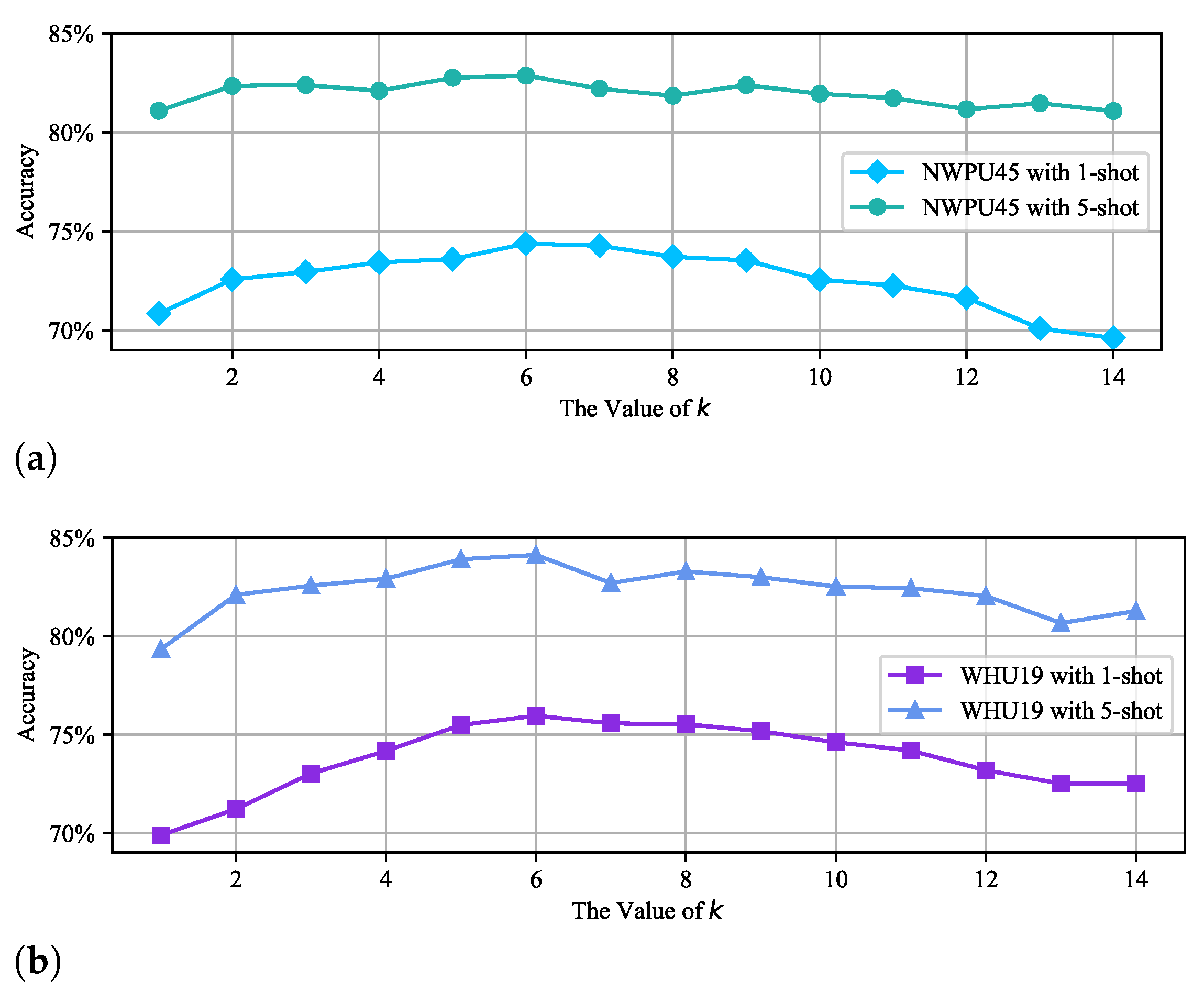
In our graph-based feature construction model, the hyperparameter k determines the number of connections between each node and other nodes in a single graph, which affects the expressiveness of edge features. So as to specifically illustrate the influence caused by the hyperparameter k to the final classification performance, we select a number of different values to conduct experiments under the condition of . The relevant experimental results are presented in the Figure 8, where k is changed from 1 to 14. It can be seen that the settings of different k will cause obvious differences in the classification accuracies, and the maximum difference of the accuracy changing can even reach about 6%. Furthermore, the classification performance will be achieved the best when k is set to 6.
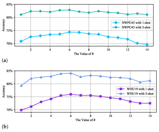
Figure 8.
Analysis with different values of k on two datasets. (a) shows the test results on the NWPU-RESISC45 dataset with different values of k, (b) shows the test results on the WHU-RS19 dataset with different values of k.
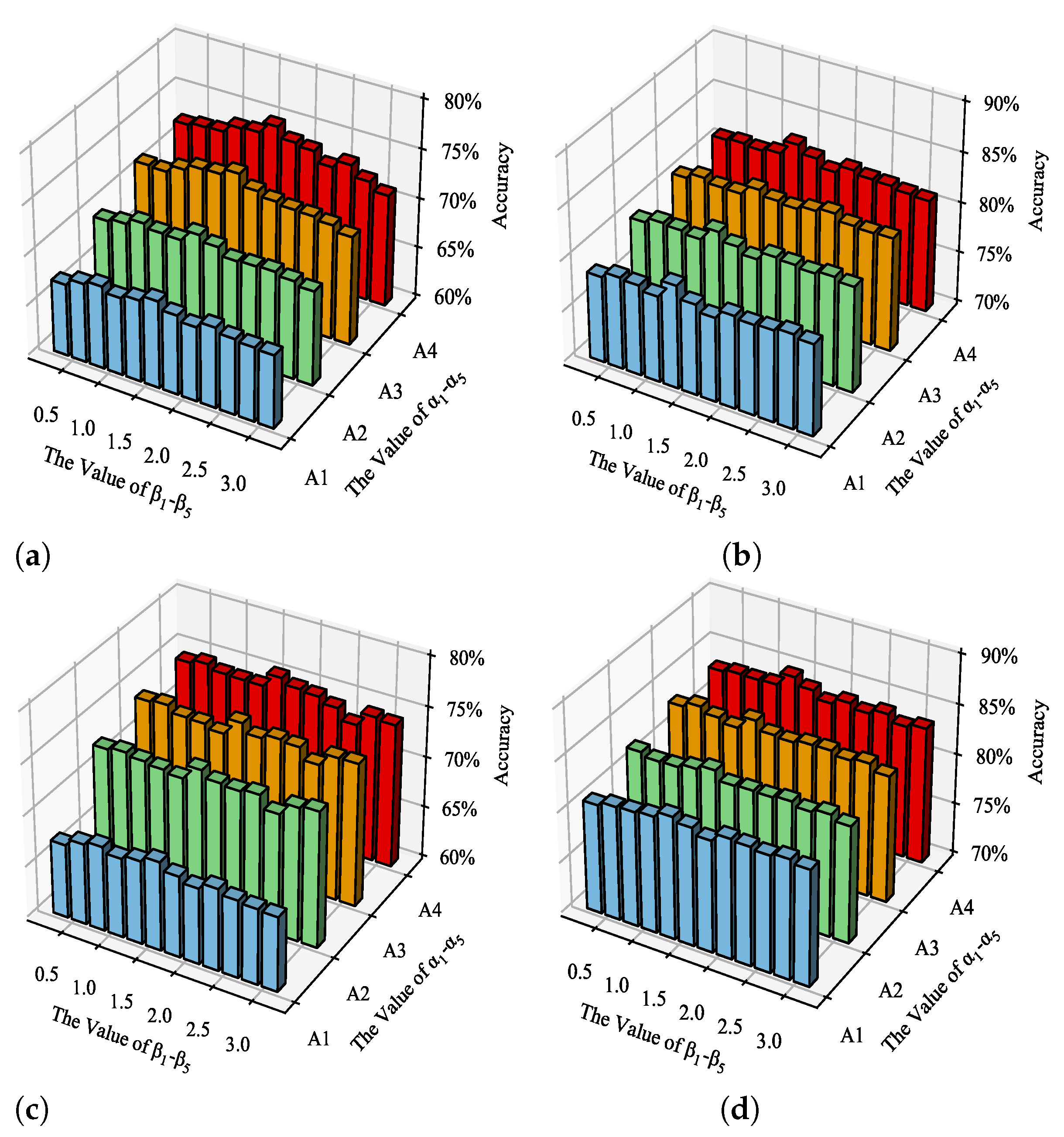
In our multi-scale graph-based feature fusion model, the fusion is conducted based on Equation (9), where there are multiple hyperparameters. These hyperparameters have a direct and important impact on the fusion of features. In order to explore the degree of their influence, we set four different groups of values for to , including A1( = 0.25, = 0.25, = 0.25, = 0.25, = 0.25), A2( = 0.20, = 0.20, = 0.20, = 0.20, = 0.25), A3( = 0.05, = 0.05, = 0.05, = 0.05, = 0.25), and A4( = 0.05, = 0.10, = 0.15, = 0.20, = 0.25). In addition, for to , we assume that they are all equal and set 12 different values ranging from to 3. Experimental results on NWPU-RESISC45 and WHU-RS19 are presented in Figure 9.
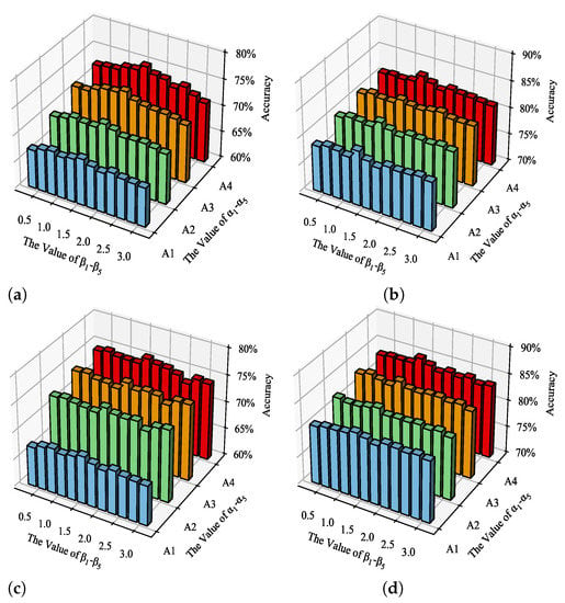
Figure 9.
Accuracy with different values of and on two datasets. (a,b) the results on the NWPU-RESISC45 under the condition of 5-way 1-shot and 5-way 5-shot, respectively. (c,d) the results on the WHU-RS19 under the condition of 5-way 1-shot and 5-way 5-shot, respectively.
It can be clearly seen from the Figure 9 that and make a great effect on the performance of the model. With different hyperparameter settings, the maximum impact on the accuracy can reach about 8%. For to , it is obvious that the weight setting of group A4 is optimal compared to the weight setting of other groups. The results verify that different hyperparameters should be set according to the scales of the graph-based features. For to , it is obvious the optimal parameter setting is . The results also show that a certain degree of exponentiation is beneficial to improve the classification results.
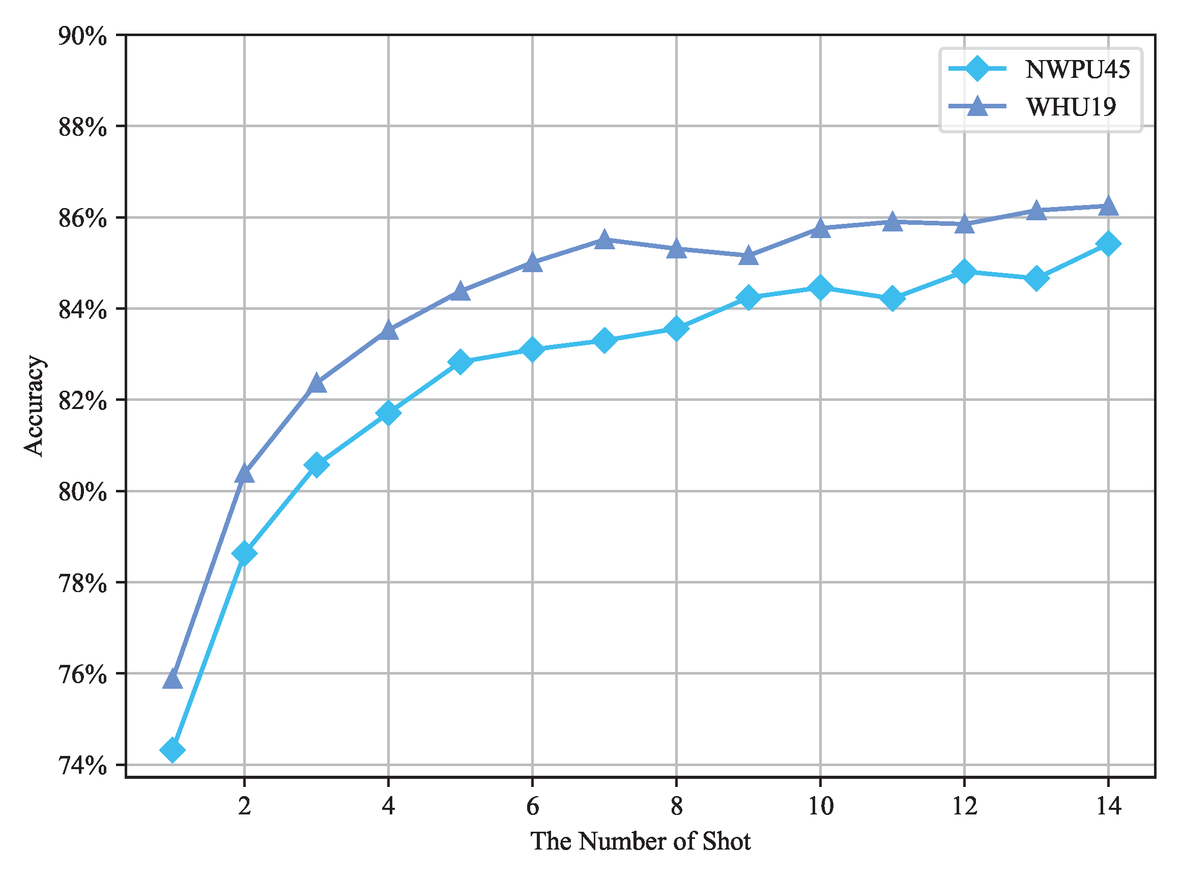
During the testing, the parameters of the test conditions can illustrate the accuracy of MGFF model on different cases. So as to explore the effect of the test conditions on the few-shot classification results, different numbers of shot are set for analysis, where the results on the two datasets are shown in the Figure 10.
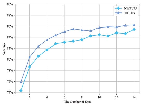
Figure 10.
Accuracy with different numbers of shot on two datasets.
From Figure 10, as the shot number increases, the accuracy of the proposed model on two datasets also increases. The growth rate is much faster when the shot number is lower than 5. When the shot number is greater than 5, the growth rate of the accuracy is gradually slowing down. Therefore, it is more appropriate for us to choose the number of 1 and 5 as the main test conditions, which, respectively, reflect the few-shot learning ability of MGFF model in the most extreme condition.
6. Conclusions
In this paper, a multi-scale graph-based feature fusion (MGFF) model is proposed for few-shot remote sensing image scene classification. In MGFF model, the graph-based feature learning is proved to take advantage of relation information for scene classification. Moreover, the graph-based feature fusion model is proposed to integrate graph-based features of multiple scales, which is verified to excavate more abundant semantic information and enhance sample discrimination. Experimental results on two public remote sensing datasets illustrate that the proposed MGFF method can achieve superior accuracy than other advanced few-shot scene classification approaches.
As for few-shot remote sensing image scene classification, there are still some issues worthy of further research. In the remote sensing data, there are still some noise data in the labeled samples. Therefore, it is an important research direction to establish a classification model with strong robustness that overcomes the influence of noise samples.
Author Contributions
Conceptualization, N.J. and J.G.; methodology, N.J. and J.G.; software, N.J. and H.S.; validation, N.J.; formal analysis, J.G.; investigation, N.J. and H.S.; data curation, N.J.; writing—original draft preparation, N.J., H.S. and J.G.; writing—review and editing, N.J., H.S. and J.G.; supervision, J.G. All authors have read and agreed to the published version of the manuscript.
Funding
This research was supported by National Natural Science Foundation of China under Grant 61901376, Project funded by China Postdoctoral Science Foundation under Grant 2021TQ0271 and Grant 2021M700110, and the national undergraduate innovation and entrepreneurship training program.
Institutional Review Board Statement
Not applicable.
Informed Consent Statement
Not applicable.
Data Availability Statement
The NWPU-RESISC45 dataset can be obtained from [58]. The WHU-RS19 dataset can be obtained from [59].
Conflicts of Interest
The authors declare no conflict of interest.
References
- Yao, X.; Han, J.; Cheng, G.; Qian, X.; Guo, L. Semantic annotation of high-resolution satellite images via weakly supervised learning. IEEE Trans. Geosci. Remote Sens. 2016, 54, 3660–3671. [Google Scholar] [CrossRef]
- Cui, Z.; Yang, W.; Chen, L.; Li, H. MKN: Metakernel networks for few shot remote sensing scene classification. IEEE Trans. Geosci. Remote Sens. 2022, 60, 1–11. [Google Scholar] [CrossRef]
- Zhao, B.; Zhong, Y.; Xia, G.S.; Zhang, L. Dirichlet-derived multiple topic scene classification model for high spatial resolution remote sensing imagery. IEEE Trans. Geosci. Remote Sens. 2015, 54, 2108–2123. [Google Scholar] [CrossRef]
- Huang, X.; Wang, Y. Investigating the effects of 3D urban morphology on the surface urban heat island effect in urban functional zones by using high-resolution remote sensing data: A case study of Wuhan, Central China. ISPRS J. Photogramm. Remote Sens. 2019, 152, 119–131. [Google Scholar] [CrossRef]
- Chen, S.W.; Cui, X.C.; Wang, X.S.; Xiao, S.P. Speckle-free SAR image ship detection. IEEE Trans. Image Process. 2021, 30, 5969–5983. [Google Scholar] [CrossRef]
- Xia, G.S.; Hu, J.; Hu, F.; Shi, B.; Bai, X.; Zhong, Y.; Zhang, L.; Lu, X. AID: A benchmark data set for performance evaluation of aerial scene classification. IEEE Trans. Geosci. Remote Sens. 2017, 55, 3965–3981. [Google Scholar] [CrossRef]
- Lowe, D.G. Distinctive image features from scale-invariant keypoints. Int. J. Comput. Vis. 2004, 60, 91–110. [Google Scholar] [CrossRef]
- Oliva, A.; Torralba, A. Modeling the shape of the scene: A holistic representation of the spatial envelope. Int. J. Comput. Vis. 2001, 42, 145–175. [Google Scholar] [CrossRef]
- Yang, Y.; Newsam, S. Bag-of-visual-words and spatial extensions for land-use classification. In Proceedings of the 18th SIGSPATIAL International Conference on Advances in Geographic Information Systems, Beijing, China, 2–5 November 2010; pp. 270–279. [Google Scholar]
- Shao, W.; Yang, W.; Xia, G.S. Extreme value theory-based calibration for the fusion of multiple features in high-resolution satellite scene classification. Int. J. Remote Sens. 2013, 34, 8588–8602. [Google Scholar] [CrossRef]
- Negrel, R.; Picard, D.; Gosselin, P.H. Evaluation of second-order visual features for land-use classification. In Proceedings of the 2014 12th International Workshop on Content-Based Multimedia Indexing (CBMI), Klagenfurt, Austria, 18–20 June 2014; IEEE: Piscataway, NJ, USA, 2014; pp. 1–5. [Google Scholar]
- Zhao, L.; Tang, P.; Huo, L. A 2-D wavelet decomposition-based bag-of-visual-words model for land-use scene classification. Int. J. Remote Sens. 2014, 35, 2296–2310. [Google Scholar] [CrossRef]
- Krizhevsky, A.; Sutskever, I.; Hinton, G.E. Imagenet classification with deep convolutional neural networks. Adv. Neural Inf. Process. Syst. 2012, 25. [Google Scholar] [CrossRef]
- Simonyan, K.; Zisserman, A. Very deep convolutional networks for large-scale image recognition. arXiv 2014, arXiv:1409.1556. [Google Scholar]
- Szegedy, C.; Liu, W.; Jia, Y.; Sermanet, P.; Reed, S.; Anguelov, D.; Erhan, D.; Vanhoucke, V.; Rabinovich, A. Going deeper with convolutions. In Proceedings of the IEEE Conference on Computer Vision and Pattern Recognition, Boston, MA, USA, 7–12 June 2015; pp. 1–9. [Google Scholar]
- Penatti, O.A.; Nogueira, K.; Dos Santos, J.A. Do deep features generalize from everyday objects to remote sensing and aerial scenes domains? In Proceedings of the IEEE Conference on Computer Vision and Pattern Recognition Workshops, Boston, MA, USA, 7–12 June 2015; pp. 44–51. [Google Scholar]
- Chen, S.W.; Tao, C.S. PolSAR image classification using polarimetric-feature-driven deep convolutional neural network. IEEE Geosci. Remote Sens. Lett. 2018, 15, 627–631. [Google Scholar] [CrossRef]
- Shawky, O.A.; Hagag, A.; El-Dahshan, E.S.A.; Ismail, M.A. Remote sensing image scene classification using CNN-MLP with data augmentation. Optik 2020, 221, 165356. [Google Scholar] [CrossRef]
- Zhang, T.; Liang, J.; Ding, B. Acoustic scene classification using deep CNN with fine-resolution feature. Expert Syst. Appl. 2020, 143, 113067. [Google Scholar] [CrossRef]
- Khan, A.; Chefranov, A.; Demirel, H. Image scene geometry recognition using low-level features fusion at multi-layer deep CNN. Neurocomputing 2021, 440, 111–126. [Google Scholar] [CrossRef]
- Mcilwaine, B.; Casado, M.R. JellyNet: The convolutional neural network jellyfish bloom detector. Int. J. Appl. Earth Obs. Geoinf. 2021, 97, 102279. [Google Scholar] [CrossRef]
- Gidaris, S.; Bursuc, A.; Komodakis, N.; Pérez, P.; Cord, M. Boosting few-shot visual learning with self-supervision. In Proceedings of the IEEE/CVF International Conference on Computer Vision, Seoul, Korea, 27 October–2 November 2019; pp. 8059–8068. [Google Scholar]
- Chu, W.H.; Li, Y.J.; Chang, J.C.; Wang, Y.C.F. Spot and learn: A maximum-entropy patch sampler for few-shot image classification. In Proceedings of the IEEE/CVF conference on Computer Vision and Pattern Recognition, Long Beach, CA, USA, 15–20 June 2019; pp. 6251–6260. [Google Scholar]
- Cheng, G.; Han, J.; Guo, L.; Liu, Z.; Bu, S.; Ren, J. Effective and efficient midlevel visual elements-oriented land-use classification using VHR remote sensing images. IEEE Trans. Geosci. Remote Sens. 2015, 53, 4238–4249. [Google Scholar] [CrossRef]
- Chen, S.W. SAR image speckle filtering with context covariance matrix formulation and similarity test. IEEE Trans. Image Process. 2020, 29, 6641–6654. [Google Scholar] [CrossRef]
- Wang, S.; Wang, X.; Zhang, L.; Zhong, Y. Auto-AD: Autonomous hyperspectral anomaly detection network based on fully convolutional autoencoder. IEEE Trans. Geosci. Remote Sens. 2021, 60, 1–14. [Google Scholar] [CrossRef]
- Zhu, S.; Du, B.; Zhang, L.; Li, X. Attention-based multiscale residual adaptation network for cross-scene classification. IEEE Trans. Geosci. Remote Sens. 2021, 60, 1–15. [Google Scholar] [CrossRef]
- Xu, C.; Zhu, G.; Shu, J. A lightweight and robust lie group-convolutional neural networks joint representation for remote sensing scene classification. IEEE Trans. Geosci. Remote Sens. 2021, 60, 1–15. [Google Scholar] [CrossRef]
- Wang, X.; Wang, S.; Ning, C.; Zhou, H. Enhanced feature pyramid network with deep semantic embedding for remote sensing scene classification. IEEE Trans. Geosci. Remote Sens. 2021, 59, 7918–7932. [Google Scholar] [CrossRef]
- Lu, X.; Zheng, X.; Yuan, Y. Remote sensing scene classification by unsupervised representation learning. IEEE Trans. Geosci. Remote Sens. 2017, 55, 5148–5157. [Google Scholar] [CrossRef]
- Cheng, G.; Xie, X.; Han, J.; Guo, L.; Xia, G.S. Remote sensing image scene classification meets deep learning: Challenges, methods, benchmarks, and opportunities. IEEE J. Sel. Top. Appl. Earth Obs. Remote Sens. 2020, 13, 3735–3756. [Google Scholar] [CrossRef]
- Lu, X.; Gong, T.; Zheng, X. Multisource compensation network for remote sensing cross-domain scene classification. IEEE Trans. Geosci. Remote Sens. 2019, 58, 2504–2515. [Google Scholar] [CrossRef]
- Nogueira, K.; Penatti, O.A.; Dos Santos, J.A. Towards better exploiting convolutional neural networks for remote sensing scene classification. Pattern Recognit. 2017, 61, 539–556. [Google Scholar] [CrossRef]
- Cheng, G.; Yang, C.; Yao, X.; Guo, L.; Han, J. When deep learning meets metric learning: Remote sensing image scene classification via learning discriminative CNNs. IEEE Trans. Geosci. Remote Sens. 2018, 56, 2811–2821. [Google Scholar] [CrossRef]
- Wang, Q.; Liu, S.; Chanussot, J.; Li, X. Scene classification with recurrent attention of VHR remote sensing images. IEEE Trans. Geosci. Remote Sens. 2018, 57, 1155–1167. [Google Scholar] [CrossRef]
- Tang, X.; Lin, W.; Ma, J.; Zhang, X.; Liu, F.; Jiao, L. Class-Level Prototype Guided Multiscale Feature Learning for Remote Sensing Scene Classification With Limited Labels. IEEE Trans. Geosci. Remote Sens. 2022, 60, 1–15. [Google Scholar] [CrossRef]
- Pires de Lima, R.; Marfurt, K. Convolutional neural network for remote-sensing scene classification: Transfer learning analysis. Remote Sens. 2019, 12, 86. [Google Scholar] [CrossRef]
- Zeng, Q.; Geng, J. Task-specific contrastive learning for few-shot remote sensing image scene classification. ISPRS J. Photogramm. Remote Sens. 2022, 191, 143–154. [Google Scholar] [CrossRef]
- Vinyals, O.; Blundell, C.; Lillicrap, T.; Wierstra, D. Matching networks for one shot learning. Adv. Neural Inf. Process. Syst. 2016, 29, 3637–3645. [Google Scholar]
- Snell, J.; Swersky, K.; Zemel, R. Prototypical networks for few-shot learning. Adv. Neural Inf. Process. Syst. 2017, 30, 4080–4090. [Google Scholar]
- Sung, F.; Yang, Y.; Zhang, L.; Xiang, T.; Torr, P.H.; Hospedales, T.M. Learning to compare: Relation network for few-shot learning. In Proceedings of the IEEE Conference on Computer Vision and Pattern Recognition, Salt Lake City, UT, USA, 18–23 June 2018; pp. 1199–1208. [Google Scholar]
- Zhang, X.; Qiang, Y.; Sung, F.; Yang, Y.; Hospedales, T. RelationNet2: Deep comparison network for few-shot learning. In Proceedings of the 2020 International Joint Conference on Neural Networks (IJCNN), Glasgow, UK, 19–24 July 2020; IEEE: Piscataway, NJ, USA, 2020; pp. 1–8. [Google Scholar]
- Alajaji, D.; Alhichri, H.S.; Ammour, N.; Alajlan, N. Few-shot learning for remote sensing scene classification. In Proceedings of the 2020 Mediterranean and Middle-East Geoscience and Remote Sensing Symposium (M2GARSS), Tunis, Tunisia, 9–11 March 2020; IEEE: Piscataway, NJ, USA, 2020; pp. 81–84. [Google Scholar]
- Jiang, W.; Huang, K.; Geng, J.; Deng, X. Multi-scale metric learning for few-shot learning. IEEE Trans. Circuits Syst. Video Technol. 2020, 31, 1091–1102. [Google Scholar] [CrossRef]
- Cheng, G.; Cai, L.; Lang, C.; Yao, X.; Chen, J.; Guo, L.; Han, J. SPNet: Siamese-prototype network for few-shot remote sensing image scene classification. IEEE Trans. Geosci. Remote Sens. 2021, 60, 1–11. [Google Scholar] [CrossRef]
- Zeng, Q.; Geng, J.; Jiang, W.; Huang, K.; Wang, Z. Idln: Iterative distribution learning network for few-shot remote sensing image scene classification. IEEE Geosci. Remote Sens. Lett. 2021, 19, 1–5. [Google Scholar] [CrossRef]
- Li, H.; Cui, Z.; Zhu, Z.; Chen, L.; Zhu, J.; Huang, H.; Tao, C. RS-MetaNet: Deep meta metric learning for few-shot remote sensing scene classification. arXiv 2020, arXiv:2009.13364. [Google Scholar] [CrossRef]
- Li, L.; Han, J.; Yao, X.; Cheng, G.; Guo, L. DLA-MatchNet for few-shot remote sensing image scene classification. IEEE Trans. Geosci. Remote Sens. 2020, 59, 7844–7853. [Google Scholar] [CrossRef]
- Zhai, M.; Liu, H.; Sun, F. Lifelong learning for scene recognition in remote sensing images. IEEE Geosci. Remote Sens. Lett. 2019, 16, 1472–1476. [Google Scholar] [CrossRef]
- Koch, G.; Zemel, R.; Salakhutdinov, R. Siamese neural networks for one-shot image recognition. In Proceedings of the ICML Deep Learning Workshop, Lille, France, 6–11 July 2015; Volume 2. [Google Scholar]
- Kim, J.; Kim, T.; Kim, S.; Yoo, C.D. Edge-labeling graph neural network for few-shot learning. In Proceedings of the IEEE/CVF Conference on Computer Vision and Pattern Recognition, Long Beach, CA, USA, 16–17 June 2019; pp. 11–20. [Google Scholar]
- Gidaris, S.; Komodakis, N. Generating classification weights with gnn denoising autoencoders for few-shot learning. In Proceedings of the IEEE/CVF Conference on Computer Vision and Pattern Recognition, Long Beach, CA, USA, 15–20 June 2019; pp. 21–30. [Google Scholar]
- Hamilton, W.L.; Ying, R.; Leskovec, J. Representation learning on graphs: Methods and applications. arXiv 2017, arXiv:1709.05584. [Google Scholar]
- Kipf, T.N.; Welling, M. Semi-supervised classification with graph convolutional networks. arXiv 2016, arXiv:1609.02907. [Google Scholar]
- Veličković, P.; Cucurull, G.; Casanova, A.; Romero, A.; Lio, P.; Bengio, Y. Graph attention networks. arXiv 2017, arXiv:1710.10903. [Google Scholar]
- Wu, F.; Souza, A.; Zhang, T.; Fifty, C.; Yu, T.; Weinberger, K. Simplifying graph convolutional networks. In Proceedings of the International Conference on Machine Learning, PMLR, Long Beach, CA, USA, 9–15 June 2019; pp. 6861–6871. [Google Scholar]
- Yuan, Z.; Huang, W.; Tang, C.; Yang, A.; Luo, X. Graph-Based Embedding Smoothing Network for Few-Shot Scene Classification of Remote Sensing Images. Remote Sens. 2022, 14, 1161. [Google Scholar] [CrossRef]
- Cheng, G.; Han, J.; Lu, X. Remote Sensing Image Scene Classification: Benchmark and State of the Art. Proc. IEEE 2017, 105, 1865–1883. [Google Scholar] [CrossRef]
- Sheng, G.; Yang, W.; Xu, T.; Sun, H. High-resolution satellite scene classification using a sparse coding based multiple feature combination. Int. J. Remote Sens. 2012, 33, 2395–2412. [Google Scholar] [CrossRef]
- Li, X.; Shi, D.; Diao, X.; Xu, H. SCL-MLNet: Boosting Few-Shot Remote Sensing Scene Classification via Self-Supervised Contrastive Learning. IEEE Trans. Geosci. Remote Sens. 2022, 60, 1–12. [Google Scholar] [CrossRef]
- Li, Z.; Zhou, F.; Chen, F.; Li, H. Meta-sgd: Learning to learn quickly for few-shot learning. arXiv 2017, arXiv:1707.09835. [Google Scholar]
- Liu, Y.; Lee, J.; Park, M.; Kim, S.; Yang, E.; Hwang, S.J.; Yang, Y. Learning to propagate labels: Transductive propagation network for few-shot learning. arXiv 2018, arXiv:1805.10002. [Google Scholar]
- Finn, C.; Abbeel, P.; Levine, S. Model-agnostic meta-learning for fast adaptation of deep networks. In Proceedings of the International Conference on Machine Learning, PMLR, Sydney, Australia, 6–11 August 2017; pp. 1126–1135. [Google Scholar]
Publisher’s Note: MDPI stays neutral with regard to jurisdictional claims in published maps and institutional affiliations. |
© 2022 by the authors. Licensee MDPI, Basel, Switzerland. This article is an open access article distributed under the terms and conditions of the Creative Commons Attribution (CC BY) license (https://creativecommons.org/licenses/by/4.0/).

