Abstract
Remote sensing nighttime lights (NTLs) offers a unique perspective on human activity, and NTL images are widely used in urbanization monitoring, light pollution, and other human-related research. As one of the payloads of sustainable development science Satellite-1 (SDGSAT-1), the Glimmer Imager (GI) provides a new multi-spectral, high-resolution, global coverage of NTL images. However, during the on-orbit testing of SDGSAT-1, a large number of stripes with bad or corrupted pixels were observed in the L1A GI image, which directly affected the accuracy and availability of data applications. Therefore, we propose a novel destriping algorithm based on anomaly detection and spectral similarity restoration (ADSSR) for the GI image. The ADSSR algorithm mainly consists of three parts: pretreatment, stripe detection, and stripe restoration. In the pretreatment, salt-pepper noise is suppressed by setting a minimum area threshold of the connected components. Then, during stripe detections, the valid pixel number sequence and the total pixel value sequence are analyzed to determine the location of stripes, and the abnormal pixels of each stripe are estimated by a clustering algorithm. Finally, a spectral-similarity-based method is adopted to restore all abnormal pixels of each stripe in the stripe restoration. In this paper, the ADSSR algorithm is compared with three representative destriping algorithms, and the robustness of the ADSSR algorithm is tested on different sizes of GI images. The results show that the ADSSR algorithm performs better than three representative destriping algorithms in terms of visual and quantitative indexes and still maintains outstanding performance and robustness in differently sized GI images.
1. Introduction
Ordinary remote sensing often uses land cover or land use changes to reflect human activities [1], such as deforestation [2,3,4] and target extraction [5,6]. With nighttime light (NTL) remote sensing gradually entering people’s view, the direct observation of artificial light from space is now a means of directly reflecting human activities, such as urbanization monitoring [7,8,9] and population and GDP estimations [10,11,12]. NTL remote sensing is also used to study the impact of light pollution on the ecological environment [13,14,15,16]. The Glimmer Imager (GI) is one of the payloads of sustainable development science Satellite-1 (SDGSAT-1), which has 40 m multispectral, 10 m panchromatic, and 300 km wide global NTL image acquisition capabilities [17,18]. Compared with existing easily accessible NTL images, GI images have advantages such as high resolutions, multi-spectrum, and large widths, which will further expand the application scene of NTL images, such as detecting and identifying different lights in a city and exploring the impact of different lights on human health [17]. On 21 September 2022, Chinese State Councilor and Foreign Minister Wang Yi announced the sharing of data obtained from the SDGSAT-1, launched by China in November 2021, with the rest of the world to help other countries with their research and policymaking regarding sustainable development at the Ministerial Meeting of the Group of Friends of the Global Development Initiative (GDI) on the sidelines of the ongoing UN General Assembly session in New York. This means that GI images are available for free. Thus, GI images will be one of the important supplements for existing NTL images. Table 1 shows some key parameters of GI images and other available NTL images.

Table 1.
Comparison of GI NTL data with other available data.
During the in-orbit testing of SDGSAT-1, many stripes with bad or corrupted pixels were observed in the L1A GI image (Figure 1). The existence of stripes will directly affect the quality of GI standard data products and the accuracy of further applications. Therefore, effectively restoring the stripes of the GI image is necessary. Previous destriping methods can be broadly divided into three categories: (1) statistics-based methods, (2) filtering-based methods, and (3) decomposition-model-based methods.

Figure 1.
A GI image (B1 band) with apparent stripes. The image has been processed by logarithmic stretching for better visualizations.
There are usually two ways of images destriping in statistics-based methods. One is based on the statistical characteristics of stripes. Stripes are first detected and then restored by interpolation. For instance, Han et al. found that the pixel value of stripes was lower than their left and right pixels in Hyperion images and labeled abnormal pixels based on this characteristic. The neighborhood averaging method was then applied to restore abnormal pixels [19]. The other is based on the statistical characteristics of the image, such as moment matching [20] and histogram matching [21]. However, when the statistical characteristics cannot accurately describe stripes, the effect of such methods is often unsatisfactory [22,23].
Filtering-based methods are generally divided into spatial filtering and frequency filtering. In the former, conventional spatial filters, such as the median filter, are simple to use and effective for restoring sparse stripes in the image. Nevertheless, these methods usually process all pixels in the image rather than those only in the stripe, which causes the image to lose a lot of information [24]. In the latter, Fourier or wavelet transformation is used to transform images into the frequency domain, and then the appropriate filter to suppress the stripe in the frequency domain is constructed, such as the Fourier domain filter [25], wavelet threshold [26,27], and both combined domain filters [28]. These methods perform well when stripes are distributed periodically in the image or can be distinguished easily in the power spectrum [29,30]. Similarly, the loss of information caused by the filter is inevitable.
The core idea of decomposition-model-based methods is that the original image consists of two parts: the stripe noise component and the clean image component. Then, the decomposition model is built with some regularization terms to separate the two components [31,32,33]. These methods have outstanding performances for optical, thermal infrared, and other traditional remote sensing images [31], such as the total variational model [33] and the low rank decomposition model [31,32]. However, fundamental to constructing such models is to accurately describe the characteristics of the stripe noise component and the clean image component. For example, in a low rank decomposition model, it is generally assumed that the rank of the matrix of the clean image component tends to be low or approximately low rank, and the stripe noise component can be separated by approximating the clean image components with a low-rank matrix. Therefore, the performance of these methods is unsatisfactory in images that do not conform to the hypothesis.
Previous destriping algorithms have rarely been applied to NTL images, and GI images are vastly different from other types of remote sensing images. Therefore, previous destriping algorithms may not be suitable for GI images, and we proposed a destriping algorithm for GI images based on anomaly detection and spectral similarity restoration (ADSSR). The ADSSR algorithm consists of three parts: pretreatment, stripe detection, and stripe restoration. In the pretreatment, the salt-pepper noise is suppressed by the connected component analysis. During stripe detections, we analyze the valid pixel number sequence and the total pixel value sequence to determine the location of stripes, and then we obtain the abnormal pixels of each stripe using a clustering algorithm. Finally, in the stripe restoration, we use the spectral similarity between abnormal pixels and neighboring pixels to restore abnormal pixels. The experiments on different sizes of GI images demonstrate that the ADSSR algorithm has outstanding performances for GI image destriping. In other words, it not only effectively detects and restores stripes but also retains most information. Moreover, the main contributions of this paper are summarized as follows:
- The characteristics of the stripe are analyzed and summarized. The bright stripe factor sequence (BSFS) and the dark stripe factor sequence (DSFS) are defined to locate the bright stripe and the dark stripe in the GI image, respectively.
- A spectral-similarity-based method is introduced to restore the stripe in the GI image, which considers the spectral similarity between pixels and has a better restoring effect of the stripe in the GI image compared with other restoration methods.
- The ADSSR algorithm is proposed to effectively restore stripes for the GI image, which provides a feasible method to improve the quality of the GI image.
- The residual noise entropy (RNE) is defined to quantify the destriping performance, which provides a new quantitative evaluator for destriping the GI image.
The remainder of this paper is organized as follows. In Section 2, the characteristics of GI images and stripes are analyzed in detail. Section 3 describes the basic process of the ADSSR algorithm. Two experiments are designed for evaluating the performance of the ADSSR algorithm and the corresponding results are presented in Section 4. Section 5 states the applicable scope of the proposed ADSSR algorithm and some problems that require improvements, and Section 6 is the conclusion.
2. Data Analysis
Compared with other types of remote sensing images, GI images are vastly different. Therefore, it is necessary to analyze the characteristics of images and stripes before introducing the ADSSR algorithm.
2.1. Image Characteristics Analysis
NTL images are usually acquired at night and mainly record light information in urban areas. Mountains, wilderness, and other unlit areas often have no information on NTL images. In L1A GI images, the pixel value of the unlit area is recorded as 0, which means that informative pixels can be distinguished by this value. Usually, the unlit area reaches very high proportions in GI images. For example, the pixel number of the unlit area reaches 82.47% of the GI image shown in Figure 2a. In addition, as shown in Figure 2b, the pixel value distribution of the image is extremely uneven, especially in urban areas. The pixel values of commercial areas and roads are significantly higher than those of residential areas. This results in a very low contrast in GI images without stretching. In order to better display GI images in this article, we used logarithmic stretching, as shown in Equation (1), to enhance image contrasts:
where represents the matrix of the raw image, and stands for the matrix of the contrast enhanced image. It is easy to observe that the contrast-enhanced image has a better display effect in Figure 2.
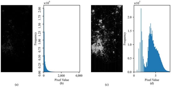
Figure 2.
Comparison before and after image contrast enhancement. (a) Raw image; (b) the histogram of raw image; (c) contrast enhanced image; (d) the histogram of contrast enhanced image. The frequency of 0 is too high, which will affect the readability of the histogram, and we ignored 0 when drawing the histogram.
2.2. Stripes Characteristics Analysis
As shown in Figure 3, the stripe of GI images mainly appears along the column. According to the visual characteristics, the stripe is divided into two types: (1) the bright stripe and (2) the dark stripe.
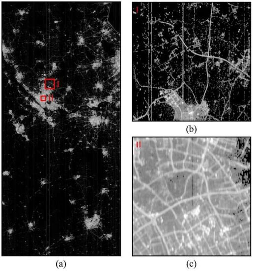
Figure 3.
Different types of stripes in GI images (B1 Band). (a) Full-size image; (b) bright stripes; (c) dark stripes.
- (1)
- The bright stripe
The bright stripe appears along the column independently or continuously, and the continuity of the stripe is also random. The pixel value of the bright stripe is not constant but variable and usually greater than that of its two sides. Moreover the bright stripe is the most common type of stripe in the GI image.
- (2)
- The dark stripe
Different from the bright stripe, the dark stripe only appears in artificial light areas. The column number of the dark stripe is still random. The dark stripe is intermittent. The pixel value of the dark stripe is also variable and usually lower than that of its two sides. Compared with the bright stripe, the dark stripe appears relatively infrequently in the image.
3. Methods
As shown in Figure 4, the ADSSR algorithm is mainly composed of three parts: the first part is to preprocess the image and suppress salt-pepper noise in the image; the second part is to detect the bright and dark stripes in the image; the third part is to restore the stripes in the image based on the spectral similarity. The details of the three parts are presented in Section 3.1, Section 3.2, and Section 3.3, respectively.
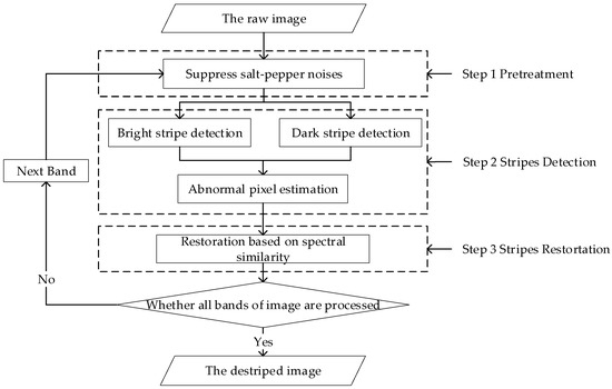
Figure 4.
The flowchart of the ADSSR algorithm.
3.1. Pretreatment
In Figure 1 and Figure 3, we can observe the salt-pepper noise except for the stripe noise in the original image, which also affects the image’s quality. In pretreatment, the main purpose is to suppress the salt-pepper noise. The salt-pepper noise can be regarded as many independent connected components with a small area based on image morphology. Therefore, the salt-pepper noise is suppressed based on this characteristic. First of all, the original image is converted into a binary image with 0 as the threshold. Then, the connected components of the original image are calculated based on 8 connected domains. Then, a minimum area threshold is set for the connected components, and if the area of the connected components is lower than the threshold, it will be labeled as salt-pepper noise. Finally, the salt-pepper noise is suppressed by using mask treatments. The steps of the salt-pepper noise suppression algorithm are as shown in Algorithm 1, and variable names that appear in the algorithm are bolded in italics.
| Algorithm 1. Salt-pepper noise suppression |
| Input: SDGSAT-1 GI original image original_img |
| 1: Transform original_img into a binary image with 0 as the threshold binary_img 2: Calculate the connected component of binary_img connected_component_set 3: Set the minimum area threshold of connected_component th 4: for connected_component in connected_component_set: 5: Calculate the area of connected_component tmp_area 6: if tmp_area < th: 7: connected_component is labeled as the salt-pepper noises 8: All labeled connected_component constitute the salt-pepper noise mask 9: Mask treatment to filter salt-pepper noise of original_img Output: SDGSAT-1 GI preprocessed image pre_img |
3.2. Stripe Detection
In GI images, the pixel with a value greater than 0 is defined as the valid pixel. We designed corresponding detection algorithms based on the characteristics of bright and dark stripes described in Section 2.2.
3.2.1. Bright Stripe Detection
For the bright stripe detection, it is noteworthy that the valid pixel number of the stripe is much higher than that in the column without stripes (Figure 5). Therefore, it provides an idea for locating the bright stripe by detecting the anomaly in the valid pixel number along the column.
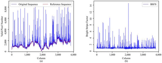
Figure 5.
The bright stripe detection of the image shown in Figure 3a. (a) The valid pixel number sequence; (b) the bright stripe factor sequence.
Firstly, 0 is used as the threshold to convert the original image to a binary image, and an original sequence that records the valid pixel number is obtained by summing each column of the binary image. Then, median smoothing is applied to this sequence to obtain a reference sequence without the stripe information. In order to detect anomalies in the original sequence, the bright stripe factor sequence (BSFS) is defined as shown in Equation (2):
where denotes the original sequence, and represents the reference sequence. is a constant that prevents the denominator from being 0. Based on BSFS and the original sequence, the column of the bright stripe is marked with two conditions. In the column where the bright stripe appears, the valid pixel number should be greater than a user-defined threshold, and the bright stripe factor should be greater than another user-defined threshold. As shown in Algorithm 2, the process of the bright stripe detection is listed, and variable names that appear in the algorithm are bolded in italics.
| Algorithm 2. Bright stripe detection |
| Input: SDGSAT-1 GI preprocessed image pre_img |
| 1: Convert pre_img into a binary image with 0 as the threshold binary_img 2: Sum each column of binary_img to get an original sequence original_seq 3: Set the median smoothing step size ms_step 4: reference_seq = median(original_seq, ms_step) 5: BSFS = original_seq/(reference_seq + 1) 6: Set the threshold of the valid pixel number, and the threshold of the bright stripe factor. th1, th2 7: Calculate the column number N of binary_img 8: Create an empty list bs_col_list to record the column index of the bright stripe 9: for i in range(N): 10: if original_seq[i] > th1 and BSFS[i] > th2: 11: bs_col_list.append(i) Output: The column index list of the bright stripe bs_col_list |
3.2.2. Dark Stripe Detection
In contrast to the bright stripe, it is difficult to locate the dark stripe by analyzing the valid pixel number sequence. However, considering the characteristics of the dark stripe in Section 2.2, the total pixel value of the column where the dark stripe appears is much lower than that of the neighboring column (Figure 6).
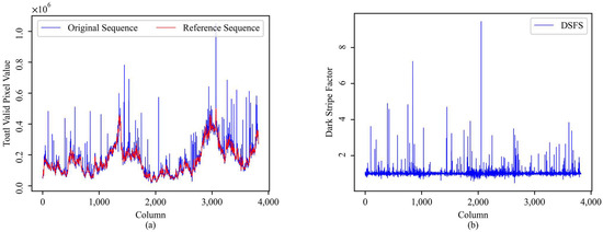
Figure 6.
The dark stripe detection of the image shown in Figure 3a. (a) The total pixel value sequence; (b) the dark stripe factor sequence.
Thus, we sum each column of the original image and obtain the total pixel value sequence. Similarly, we apply median smoothing to the total pixel value sequence to simulate a reference sequence without the stripe information. Then, we define the dark stripe factor sequence (DSFS) as shown in Equation (3):
where is the total pixel value sequence, and indicates the reference sequence. stands for a constant that prevents the denominator from being 0. Finally, the column is labeled as a dark stripe, when the number of valid pixels is greater than a user-defined-threshold and the dark stripe factor is less than another user-defined-threshold. Moreover, Algorithm 3 shows the basic steps of the dark stripe’s detection, and variable names that appear in the algorithm are bolded in italics.
| Algorithm 3. Dark stripe detection |
| Input: SDGSAT-1 GI preprocessed image pre_img |
| 1: Sum each column of pre_img to obtain an original sequence original_seq 2: Set the median smoothing step size ms_step 3: reference_seq = median(original_seq, ms_step) 4: DSFS = original_seq/(reference_seq + 1) 5: Set the threshold of the valid pixel number, and the threshold of the dark stripe factor. th1, th2 6: Calculate the column number N of pre_img 7: Create an empty list ds_col_list to record the column index of the dark stripe 8: for i in range(N): 9: Calculate the valid pixel number ni in column i 10: if ni > th1 and DSFS[i] < th2: 11: bs_col_list.append(i) Output: The column index list of the dark stripe ds_col_list |
3.2.3. Abnormal Pixel Estimation
Since there are intermittent stripes in the bright and dark stripes, it would be illogical to directly restore all pixels in the stripes. It is necessary to estimate the abnormal pixels that need to be restored in the stripes. First and foremost, the characteristics of the abnormal pixels in the stripe are analyzed. As shown in Figure 7, although the values of abnormal pixels are variable, they are approximately a stationary sequence. It is assumed that the fluctuation of the stationary sequence along the mean value follows the normal distribution, and Equation (4) can be used to locate abnormal pixels. All pixels of the stripe are traversed, and if the pixel value is less than the threshold in Equation (4), it is labeled as an abnormal pixel. The steps of abnormal pixel estimation are listed in Algorithm 4, and variable names that appear in the algorithm are bolded in italics..
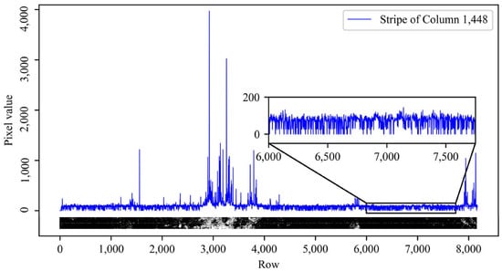
Figure 7.
The pixel value sequence of the stripe. The stripe appears in column 1448 of the image shown in Figure 3a.
Here, represents the threshold to identify abnormal pixels, and denotes the stationary sequence consisting of abnormal pixel values. and are the mean and the standard deviation of , respectively.
| Algorithm 4. Abnormal pixel estimation |
| Input: The column vector of the stripe stripe_vector |
| 1: Estimate the stationary sequence S_sta based on DBSCAN algorithm [34] 2: Calculate the threshold to identify abnormal pixels T_est by Equation (4) 3: Calculate the length L of stripe_vector 4: Create an empty list ap_row_list to record the row index of abnormal pixels 5: for i in range(L): 5: if stripe_vector[i]<T_est: 6 ap_row_list.append(i) Output: The row index list of abnormal pixels ap_row_list |
3.3. Stripe Restoration
The neighborhood averaging method is usually used to restore stripes after detecting bright and dark stripes and identifying the abnormal pixels in each stripe. However, this method relies heavily on the similarity of the neighboring pixels and will lead to a large error when the similarity of the neighboring pixels is poor [8,23].
Therefore, a restoration method based on spectral similarity has been adopted [23]. As shown in Figure 8, the multispectral image is a data cube composed of three bands. The spectral vector corresponding to each pixel can be defined as the form of S(s1, s2, s3), where s1, s2, and s3 stand for the pixel value in band 1, band 2, and band 3, respectively. We assume that band 1 is the band that needs to be restored in Figure 8. First, judging whether the left and right sides of the unrestored stripe are still stripes, if the left column is a stripe, add the column number until it is not a stripe, and for the right column, decrease the column number until it is not a stripe. The final two columns are regarded as reference data. Secondly, for each abnormal pixel in the stripes, the six nearest pixels are selected from the reference data. The spectral vectors corresponding to the abnormal pixel and the nearest pixels can be written as A(a1, a2, a3) and N(n1, n2, n3), respectively. Then, the Euclidean distance is used to evaluate the spectral similarity between the abnormal pixel and the nearest pixels. Because band 1 is unrestored, we only consider the second and third components when calculating the Euclidean distance, as shown in Equation (5):
where represents the Euclidean distance between the abnormal pixel and the nearest pixel, stands for the spectral vector corresponding to the abnormal pixel, and denotes the spectral vector corresponding to the nearest pixel. The smaller the distance, the higher the spectral similarity. Finally, in the six nearest pixels, the n1 of the nearest pixel that has the highest spectral similarity is used to replace the a1 of the abnormal pixel. Algorithm 5 provides the complete steps of stripe restoration, and variable names that appear in the algorithm are bolded in italics.
| Algorithm 5. Stripe restoration. |
| Input: The multispectral image ms_img |
| 1: Suppress the salt-pepper noise by Algorithm 1 pre_ms_img 2: Assume band 1 of pre_ms_img is unrestored 3: b1_img = pre_ms_img[:,:,0], b2_img = pre_ms_img[:,:,1], b3_img = pre_ms_img[:,:,2] 4: Obtain the column index list of bright stripes bs_col_list in b1_img by Algorithm 2 5: Obtain the column index list of dark stripes ds_col_list in b1_img by Algorithm 3 6: Merge bs_col_list and ds_col_list stripe_col_list 7: for col in stripe_col_list: 8: s_vector =b1_img[:,col] 9: Obtain the row index list of abnormal pixels ap_row_list by Algorithm 4 10: left_col = col + 1 11: right_col = col−1 12: while(left_col in stripe_col_list): 13: left_col = left_col + 1 14: while(right_col in stripe_col_list): 15: right_col = right_col + 1 16: ref_data = hstack(pre_ms_img[:,left_col,:], pre_ms_img[:,right,:]) 17: for row in ap_row_list: 18: ap_ spectral_vector =pre_ms_img[row,col,:] 19: ns_spectral_vector_set = ref_data[row−1:row + 2,:,:] 20: Initial i0 = 0, j0 = 0, d0 = 10e6 20: for i in range(2): 21: for j in range(3): 22: ns_spectral_vector = ns_spectral_vector_set[i,j,:] 23: Calculate the Euclidean distance tmp_d by Equation (5) 25: if tmp_d < d0: 26: d0 = tmp_d, i0 = i, j0 = j 27: pre_ms_img[row,col,0] = ns_spectral_vector_set[i0,j0,0] Output: b1_img with stripe restoration |
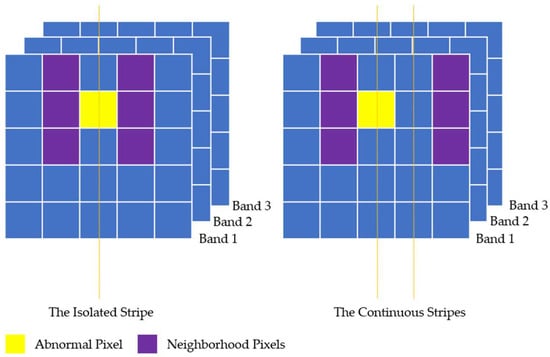
Figure 8.
Abnormal pixel restoration schematic diagram. The yellow pixel represents the abnormal pixel, the purple pixel stands for the neighborhood pixel, and the blue pixel denotes unselected pixel in this restoration.
4. Experiment and Results
Two experiments are designed to verify the effectiveness and performance of the ADSSR algorithm. The first experiment is used to compare the performance of the ADSSR algorithm with three representative algorithms, and the second experiment is mainly used to test the robustness of the proposed algorithm for the full-size GI image. All experiments are conducted under Windows 10 with an Intel (R) Core (TM) i5-9500 CPU at 3.00 GHz and 16 GB of memory. ADSSR algorithms are implemented using the Python language, and the parameters of the ADSSR algorithm used in all image processing are the same. There are five main parameters in the ADSSR algorithm. The minimum area threshold in Algorithm 1 is set as 8; the valid pixel number threshold in Algorithms 2 and 3 is set as the number of image lines multiplied by 0.125; the bright stripe factor threshold in Algorithm 2 is set as 1.35; the dark stripe factor threshold in Algorithm 3 is set as 0.75.
The details of two experiments are described in Section 4.1, and the results are presented in Section 4.2. Besides the subjective visual evaluation, the objective quantitative evaluation is also necessary. Due to the lack of the noiseless GI image, the peak signal-to-noise ratio (PSNR) and the structural similarity index (SSIM) are not suitable for evaluating image quality. Considering that the area without artificial light in the GI image usually only contains noise, the residual noise entropy (RNE) is defined to quantify the destriping performance of the methods. It can be calculated by using Equation (6):
where i represents the pixel value, n is the maximum pixel value, and Pi denotes the proportion of the pixel value i. RNE is calculated for one 10 × 10 pixels area that only contains noise in the GI image. Ideally, all noise is removed after processing, and the corresponding RNE is 0. In other words, the lower the RNE, the better the destriping performance.
In addition, the mean relative deviation (MRD), another quality index without reference, is also adopted to evaluate the effect of all destriping methods on the area that is less affected by the stripe noise or no stripes. The MRD is defined as Equation (7):
where represents the pixel value of the original subimage in row i and column j, stands for the pixel value of the destriped subimage in row i and column j, and m and n are the number of rows and columns of the subimage. It is noteworthy that the lower the MRD, the smaller the information loss of the destriped image.
4.1. Experiments Details
4.1.1. Comparative Experiment
Six test images were used for this experiment. Each image has 2000 × 2000 pixels and is acquired from different regions. The detailed information of all test images is shown in Figure 9 and Table 2. Moreover, we selected three representative algorithms for comparative experiments with the ADSSR algorithm: the low-rank tensor decomposition (LRTD) algorithm [32], the 1-D-guided filtering (GF) algorithm [35], and the wavelet threshold (WT) algorithm [36,37].
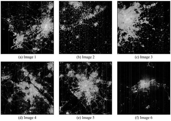
Figure 9.
Six test images. (a–f) All test images have been processed by logarithmic stretching for better visualization.
Table 2.
The detailed information of six test images.
4.1.2. Full-Size Images Experiment
In order to better test the robustness of the proposed algorithm, it was applied to two full-size GI images. Table 3 shows the detailed information of two full-size GI images in this experiment.
Table 3.
The detailed information of two full-size images.
4.2. Experiments Results
4.2.1. Results of Comparative Experiment
Figure 10 shows the results of different destriping algorithms. Compared with the original image, it can be found that the ADSSR algorithm can effectively remove most of the stripes and improve the visual quality of all the test images. In addition, there are almost no residual stripes left. The performance of LRTD is erratic. For Image 2, LRTD can also remove most of the stripes with a few residual stripes. However, in the other five test images, LRTD performed poorly, and the residual stripes are apparent. GF and WT not only failed to remove the stripes but also introduced new noise in all test images. The main reason is that the filters used in GF and WT are applied to the entire image, which will make the gray distribution of the entire image more uniform. This results in the poorer quality of filtered images, as the gray distribution of the GI image itself is extremely uneven. RNE and MRD for all images in Figure 10 are calculated and listed in Table 4, in which the best results are highlighted in bold and the second best are underlined. Compared with LRTD, GF, and WT, it can be seen that the ADSSR algorithm achieves the lowest RNE and MRD in all test images. Because the ADSSR algorithm only restores columns with stripes, the MRD calculation results are consistent and very close to the original image. The lowest RNE and the lowest MRD indicate minimal residual noise and minimal information loss, respectively. Therefore, both visually and quantitatively, the ADSSR algorithm has better performance than the other compared algorithms.
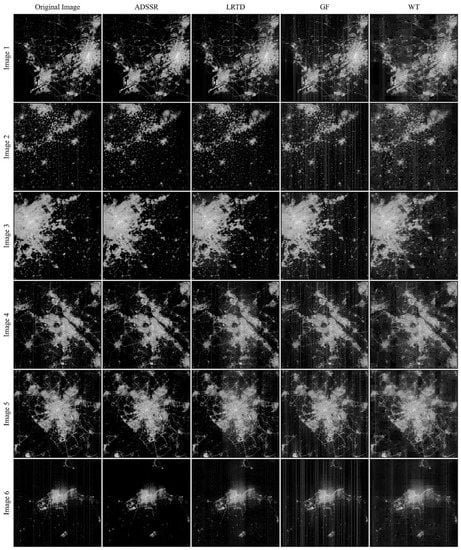
Figure 10.
Destriping results of six test images.
Table 4.
Performance comparison of all competing algorithm.
4.2.2. Results of Full-Size Images Experiment
As shown in Figure 11, it can be seen that the ADSSR algorithm can effectively remove most of stripes while maintaining a few residual stripes on two full-size images. In addition, the ADSSR algorithm almost prevents the information loss of the city area in the window scaling image. Moreover, the quantitative indexes are shown in Table 5, and in which the best results are highlighted in bold. The RNE values of the destriped images are significantly lower than the original image, and the MRD values of the destriped images are 0. This indicates that the proposed ADSSR algorithm can effectively remove stripes without damaging the original image information nearly, which is consistent with the visual conclusion.
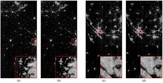
Figure 11.
Destriping results of two full-size images. (a) Original Image 1. (b) Destriped Image 1. (c) Original Image 2. (d) Destriped Image 2. (a–d) All images have been processed by logarithmic stretching for better visualizations.
Table 5.
Quantitative indicators of full-size image experiments.
5. Discussion
Some problems and the applicable scope of the ADSSR algorithm are discussed and analyzed in this section.
The ADSSR algorithm can be divided into three parts: pretreatment, stripe detection, and restoration. During stripe detection, as a good background value, 0 in the GI image provides a guarantee for determining the stripe’s location by analyzing the valid pixel number sequence and the total pixel value sequence. At the same time, the pixel value of the abnormal pixels in the stripes should be approximately stationary or follow the normal distribution so as to ensure that the outlier detection can effectively filter out normal pixels to locate abnormal pixels before the stripe’s restoration. Moreover, during stripe restoration, there are various methods, and the most common is the neighborhood averaging method. However, the method based on spectral similarities adopted in this paper has a better effect on image detail restorations, as shown in Figure 12. Stripes can be restored by these methods, which also depend on the fact that the stripes in the GI image are sparse. Therefore, the proposed algorithm is not suitable for destriping other remote sensing images such as optical and thermal infrared images but only for the GI image, because images that satisfy both the GI image characteristics and the stripe characteristics are rare. Moreover, this is also the reason why LRTD, GF, and WT, which are suitable for optical or thermal infrared images, do not perform well in the GI image.
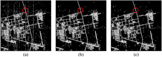
Figure 12.
Comparison of different stripes restore methods. (a) Original image. (b) The neighborhood averaging method. (c) The method based on spectral similarity. (a–c) The red circle emphasizes the effect of different stripes restore methods.
Although the experimental results in Section 3 show that the proposed algorithm has outstanding destriping performance, there are still some possible defects and uncertainties in the design of the algorithm:
- The salt-pepper noise in the GI image is suppressed using the area threshold of the connected component, which may lose some information with respect to artificial lights with areas that are less than the threshold, especially in rural areas where artificial lights are scarce.
- When the impact scale of some road lights is less than the minimum observation capacity of the SDGSAT-1, the width of these roads on the image is often no more than one pixel. In this case, if a stripe appears on this kind of road and the direction of the road is consistent with the stripe, the stripe’s restoration will lose some information (Figure 13). Although this situation is rare, it is still noteworthy.
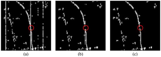 Figure 13. Information loss of different stripes restore methods. (a) Original image. (b) The neighborhood averaging method. (c) The method based on spectral similarity. (a–c) The red circle emphasizes the effect of different stripes restore methods.
- 3.
- The ADSSR algorithm is mainly based on subjective characteristics of images and stripes. Although it is applicable to most images, the subjective characteristics of images and stripes cannot perfectly summarize the actual characteristics in the case of complex weather conditions and poor original image quality, so the performance of the ADSSR algorithm will be degraded. As shown in Figure 14, a cloudy image with invalid relative radiometric correction parameters is selected for testing. Although most of the stripes can be removed, the residual stripe noise is more obvious than that of the cloudless image. Fortunately, the availability of such images is not high.
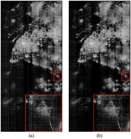 Figure 14. Destriping result of the poor-quality image based on the proposed algorithm. (a) Original image. (b) Destriped image.
Due to the above defects, some image information may be lost when the proposed algorithm is applied. In further research, these problems also need to be solved urgently.
6. Conclusions
In this paper, we proposed a novel destriping algorithm for the GI image. The key idea of the proposed algorithm is to detect and restore stripes based on their characteristics and the spectral similarity of neighboring pixels. Compared with three representative destriping algorithms, the ADSSR algorithm has the best performance from a visual point of view and achieves the lowest RNE and MRD values in all experiments, which indicates that the ADSSR algorithm effectively restores the stripes while preserving the details of the GI image. In addition, the proposed algorithm still maintains outstanding performance and robustness for GI images of different sizes. This provides a feasible method to improve the GI’s image quality.
Author Contributions
D.Z. designed the algorithm and experiments and wrote the manuscript. B.C. (Bo Cheng) supervised the study and reviewed the draft paper. L.S., J.G. and T.L. revised the manuscript and gave some constructive suggestions. B.C. (Bo Chen) and G.W. provided the original data. All authors have read and agreed to the published version of the manuscript.
Funding
This research was funded by the Strategic Priority Research Program of the Chinese Academy of Sciences (Grant Number XDA19010401).
Data Availability Statement
Not applicable.
Acknowledgments
The authors also thank the anonymous reviewers and the editors for their insightful comments and helpful suggestions that improved the manuscript.
Conflicts of Interest
The authors declare no conflict of interest.
References
- Levin, N.; Kyba, C.C.; Zhang, Q.; De Miguel, A.S.; Román, M.O.; Li, X.; Portnov, B.A.; Molthan, A.L.; Jechow, A.; Miller, S.D.; et al. Remote sensing of night lights: A review and an outlook for the future. Remote Sens. Environ. 2020, 237, 111443. [Google Scholar] [CrossRef]
- Grinand, C.; Rakotomalala, F.; Gond, V.; Vaudry, R.; Bernoux, M.; Vieilledent, G. Estimating deforestation in tropical humid and dry forests in Madagascar from 2000 to 2010 using multi-date Landsat satellite images and the random forests classifier. Remote Sens. Environ. 2013, 139, 68–80. [Google Scholar] [CrossRef]
- Masolele, R.N.; Sy, V.N.; Herold, M.; Marcos, D.; Verbesselt, J.; Gieseke, F.; Mullissa, A.G.; Martius, C. Spatial and temporal deep learning methods for deriving land-use following deforestation: A pan-tropical case study using Landsat time series. Remote Sens. Environ. 2021, 264, 112600. [Google Scholar] [CrossRef]
- Smith, V.; Portillo-Quintero, C.; Sanchez-Azofeifa, A.; Hernandez-Stefanoni, J.L. Assessing the accuracy of detected breaks in Landsat time series as predictors of small scale deforestation in tropical dry forests of Mexico and Costa Rica. Remote Sens. Environ. 2019, 221, 707–721. [Google Scholar] [CrossRef]
- Dixit, M.; Chaurasia, K.; Mishra, V.K. Dilated-ResUnet: A novel deep learning architecture for building extraction from medium resolution multi-spectral satellite imagery. Expert Syst. Appl. 2021, 184, 115530. [Google Scholar] [CrossRef]
- Zhang, X.; Cheng, B.; Chen, J.; Liang, C. High-Resolution Boundary Refined Convolutional Neural Network for Automatic Agricultural Greenhouses Extraction from GaoFen-2 Satellite Imageries. Remote Sens. 2021, 13, 4237. [Google Scholar] [CrossRef]
- Yang, Y.; Wu, J.; Wang, Y.; Huang, Q.; He, C. Quantifying spatiotemporal patterns of shrinking cities in urbanizing China: A novel approach based on time-series nighttime light data. Cities 2021, 118, 103346. [Google Scholar] [CrossRef]
- Chen, T.K.; Prishchepov, A.V.; Fensholt, R.; Sabel, C.E. Detecting and monitoring long-term landslides in urbanized areas with nighttime light data and multi-seasonal Landsat imagery across Taiwan from 1998 to 2017. Remote Sens. Environ. 2019, 225, 317–327. [Google Scholar] [CrossRef]
- Zhu, E.; Qi, Q.; Chen, L.; Wu, X. The spatial-temporal patterns and multiple driving mechanisms of carbon emissions in the process of urbanization: A case study in Zhejiang, China. J. Clean. Prod. 2022, 358, 131954. [Google Scholar] [CrossRef]
- Zhang, G.; Guo, X.; Li, D.; Jiang, B. Evaluating the Potential of LJ1-01 Nighttime Light Data for Modeling Socio-Economic Parameters. Sensors 2019, 19, 1465. [Google Scholar] [CrossRef]
- Jiang, W.; He, G.; Liu, H.; Ni, Y. Modelling China economic parameters based on DMSP/OLS nighttime light imagery. Remote Sens. Inf. 2018, 33, 29. [Google Scholar] [CrossRef]
- Elvidge, C.D.; Safran, J.; Tuttle, B.; Sutton, P.; Cinzano, P.; Pettit, D. Potential for global mapping of development via a Nightsat mission. GeoJournal 2007, 69, 45–53. [Google Scholar] [CrossRef]
- Jiang, W.; He, G.; Long, T.; Wang, C.; Ni, Y.; Ma, R. Assessing Light Pollution in China Based on Nighttime Light Imagery. Remote Sens. 2017, 9, 135. [Google Scholar] [CrossRef]
- Jiang, W.; He, G.; Leng, W.; Long, T.; Wang, G.; Liu, H.; Peng, Y.; Yin, R.; Guo, H. Characterizing Light Pollution Trends across Protected Areas in China Using Nighttime Light Remote Sensing Data. ISPRS Int. J. Geo-Inf. 2018, 7, 243. [Google Scholar] [CrossRef]
- Bauer, S.E.; Wagner, S.; Burch, J.B.; Bayakly, R.; Vena, J.E. A case-referent study: Light at night and breast cancer risk in Georgia. Int. J. Health Geogr. 2013, 12, 23. [Google Scholar] [CrossRef]
- Wei, S.; Jiao, W.; Long, T.; Liu, H.; Bi, L.; Jiang, W.; Portnov, B.A.; Liu, M. A Relative Radiation Normalization Method of ISS Nighttime Light Images Based on Pseudo Invariant Features. Remote Sens. 2020, 12, 3349. [Google Scholar] [CrossRef]
- Guo, H.; Chen, H.; Chen, L.; Fu, B. Progress on CASEarth Satellite Development. Chin. J. Space Sci. 2020, 40, 707–717. [Google Scholar] [CrossRef]
- Chen, J.; Cheng, B.; Zhang, X.; Long, T.; Chen, B.; Wang, G.; Zhang, D. A TIR-Visible Automatic Registration and Geometric Correction Method for SDGSAT-1 Thermal Infrared Image Based on Modified RIFT. Remote Sens. 2022, 14, 1393. [Google Scholar] [CrossRef]
- Wang, B.; Bao, J.; Wang, S.; Wang, H.; Sheng, Q. Improved Line Tracing Methods for Removal of Bad Streaks Noise in CCD Line Array Image—A Case Study with GF-1 Images. Sensors 2017, 17, 935. [Google Scholar] [CrossRef]
- Xie, Y.; Wang, J.; Shang, K. An improved approach based on Moment Matching to Destriping for Hyperion data. Procedia Environ. Sci. 2011, 10, 319–324. [Google Scholar] [CrossRef][Green Version]
- Li, M.; Nong, S.; Nie, T.; Han, C.; Huang, L.; Qu, L. A Novel Stripe Noise Removal Model for Infrared Images. Sensors 2022, 22, 2971. [Google Scholar] [CrossRef] [PubMed]
- Han, T.; Goodenough, D.G.; Dyk, A. Detection and Correction of Abnormal Pixels in Hyperion Images. In Proceedings of the IEEE International Geoscience & Remote Sensing Symposium, Toronto, ON, Canada, 24–28 June 2002; Volume 3, pp. 1327–1330. [Google Scholar] [CrossRef]
- Shen, Y.; Liu, X.; Wu, L.; Su, H.; He, H. A Local Spectral-spatial Similarity Measure for Bad Line Correction in Hyperion Hyperspectral Data. Geomat. Inf. Sci. Wuhan Univ. 2017, 42, 99–101. [Google Scholar] [CrossRef]
- Erkan, U.; Gökrem, L.; Enginoğlu, S. Different applied median filter in salt and pepper noise. Comput. Electr. Eng. 2018, 70, 789–798. [Google Scholar] [CrossRef]
- Rasal, T.; Veerakumar, T.; Subudhi, B.N.; Esakkirajan, S. A new approach for reduction of the noise from microscopy images using Fourier decomposition. Biocybern. Biomed. Eng. 2022, 42, 615–629. [Google Scholar] [CrossRef]
- Moradi, M. Wavelet transform approach for denoising and decomposition of satellite-derived ocean color time-series: Selection of optimal mother wavelet. Adv. Space Res. 2022, 69, 2724–2744. [Google Scholar] [CrossRef]
- Wang, C.; Zhang, Y.; Wang, X.; Ji, S. Stripe noise removal of remote image based on wavelet variational method. Acta Geod. Cartogr. Sin. 2019, 48, 1025–1037. [Google Scholar] [CrossRef]
- Pande-Chhetri, R.; Abd-Elrahman, A. De-striping hyperspectral imagery using wavelet transform and adaptive frequency domain filtering. ISPRS J. Photogramm. 2011, 66, 620–636. [Google Scholar] [CrossRef]
- Wang, J.; Huang, T.; Zhao, X.; Huang, J.; Ma, T.; Zheng, Y. Reweighted Block Sparsity Regularization for Remote Sensing Images Destriping. IEEE J. Sel. Top. Appl. Earth Observ. Remote Sens. 2019, 12, 4951–4963. [Google Scholar] [CrossRef]
- Ladjal, S.; Bouali, M. Toward Optimal Destriping of MODIS Data Using a Unidirectional Variational Model. IEEE Trans. Geosci. Remote Sens. 2011, 49, 2924–2935. [Google Scholar] [CrossRef]
- Zhao, S.; Li, J.; Hu, Y.; Liu, X.; Zhang, L. A Fast and Effective Irregular Stripe Removal Method for Moon Mineralogy Mapper (M3). IEEE Trans. Geosci. Remote Sens. 2022, 60, 4600119. [Google Scholar] [CrossRef]
- Chen, Y.; Huang, T.; Zhao, X. Destriping of Multispectral Remote Sensing Image Using Low-Rank Tensor Decomposition. IEEE J. Sel. Top. Appl. Earth Observ. Remote Sens. 2018, 11, 4950–4976. [Google Scholar] [CrossRef]
- Chambolle, A. An algorithm for total variation minimization and applications. J. Math. Imaging Vis. 2004, 20, 89–97. [Google Scholar] [CrossRef]
- Cui, H.; Wu, W.; Zhang, Z.; Han, F.; Liu, Z. Clustering and application of grain temperature statistical parameters based on the DBSCAN algorithm. J. Stored Prod. Res. 2021, 93, 101819. [Google Scholar] [CrossRef]
- Cao, Y.; Yang, M.; Tisse, C. Effective Strip Noise Removal for Low-Textured Infrared Images Based on 1-D Guided Filtering. IEEE Trans. Circuits Syst. Video Technol. 2016, 26, 2176–2188. [Google Scholar] [CrossRef]
- Chang, S.; Yu, B.; Vetterli, M. Adaptive wavelet thresholding for image denoising and compression. IEEE Trans. Image Process. 2000, 9, 2176–2188. [Google Scholar] [CrossRef] [PubMed]
- Donoho, D.; Johnstone, I. Ideal spatial adaptation by wavelet shrinkage. Biometrika 1994, 81, 425–455. [Google Scholar] [CrossRef]


Publisher’s Note: MDPI stays neutral with regard to jurisdictional claims in published maps and institutional affiliations. |
© 2022 by the authors. Licensee MDPI, Basel, Switzerland. This article is an open access article distributed under the terms and conditions of the Creative Commons Attribution (CC BY) license (https://creativecommons.org/licenses/by/4.0/).