DPAFNet: A Multistage Dense-Parallel Attention Fusion Network for Pansharpening

Abstract

Pansharpening is the technology to fuse a low spatial resolution MS image with its associated high spatial full resolution PAN image. However, primary methods have the insufficiency of the feature expression and do not explore both the intrinsic features of the images and correlation between images, which may lead to limited integration of valuable information in the pansharpening results. To this end, we propose a novel multistage Dense-Parallel attention fusion network (DPAFNet). The proposed parallel attention residual dense block (PARDB) module can focus on the intrinsic features of MS images and PAN images while exploring the correlation between the source images. To fuse more complementary information as much as possible, the features extracted from each PARDB are fused at multistage levels, which allows the network to better focus on and exploit different information. Additionally, we propose a new loss, where it calculates the L2-norm between the pansharpening results and PAN images to constrain the spatial structures. Experiments were conducted on simulated and real datasets and the evaluation results verified the superiority of the DPAFNet.

1. Introduction

With the recent launch of many high-resolution (HR) optical satellites, many spatio and temporal informations retrieved by satellites can be used in various research applications such as object detection, ecological protection, and environmental monitoring [1,2,3,4]. Many of these applications require at the highest spatial and spectral resolution to achieve better results. However, due to the limitations of the sensors in terms of physical technology, it is a challenging task to capture both high-resolution spectral and spatial information with a single sensor [5]. Usually, the sensor captures data in two forms: one is HR panchromatic (PAN) image and the other one is low-resolution multispectral (LRMS) image. 1. Pansharpening is to compensate the spatial details of high-resolution panchromatic image (PAN) to low-resolution multispectral image (LRMS), and therefore to obtain multispectral image with high spatial resolution.

In recent years, deep learning-based methods have attracted a lot of attention in computer vision and image processing [6,7], such as image fusion [8], super-resolution [9], image denoising [10], image rain removal, fog removal, and image restoration [11]. In remote sensing images, several researchers employed a convolutional neural network (CNN) to deal with panchromatic image sharpening, where it can effectively extract multi-level automatically. Most existing methods employ supervised learning (SL) to achieve pansharpening since the HRMS can be constrained by Ground Truth (GT), such as PNN [12], BAM [13], and MC-JAFN [14]. Nevertheless, on the one hand, the HRMS will produce artifacts because the GT is synthesized manually. On the other hand, the source images will suffer from spatial destruction due to the decline of the resolution. Such that various unsupervised learning-based (UL) methods are developed to achieve the pansharpening task, such as [15,16,17,18,19], etc. Specifically, these methods can be designed as an encoder–decoder, where the former is to extract multi-level features, whereas the latter is employed to reconstruct the HRMS. Moreover, some attention mechanisms are proposed to further focus on the primary spatial and spectral features in the encoder. However, these methods have some problems as follows:

(1)

Since the low-resolution spectral range of LRMS and the spatial details of PAN images are significantly different, it is difficult to adaptively fuse the spatial details of PAN to all bands of LRMS based on the spectral features. Therefore, it is still a great challenge for the network characterization capability to fully extract spectral and spatial information and fuse them;

(2)

In the encoder, existing networks do not jointly pay attention to spatial structure and spectral information, and single attention can easily cause a mismatch between spatial and spectral information;

(3)

Most networks simply perform single-level decoding in the image reconstruction phase and pay little attention to the loss of information in the extraction phase of features. Such sharpening results in spatial distortion and information distortion easily.

To solve the above problems, we propose a novel pansharpening network, called DPAFNet, where the PAFB module is used for joint spatial and spectral attention. Moreover, a hybrid loss is developed to effectively train our framework. Specifically, the reconstruction loss is to pixel-wisely reconstruct the HRMS image, whereas the spatial loss and the spectral loss are designed from the perspective of the spatial and spectral attention mechanism to further improve the structure of HRMS, respectively. The contributions of this paper are as follows:

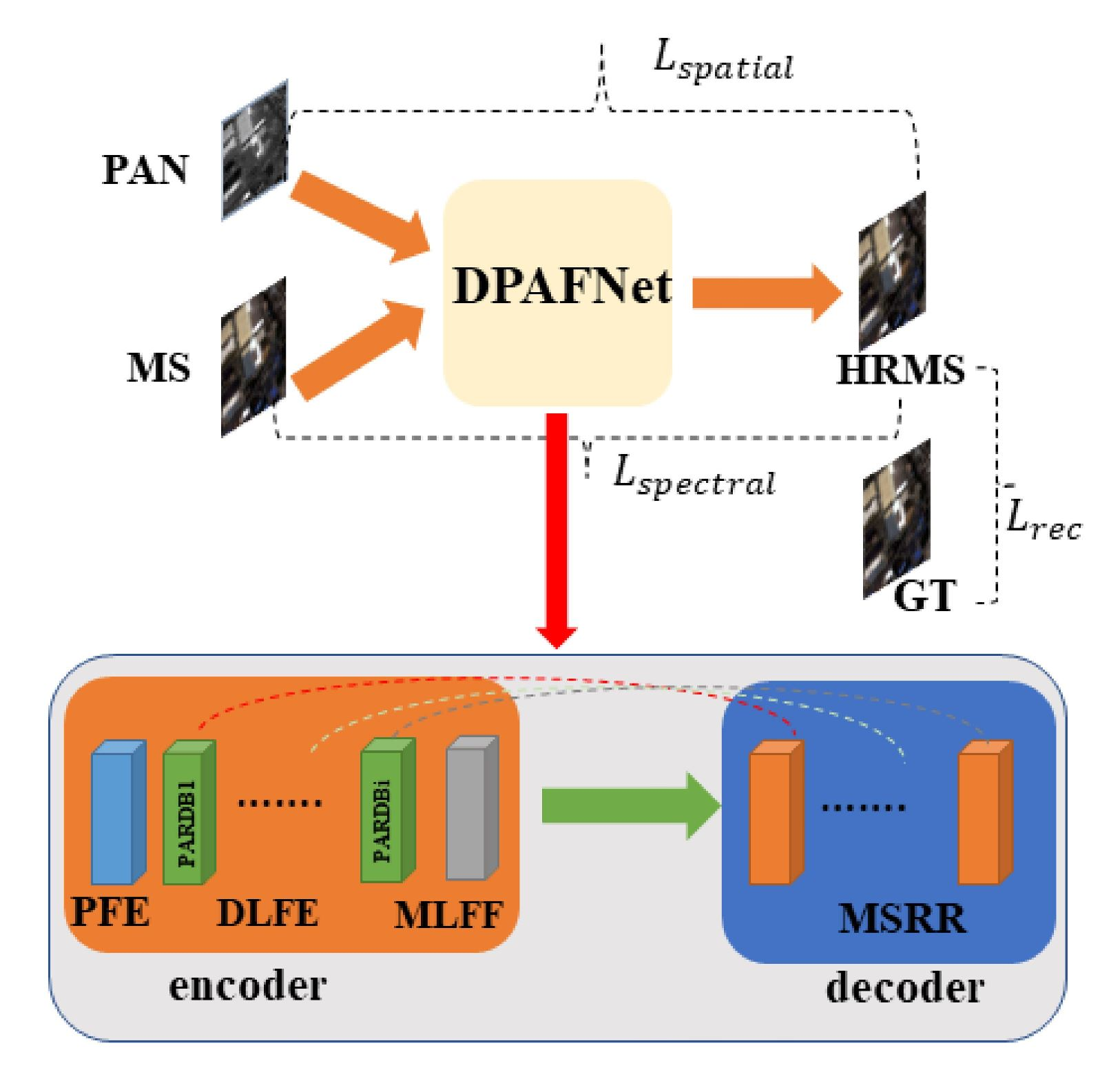
• An end-to-end pansharpening framework. We perform primary and deep feature extraction for PAN and LRMS images. In the deep feature extraction stage, we use parallel attention residual dense block (PARDB) for multi-level extraction, which can extract spatial details and spectral correlations over a wide spectral range. Additionally, PARDB solves the first challenge, which is to promote the representation capability of the network by multi-level feature extraction;
• A parallel attention residual dense block. We propose a parallel attention residual dense block (PARDB) in the encoder, which consists of a Dense Block and a Parallel attention fusion block (PAFB). The PAFB can effectively focus on spectral information and spatial information, and reduce redundancy. Note that the PAFB effectively distinguishes important and redundant information in the feature extraction phase and the fusion phase, solving the second challenge;
• A multi-stage reconstruction network. In the image reconstruction stage, we propose multi-stage reconstruction of residuals (MSRR) for multi-level decoding, meanwhile to supplement the information of image reconstruction. We join the encoded information with the decoded information to act as an information supplement. This effectively solves the third challenge.

2. Related Work

2.1. Traditional Methods

In the past decades, many methods have been proposed for sharpening panchromatic images, which can be divided into three categories: component substitution (CS), multi-resolution analysis (MRA) and super-resolution (SR) paradigm. The main idea of CS methods is to perform a specific transformation of LRMS to separate spatial and spectral information, and then replace the separated spatial information with the spatial information of PAN images. The representative methods based on CS are principal component analysis (PCA) [20], intensity-hue-saturation (IHS) [21], and Gram–Schmidt (GS) [22]. These methods generally have more accurate spatial details, whereas they suffer from significant spectral distortion owing to mismatch the spectral range between PAN and LRMS images.

MRA-based methods, such as high-pass filtering (HPF) [20], smoothing filter-based intensity modulation (SFIM) [23,24], “à trous” wavelet transform (ATWT) [25], decimated Wavelet Transform using an additive injection model (Indusion) [26], and MTF Generalized low-pass (MTF-GLP) [27], employ PAN images to infer the missing spatial details from LRMS images, where they achieve the high frequency features of PAN images through multi-scale decomposition and adaptively inject them into the up-sampled LRMS images. However, the insufficient inference and decomposition algorithms could result spatial distortion, such that they must introduce appropriate strategies.

In the SR methods, PAN and LRMS images are usually considered to be a result of HRMS images’ degradation in spatial structure and spectral information. Therefore, the sharpening of panchromatic images is considered as a recovery problem to recover the HRMS from the degraded image. According to the SR methods, the PAN and LRMS images can be considered as a linear combination and blurred versions of HRMS images, respectively. Hence, these methods, including sparse representation [28], variational [29], model-based fusion using PCA and wavelets(FE-HPM) [30], model-based fusion using PCA and wavelets (PWMBF) [31], etc., recover images mainly by constructing constraint terms. Nevertheless, the sparse representation often results in spatial distortion since the destruction of the spatial structure appear spatial distortion.

2.2. Deep-Learning Based Methods

2.2.1. Network Backbone for Pansharpening

Resorting to CNN and Generative Adversarial Network (GAN), many deep learning-based methods are introduced to achieve the pansharpening task. For some SL-based algorithms, Masi et al. [12] proposed PNN by interpolating the LRMS image with the PAN image. Jin et al. [13] proposed a simple and effective bilateral activation mechanism (BAM) to avoid simply performing a negative truncation. However, the HRMS images will suffer from unreasonable artifacts in the training phase. Additionally, how to avoid the information loss of the LRMS during the downsampling operation is always an open problem.

To alleviate the defects in SL-based schemes, UL-based methods are developed to directly reconstruct the HRMS image without Wald Protocol [32] in the encoder. Representatively, ref. [15] proposed an iterative network and a guided strategy to further extract features from the source images. Ref. [16] employed registration learning in pansharpening (UPSNet) to avoid dedicated registering the source images. Ref. [18] pre-trained their framework by SL, whereas the whole architecture is fine-tuned by UL. The other two methods, refs. [17,19], generate the HRMS images by a unified CNN-based backbone and GAN network, respectively. Nevertheless, the reconstructional results will cause spectral distortion and spatial degradation due to the uncertainty of UL. Moreover, the loss function in these methods does not further refine the constraint spatial structure and spectral information, resulting in distortion of the fused results.

2.2.2. Attention Mechanism for Pansharpening

A good attention mechanism is a core factor to extract spectral and spatial features, such that it is widely introduced in pansharpening. Specifically, Zhang et al. [33] designed a bidirectional pyramid network (BDPN) to ensure the network gives more attention to local information. Lei et al. [34] proposed a multi-branching-based attention network to adequately extract spatial and spectral information. Guan et al. [35] employed a dual-attention-based network with a three-stream structure to fully combine the correlation and relevance of the source images. Differently, ref. [36] first obtain the spatial features of the source images by a high-pass filter, then a dual-branch attentional fusion network is proposed to enhance the spectral resolution of the HRMS image. Recently, the vision transformer (ViT) [37] has been widely used in computer vision tasks because the self-attention mechanism can focus on the global features of the source images. Based on this, Meng et al. [38] designed a self-attention-based encoder to extract both local and global information and finally reconstruct the results by stitching and upsampling operations. Although the attention networks in their methods perform effectively, they still suffer from spatial and spectral distortion since the attention mechanisms are not constrained by the loss function.

Compared with other methods, our DPAFNet, in its en-coder, proposes a multistage Dense-Parallel attention net-work to adequately extract spatial and spectral features. Moreover, we develop a hybrid attention loss according to the parallel attention mechanism to effectively train our framework.

3. Methodology

3.1. Problem Statement

The PAN images have rich spatial information, whereas rich spectral information is exhibited by LRMS images. The work in this paper is to fuse of PAN and LRMS rich important to generate HRMS. In order to accomplish this task, we propose a new method that adaptively fuses spectral and spatial information in multiple stages. Let $M\in {\mathbb{R}}^{h\times w\times B}$ represents LRMS image, B is the number of bands. Moreover, $h\times w$ denotes the spatial size of each band number. $P\in {\mathbb{R}}^{H\times W}$ present the PAN image in a single band, generally $H=r\times h$, $W=r\times w$, where r represents the ratio of the spatial resolution of the LRMS and PAN images. Most traditional approaches follow the following convergence framework [39]:

$$X=\widehat{M}+R=\widehat{M}+\phi (\widehat{M},P),$$

(1)

where $X\in {\mathbb{R}}^{H\times W\times B}$ is the pansharpened HRMS image. Additionally, $\widehat{M}\in {\mathbb{R}}^{H\times W\times B}$ is the upsampled version of LRMS [27], which constitutes a high-resolution multispectral image. $R\in {\mathbb{R}}^{H\times W\times B}$ can be considered as the residual, and the detail information of LRMS and PAN images are extracted by the function $\phi$ to compose HRMS. Therefore, we can rely on Equation (1) to design our network.

3.2. Network Framework

Our proposed network is shown in Figure 1. In the data preparation phase, we first up-sample the LRMS to the same size as P. Then the up-sampled image LRMS (marked as $\widehat{M}\in {\mathbb{R}}^{H\times W\times B}$ with P in the spectral dimension is concatenated as the input $I\in {\mathbb{R}}^{H\times W\times (B+1)}$ to the DPAFNet. In Figure 1, DPAFNet consists of four main components: primary feature extraction (PFE), Deep-level feature extraction (DLFE), multi-level feature fusion (MLFF), multi-stage reconstruction of residuals (MSRR). First, we use PFE module for primary feature extraction, which consists of a basic stack of convolutional layers and activation functions:

$$F_S=H_{PFE}\left(I\right)$$

(2)

where $H_{PFE}(·)$ denotes the PFE module, then the feature $F_S$ is fed into the DLFE module. DLFE module consists of a stack of i PARDBs. The output $F_i$ passing through i-th PARDBs can be calculated by:

$$\begin{array}{cc}\hfill F_i& =H_{PARDB,i}\left(F_{i-1}\right)\hfill \\ \hfill & =H_{PARDB,i}(\dots \left(H_{PARDB,1}\left(F_S\right)\right)\dots ),\hfill \end{array}$$

(3)

where $H_{PARDB}(·)$ denotes the i-th PARDB block. The output of each PARDB is fed into the MLFF module, which is represented as follows:

$$F_{MLF}=H_{MLFF}(F_1,\dots ,F_i),$$

(4)

where $H_{MLFF}(·)$ represents MLFF module, $F_{MLF}$ is multi-level feature fusion. Finally, we feed $F_{MLF}$ into the MSRR module, which is calculated as follows:

$$R_i=H_{MSRR}\left(F_{MLF}\right),$$

(5)

where $R_i$ is the output of the MSRR module.

3.3. DLFE

We design a new module PARDB to extract deep features, the spectral attention module and spatial attention module modules are first introduced, and then the composition of the PAFB module is described. Finally, it introduces how to embed PAFB into Dense block to form PARDB module.

3.3.1. Spectral Attention Module

The primary features extracted by PFE contain different cross-channel information and contribute differently to the fusion process. Therefore, more focuses on the spectral information feature maps that are highly correlated with the input information, and redundant information other than that should be suppressed.

The module structure of spectral attention is shown in Figure 2, To focus more on the spectral information, we use a bottleneck strategy to suppress redundant information, for which we set the size of the convolution kernel to $1\times 1\times C\times (C/r)$ and $1\times 1\times (C/r)\times C$. Then, gradually aggregate the spectral information through a convolution block. Finally, the features are compressed into a vector ($M_{spe}$) by averaging pooling, and then each value of the vector is compressed to [0, 1] by the sigmoid function. The size of the attention vector is the same as the $U_{ori}$ channel. The output of the spectral attention module is as follows:

$$U_{spe}=U_{ori}\otimes M_{spe},$$

(6)

where $U_{ori}$ represents the input of the spectral attention module, ⊗ is the multiplication, $U_{spe}$ depicts the output of the spectral attention module.

With the spectral attention module, the network can better suppress redundant information, improve the correlation between channels, and reduce the spectral distortion of the fusion process.

3.3.2. Spatial Attention Module

Unlike the spectral attention module that compresses spatial information into a single channel, spatial attention module aims to highlight the most spatially informative regions of the input, while each feature map contains different spatial information. Usually the high-frequency information in textured areas is difficult to sharpen, while the low-frequency information in smooth areas is ignored. Therefore, we take advantage of the spatial relationships by adding a spatial attention module.

For the spatial attention module as shown in Figure 2, it is composed of a convolutional layer, two bottleneck blocks and two following convolutional layers. The bottleneck blocks are similar to residual structures, mainly to reduce the number of parameters and to suppress redundant information. Finally, each value of the feature vector ($M_{spa}$) is compressed to [0, 1] by sigmoid. The output of the spatial attention module is as follows:

$$U_{spa}=U_{ori}\otimes M_{spa},$$

(7)

where $U_{ori}$ represents the input of the spatial attention module, ⊗ is the multiplication, $U_{spa}$ is the output of the spatial attention module.

By improving the location information related to sharpening with the spatial attention module, the feature representation of our network is improved.

3.3.3. PAFB

To better fuse the spectral and spatial information, we connect the spectral attention and spatial attention modules in parallel, while concatenating the results of both with the input. Finally, the stacked features are further encoded by two convolutional layers. The output of the PAFB module is as follows:

$$U_{PA}=f_2(\delta ·\left(f_1\left(\left[[U_{spe},U_{spa},U_{ori}]\right]\right)\right)+b_1)+b_2$$

(8)

where $\left[\right[·\left]\right]$ denotes the concatenation operation, $f_i$ denotes the convolutional layer with a kernel size of $3\times 3$, $\delta (·)$ represents the activation function ReLU. Additionally, $b_1$ and $b_2$ are the bias of the convolutional layers, respectively.

3.3.4. PARDB

We embed the PAFB into the dense block, so that the PARDB has a better fusion effect, as shown in Figure 3.

Let $F_{i-1}$ be the input of the i-th PARDBs. Firstly, the local features are extracted by several dense layers and ReLU. Then the different local features are fused and downscaled to form the local feature $U_{ori}$. We add PAFB after generating the local features and adaptively let the refinement of the local features fuse (the result is as $U_{PA}$). Finally, a skip connection is used to add $U_{PA}$ and $F_{i-1}$ to achieve a feature complementary function. This connection can effectively fuse low-level features with high-level features. The output $F_i$ of the i-th PARDBs is as follows:

$$F_i=U_{PA}\oplus F_{i-1},$$

(9)

where ⊕ denotes the elementwise sum operation. PARDB combines the advantages of both dense block and PAFB, which can fully extract the features of different layers and effectively fuse the spectral and spatial information.

3.4. MLFF Module

To obtain useful spectral and spatial information, we use MLFF to adaptively combine multi-level features. The output of the MLFF module is as follows:

$$\begin{array}{cc}\hfill F_{MLF}& =H_{MLFF}(F_1,\dots ,F_i)\hfill \\ \hfill & =H_{PAFB}\left(f_1\left(\left[[F_1,\dots ,F_i]\right]\right)+b1\right),\hfill \end{array}$$

(10)

where $\left[\right[·\left]\right]$ denotes the concatenation operation, $f_1$ depicts the convolutional layer with a kernel size of $3\times 3$ for global feature fusion, whereas $b_1$ represents the bias of the convolutional layer. Moreover, to better suppress redundant information, we add PAFB in MLFF, where it enables the fusion of multi-level features, and suppresses redundant information.

3.5. MSRR Module

In the image reconstruction part, in order to obtain a better reconstructed image. We superimpose multiple $R{R}_i$ blocks while using skip connections to sum the outputs of different PARDB blocks with them, and the final output is the reconstructed residuals. The output of the MSRR module is as follows:

$$\begin{array}{cc}\hfill R_i& =H_{R{R}_i}(R_{i-1}+F_i)\hfill \\ \hfill & =H_{R{R}_i}(\dots \left(H_{R{R}_1}(F_{MLF}+F_1)\right)\dots ),\hfill \end{array}$$

(11)

where $H_{R{R}_i}(·)$ denotes the $R{R}_i$ block, which is stacked by two convolution and ReLU functions.

3.6. Loss Function

Note that the loss function is an important factor in training deep networks. In this paper, we propose hybrid loss to optimize our network.

3.6.1. Reconstruction Loss

Most previous sharpening methods utilize the $L_2$-norm as the loss function for parameter optimization of the network, such as [40], etc. However, the $L_2$-norm suffers from ambiguity and over-sharpening, such that $L_1$-norm have been generally employed in pansharpening [35,36]. Inspired by these methods, we use $L_1$ as the reconstruction loss, as follows:

$$L_{rec}=\frac{1}{N}\sum _{i=1}^N\left|\right|G{T}_i-X_i{\left|\right|}_1,$$

(12)

where $G{T}_i$ denotes the i-th Reference image, and $X_i$ represents the i-th image predicted by the network. N denotes the number of trained pairs of images.

3.6.2. Spatial Loss

To preserve spatial structure in pansharpening, we transform the sharpening result into a single band by applying a band transformation. Then, we use $L_2$ parametric constraints to constrain the difference between the single band result and the PAN image at the pixel level. our spatial structural loss is defined as:

$$L_{spatial}=\frac{1}{N}\sum _{i=1}^N\left|\right|P_i-{\widehat{X}}_i{\left|\right|}_2,$$

(13)

where $P_i$ denotes the i-th source PAN image, ${\widehat{X}}_i$ represents each band of the i-th multispectral image predicted by the network and N denotes the number of trained pairs of images.

3.6.3. Spectral Loss

SAM is employed to quantify the spectral distortion, here, we use the spectral vector at each position as a spectral feature. Then, SAM loss [41] is introduced to constrain the spectral distortions, which can be defined as:

$$L_{spectral}=\frac{SAM(X_i,G{T}_i)}{\pi }$$

(14)

$$SAM(X_i,G{T}_i)=\frac{1}{MN}\sum _{i=1}^{MN}arccos\left(\frac{〈X_i,G{T}_i〉}{\left|\right|X_i{\left|\right|}_2\left|\right|G{T}_i{\left|\right|}_2}\right),$$

(15)

where $X_i$ and $G{T}_i$ are the i-th spectral vectors of two images, $〈·〉$ is the inner product, $\left|\right|·{\left|\right|}_2$ denotes the $L_2$-norm of a vector, and $SAM(X_i,G{T}_i)$ is the average of SAM values overall pixel location. The loss function we used for training is as follows:

$$L=\alpha L_{rec}+\beta L_{spatial}+\gamma L_{spectral},$$

(16)

where L represents the total loss function, $L_{rec}$ denotes the reconstruction loss, $L_{spatial}$ denotes the spatial loss, $L_{spectral}$ denotes the spectral loss, $\alpha$, $\beta$, $\gamma$ are regularization constants. In this paper, we set $\alpha =1.0$, $\beta =0.07$, $\gamma =0.03$.

4. Experiments

4.1. Datasets and Setup

In our experiments, the two real datasets are from IKONOS and WorldView-2 (WV-2) sensors. The details are shown in

Table 1. Details of the Two Sensors Used in Our Experiments.

Sensor	Band	MS	PAN	Radiometric	Scaling
IKONOS	4	4 m	1 m	11 bits	4
WV-2	8	2 m	0.5 m	11 bits	4

. Based on the number of bands of different satellites, we trained the networks supporting 4-band and 8-band respectively. The dataset of IKONOS includes 200 PAN and LRMS pairs with the spatial size of 1024 × 1024 and 256 × 256, meanwhile, the dataset of WV-2 contains 500 PAN/LRMS pairs with the spatial size of 1024 × 1024 and 256 × 256. Due to a lack of ground truth, we followed Wald’s protocol [32] to generate the simulated dataset, the spatial resolution of the simulated dataset is 1/4 of the real dataset. Note that, in the training phase, the Wald’s protocol is always conducted to the dataset to ensure resolution reduction. Meanwhile, original LRMS are used as ground truth (GT) for training the network. For each simulated dataset, we selected 80% and 20% of the dataset for training and testing, respectively.

Our model is trained using the Pytorch package on a computer with Nvidia GeForce RTX 2080 GPUs. We use Adamw to learn to minimize loss, with the related parameters ${\beta }_1=0.5$, ${\beta }_2=0.999$, and $ϵ=1\times {10}^{-8}$. Moreover, all the convolutional layers are with bias and the learning rate is set to $1\times {10}^{-5}$, whereas the relevant parameters are set to $\beta =0.07$, $\gamma =0.03$, respectively.

4.2. Compared Methods

To better verify the advanced nature of DPAFNet, we selected eight representative algorithms, including PCA [20], IHS [21], GS [22] from CS, HPF [20], SFIM [23]. Ref. [24], Induison [26] from MRA, FE-HPM [30], PWMBF [31] from SR and six deep learning-based approaches, such as PNN [12], DRPNN [17], PercepPan [18], PGMAN [19], BAM [13], and MC-JAFN [14]. We reimplemented the BAM, MC-JAFN, DRPNN, PercepPan and PGMAN by Pytorch, and the rest of the methods were based on the MATLAB platform [39]. In addition, MS image interpolation was included, using a polynomial kernel with 23 coefficients [27], which is called EXP. To achieve a better performance, all parameters were set according to the original paper.

4.3. Evaluation Metrics

In the process of pansharpening, the lack of reference images limits the results of image evaluation. To solve this challenge, two comparison methods are proposed. The first one is to downsample MS and PAN images to reduce the resolution based on Wald’s protocol [32] and use the original MS image as the reference image. Another one is to perform quality evaluation directly on the real dataset without the reference image. Due to the presence of reference images, some metrics were proposed to evaluate the quality of sharpening of reduced resolution images. To evaluate our pansharpening results more comprehensively, we chose spectral angle mapper (SAM) [42] and Q4 [43] or Q8 [44] to measure the spectral distortion, spatial correlation coefficient (SCC) [45] to measure the spatial distortion. Universal image quality index averaged over the bands(Q) [46] and Erreur Relative Globale Adimensionnelle de Synthèse (ERGAS) [47] are used for global indexing. Note that Q4, Q8, Q, and SCC are from 0 to 1, and the larger of these metrics indicate a better HRMS image. SAM and ERGAS are from 0 to any positive number, whereas the smaller they are, the better the fused result. When evaluating metrics at their original resolution, using the quality without reference (QNR) [48] index, at the same time it contains two components $D_{\lambda }$ and $D_s$, which the quality the spectral and spatial distortion, respectively. Similarly, all of these three metrics range from 0 to 1, in which lower references of $D_{\lambda }$, $D_s$, and higher references of QNR denote a preferable fused image.

4.4. Visual and Quantitative Assessments

We show the image sharpening visual results and quantitative analysis between DPAFNet and other state-of-the-art 15 methods at reduced-resolution and full-resolution.

Reduced Resolution Analysis: We started the analysis at a reduced resolution when the original MS was considered the ground truth (GT). The spatial resolution of the input MS/PAN image is reduced to 1/4 of the original image. The detailed index evaluation results are shown in

Table 2. Quantitative Evaluation for Reduced IKONOS Dataset. The Best Results are Shown in Bold.

	Q4	Q	SAM	ERGAS	SCC
Reference	1	1	0	0	1
EXP	0.6103	0.6121	3.4047	3.3219	0.6670
PCA	0.7604	0.7419	3.6551	2.6815	0.8711
IHS	0.7286	0.7425	3.4511	2.5583	0.8828
GS	0.7688	0.7765	3.2024	2.4349	0.9055
PRACS	0.8109	0.8088	2.9041	2.1432	0.9057
HPF	0.8237	0.8238	2.9118	2.0690	0.9110
SFIM	0.8274	0.8275	2.8673	2.0303	0.9152
Indusion	0.7676	0.7748	3.1378	2.5851	0.8718
FE-HPM	0.8471	0.8464	2.7843	1.8539	0.9248
PWMBF	0.7934	0.7884	3.1957	2.1778	0.9108
PNN	0.8741	0.8781	2.2769	1.5588	0.9453
DRPNN	0.9179	0.9210	1.5225	2.1977	0.9518
PercepPan	0.8994	0.9036	1.6896	2.4813	0.9416
PGMAN	0.9046	0.9073	1.6433	2.3442	0.9450
BAM	0.9040	0.9058	2.3844	1.6073	0.9439
MC-JAFN	0.9215	0.9230	2.1657	1.4942	0.9527
Ours	0.9320	0.9331	1.9569	1.3916	0.9595

and

Table 3. Quantitative Evaluation for Reduced WorldView-2 Dataset. The Best Results are Shown in Bold.

	Q8	Q	SAM	ERGAS	SCC
Reference	1	1	0	0	1
EXP	0.6074	0.6113	7.9286	8.7566	0.5099
PCA	0.8228	0.8226	7.4781	6.1551	0.9127
IHS	0.8251	0.8195	8.0139	6.2805	0.8944
GS	0.8223	0.8224	7.4535	6.1614	0.9136
HPF	0.8631	0.8617	7.0718	5.5755	0.9069
SFIM	0.8651	0.8637	7.1246	5.5025	0.9097
Indusion	0.8214	0.8214	7.3738	6.4526	0.8600
FE-HPM	0.8929	0.8906	6.9836	5.0537	0.9098
PWMBF	0.8963	0.8894	7.3735	5.0706	0.9176
PNN	0.9251	0.9256	5.8696	4.2395	0.9372
DRPNN	0.9566	0.9583	3.3716	5.2837	0.9610
PercepPan	0.9575	0.9586	3.3543	5.1202	0.9606
PGMAN	0.9603	0.9614	3.2299	4.9735	0.9638
BAM	0.9599	0.9605	5.0647	3.2334	0.9630
MC-JAFN	0.9629	0.9636	4.8988	3.1057	0.9664
Ours	0.9662	0.9670	4.6440	2.9638	0.9699

.

From Table 2 and Table 3, it can be seen that the deep learning approach has significantly improved over the traditional approach in terms of quantitative metrics. Among the five DL methods mentioned in this paper, our method has the best performance, especially in the WV-2 dataset.

The results of the IKONOS and WV-2 dataset visualizations are shown in Figure 4 and Figure 5, respectively. In the first row, we show the GT image and the results of different methods of sharpening. Since there is a reference image, to better compare the detail loss, in the second row we show the error images corresponding to each method. From Figure 4 and Figure 5, it can be seen that the sharpening results of traditional methods always have severe spectral distortion and their color saturation is lower than that of the reference image. Additionally, the spatial resolution of the sharpening results produced by conventional methods is severely distorted, especially in PCA [20] and IHS [21], which can be seen more clearly in the error images. By contrast, we can see that all the deep learning methods can better preserve the spectral information and spatial structure, meanwhile, producing sharpening results with rich edge information and saturated colors. According to the error image, our sharpening result is closer to the reference image, which proves that our method can well preserve spectral information and spatial structure.

Full Resolution Analysis: In the reduced resolution experiments, we proved to be methodologically optimal by qualitative and quantitative analysis. However, in real applications, GT is not available and both MS and PAN images are at the resolution of satellite capture. To evaluate the performance at full resolution, we show the quantitative analysis of IKONOS and WV-2 dataset in

Table 4. Quantitative Evaluation for Real Dataset. The Best Results are Shown in Bold.

Dataset	IKONOS			WorldView-2
Metric	${\mathit{D}}_{\mathit{\lambda }}$	${\mathit{D}}_{\mathit{s}}$	QNR	${\mathit{D}}_{\mathit{\lambda }}$	${\mathit{D}}_{\mathit{s}}$	QNR
Reference	0	0	1	0	0	1
EXP	0.0000	0.0973	0.9027	0.0000	0.0630	0.9370
PCA	0.0785	0.1775	0.7666	0.0196	0.1057	0.8768
IHS	0.1294	0.2311	0.6808	0.0231	0.1005	0.8787
GS	0.0802	0.1879	0.7537	0.0193	0.1040	0.8787
HPF	0.1224	0.1832	0.7245	0.0475	0.0882	0.8686
SFIM	0.1212	0.1798	0.7285	0.0444	0.0856	0.8738
Indusion	0.1069	0.1504	0.7663	0.0335	0.0795	0.8897
FE-HPM	0.1386	0.1935	0.7035	0.0607	0.1079	0.8381
PWMBF	0.1628	0.2236	0.6575	0.0958	0.1461	0.7724
PNN	0.0737	0.1064	0.8395	0.0564	0.0728	0.8749
DRPNN	0.0499	0.0984	0.8608	0.0394	0.0882	0.8758
PercepPan	0.0366	0.0961	0.8742	0.0324	0.0955	0.8752
PGMAN	0.0388	0.1049	0.8648	0.0228	0.0934	0.8860
BAM	0.0348	0.0820	0.8865	0.0251	0.0939	0.8833
MC-JAFN	0.0294	0.0741	0.8987	0.0390	0.0748	0.8891
Ours	0.0299	0.0713	0.9009	0.0253	0.0759	0.9007

. In full-resolution evaluation, deep learning methods always give better results, especially in the IKONOS dataset. In addition to that, deep learning methods also obtain better results when in the WV-2 dataset, but not always better than traditional methods, such as Indusion [26]. Although our proposed method does not obtain the optimal $D_{\lambda }$ and $D_s$, we obtain the best QNR on two different datasets. Figure 6 and Figure 7 show the visualization results of different methods of sharpening at full resolution. For the IKONOS dataset shown in Figure 6, pansharpened images of PCA, IHS, GS, HPF, Indusion, FE-HPM, PWMBF loss some image details. In particular, GS not only loses some information but also produces severe spectral distortions. By contrast, the resulting images of the five deep learning methods are given without severe spectral distortions.

Additionally, to better compare the priority of each method, we enlarged the sharpened image of each method (marked by the red box ) and displayed it in the appropriate position. From the enlarged area of EXP in Figure 6, we can see that our network could recover some color features, indicating that the network has good spectral preservation ability. From the zoomed-in region in Figure 7, it can be seen that the conventional methods cannot fully recover the details of PAN images, and the sharpening result of PNN, DRPNN, PercepPan, PGMAN, BAM and MC-JAFN looks unnatural. In contrast, our proposed network preserves more details and looks more natural. By visual and quantitative comparison at full resolution, our proposed network outperforms both traditional and state-of-the-art deep learning methods in terms of spectral preservation.

4.5. Parameter Analysis

The proper loss function is very important for the training of neural networks. To achieve good sharpening results, we analyzed the two parameters $\beta$ and $\gamma$ of the loss function in

Table 5. Average Quantitative Metrics of Different Regularization Parameters in $\beta L_{spatial}$ and $\gamma L_{spectral}$. The Best Results are Shown in Bold.

Parameter		Metrics
$\mathbf{\beta }$	$\mathbf{\gamma }$	Q4	Q	SAM	ERGAS	SCC
	0.01	0.9312	0.9322	1.9747	1.4045	0.9589
0.05	0.03	0.9320	0.9333	1.9576	1.3917	0.9595
	0.05	0.9326	0.9336	1.9619	1.3993	0.9595
	0.01	0.9307	0.9317	1.9779	1.4034	0.9587
0.07	0.03	0.9320	0.9331	1.9569	1.3916	0.9595
	0.05	0.9319	0.9329	1.9613	1.3996	0.9593
	0.01	0.9320	0.9330	1.9562	1.3934	0.9594
0.09	0.03	0.9313	0.9324	1.9685	1.4016	0.9592
	0.05	0.9319	0.9330	1.9544	1.3957	0.9593

. Hence, we set $\beta$ to 0.05, 0.07, and 0.09, respectively. Tthe other parameter was set to 0.01, 0.03, and 0.05 to achieve good fusion results. We used different parameters to quantify the analysis. Table 5 shows the results of quantitative indexes with different parameters. The SAM, ERGAS, SCC can achieve the best results when $\beta =0.07$ and $\gamma =0.03$. To summarize, we chose $\beta =0.07$ and $\gamma =0.03$ to achieve the best sharpening results.

4.6. Ablation Study

To verify the impact of different modules on our network, we conducted ablation experiments of network and loss. They are shown in

Table 6. Comparison of Fusion Performance on IKONOS Dataset Between Our Method and Its Degraded Versions. The Best Results are Shown in Bold.

	Ablation				Metrics
Skip	SpectralA	SpatialA	Q4	Q	SAM	ERGAS	SCC
✗	✗	✗	0.9263	0.9269	2.0581	1.4541	0.9553
✗	✓	✓	0.9280	0.9289	2.0361	1.4402	0.9563
✓	✗	✗	0.9283	0.9290	2.0231	1.4339	0.9569
✓	✗	✓	0.9307	0.9317	1.9709	1.4100	0.9586
✓	✓	✗	0.9309	0.9323	2.0277	1.4383	0.9568
✓	✓	✓	0.9320	0.9331	1.9569	1.3916	0.9595
${\mathit{L}}_{\mathit{rec}}$	${\mathit{L}}_{\mathit{spatial}}$	${\mathit{L}}_{\mathit{spectral}}$	Q4	Q	SAM	ERGAS	SCC
✓	✗	✗	0.9313	0.9323	1.9838	1.4069	0.9589
✓	✓	✗	0.9319	0.9331	1.9580	1.3942	0.9594
✓	✗	✓	0.9315	0.9330	1.9572	1.3927	0.9594
✓	✓	✓	0.9320	0.9331	1.9569	1.3916	0.9595

.

4.6.1. Ablation to Network

To verify the usefulness of the different modules, we divided the network ablation into five parts. The first one is the network with “no skip connections and no attention”, i.e., no feature compensation in reconstructed images no dual-attention mechanism. The second one is the net-work with “no skip connection”, whereas the third one denotes the network with only “skip connection”, i.e., the PAFB module was removed in the encoder. As shown in Table 6, the quantitative results show that the skip connection and parallel attention block provide contributions to our pansharpening network. Moreover, we also perform the single attention block in the encoder, such that the network turns to only spatial and spectral attention mechanism, respectively. We can see that each metric is inferior to the parallel-attention network, whereas they are all superior to no PAFB module. That is to say, each attention part and the skip connection is a core factor to generate a better HRMS image.

4.6.2. Ablation to Loss Function

We performed three ablations of the loss function to validate its availability, with only reconstruction loss ($L_{rec}$), no spectral loss ($L_{rec}+L_{spatial}$), and no spatial loss ($L_{rec}+L_{spectral}$). As illustrated in Table 6, our method produces the best results on each metric, especially SAM and ERGAS improve by 2.69% and 1.53%, respectively. These results indicate that the $L_{spatial}$ and $L_{spectral}$ further constrain the fidelity of spatial and spectral information on the basis of reconstruction loss, and improve the fidelity of spatial and spectral information.

4.7. Discussion of Spatial Loss

In this sub-section, we are dedicated to discussing the effectiveness of spatial loss. Specifically, we turn the spatial loss ($L_{spatial}$) into the structural similarity loss ($L_{ssim}$) [49].

Table 7. The quantitative comparison between the spatial loss and structure similarity loss. The Best Results are Shown in Bold.

Spatial Loss	Q4	Q	SAM	ERGAS	SCC
$L_{rec}+L_{spatial}+L_{spectral}$	0.9320	0.9331	1.9569	1.3916	0.9595
$L_{rec}+L_{ssim}+L_{spectral}$	0.9342	0.9357	1.9791	1.4089	0.9588

illustrates the quantitative evaluation of these two losses, in which $L_{spatial}$ performs better than $L_{ssim}$ in terms of SAM, ERGAS, and SCC, while the $L_{ssim}$ provides better results for Q4 and Q than $L_{spatial}$. However, it is noted that the difference between the two losses in Q4 and Q is not obvious, because these two metrics only focus on a single band. Although the $L_{ssim}$ can enhance the spatial structure to some extent, it suffers from mismatching with the corresponding bands, such that the overall spectral trend is significantly descending, i.e., ERGAS and SAM. These quantitative results imply that the proposed spatial loss can further improve fusion quality.

5. Conclusions

In this paper, we proposed a novel panchromatic image sharpening framework, called DPAFNet. By utilizing PARDB, our network can simultaneously learn the unique information of the image and the correlation between MS and PAN images. Instead of single-scale pansharpening, we performed the PAFB module for multi-level feature fusion in the training phase. Furthermore, a novel spatial loss was introduced; the results were able to preserve more spatial structure features from the PAN images. Experiments were carried out on simulated data sets and real datasets, where the visual and quantitative results verified the advantages of our DPAFNet.

References

1. Wang, J.; Gong, Z.; Liu, X.; Guo, H.; Lu, J.; Yu, D.; Lin, Y. Multi-Feature Information Complementary Detector: A High-Precision Object Detection Model for Remote Sensing Images. Remote Sens. 2022, 14, 4519. [Google Scholar] [CrossRef]
2. Zheng, C.; Abd-Elrahman, A.; Whitaker, V.; Dalid, C. Prediction of Strawberry Dry Biomass from UAV Multispectral Imagery Using Multiple Machine Learning Methods. Remote Sens. 2022, 14, 4511. [Google Scholar] [CrossRef]
3. Shalaby, A.; Tateishi, R. Remote sensing and GIS for mapping and monitoring land cover and land-use changes in the Northwestern coastal zone of Egypt. Appl. Geogr. 2007, 27, 28–41. [Google Scholar] [CrossRef]
4. Weng, Q. Thermal infrared remote sensing for urban climate and environmental studies: Methods, applications, and trends. ISPRS J. Photogramm. Remote Sens. 2009, 64, 335–344. [Google Scholar] [CrossRef]
5. Zhang, Y. Understanding image fusion. Photogramm. Eng. Remote Sens 2004, 70, 657–661. [Google Scholar]
6. Ren, Z.; So, H.K.H.; Lam, E.Y. Fringe pattern improvement and super-resolution using deep learning in digital holography. IEEE Trans. Ind. Inform. 2019, 15, 6179–6186. [Google Scholar] [CrossRef]
7. Meng, N.; Zeng, T.; Lam, E.Y. Spatial and angular reconstruction of light field based on deep generative networks. In Proceedings of the 2019 IEEE International Conference on Image Processing (ICIP), Taipei, Taiwan, 22–25 September 2019; IEEE: Piscataway, NJ, USA, 2019; pp. 4659–4663. [Google Scholar]
8. Zhang, G.; Nie, R.; Cao, J. SSL-WAEIE: Self-Supervised Learning with Weighted Auto-Encoding and Information Exchange for Infrared and Visible Image Fusion. IEEE/CAA J. Autom. Sin. 2022, 9, 1694–1697. [Google Scholar] [CrossRef]
9. Dong, C.; Loy, C.C.; He, K.; Tang, X. Image super-resolution using deep convolutional networks. IEEE Trans. Pattern Anal. Mach. Intell. 2015, 38, 295–307. [Google Scholar] [CrossRef] [Green Version]
10. Dou, H.X.; Pan, X.M.; Wang, C.; Shen, H.Z.; Deng, L.J. Spatial and Spectral-Channel Attention Network for Denoising on Hyperspectral Remote Sensing Image. Remote Sens. 2022, 14, 3338. [Google Scholar] [CrossRef]
11. Zhang, H.; Patel, V.M. Convolutional sparse and low-rank coding-based rain streak removal. In Proceedings of the 2017 IEEE Winter conference on applications of computer vision (WACV), Santa Rosa, CA, USA, 24–31 March 2017; IEEE: Piscataway, NJ, USA, 2017; pp. 1259–1267. [Google Scholar]
12. Masi, G.; Cozzolino, D.; Verdoliva, L.; Scarpa, G. Pansharpening by convolutional neural networks. Remote Sens. 2016, 8, 594. [Google Scholar] [CrossRef] [Green Version]
13. Jin, Z.R.; Deng, L.J.; Zhang, T.J.; Jin, X.X. BAM: Bilateral Activation Mechanism for Image Fusion. In Proceedings of the 29th ACM International Conference on Multimedia, Virtual Event, China, 20–24 October 2021; pp. 4315–4323. [Google Scholar]
14. Xiang, Z.; Xiao, L.; Liao, W.; Philips, W. MC-JAFN: Multilevel Contexts-Based Joint Attentive Fusion Network for Pansharpening. IEEE Geosci. Remote Sens. Lett. 2021, 19, 1–5. [Google Scholar] [CrossRef]
15. Luo, S.; Zhou, S.; Feng, Y.; Xie, J. Pansharpening via unsupervised convolutional neural networks. IEEE J. Sel. Top. Appl. Earth Obs. Remote Sens. 2020, 13, 4295–4310. [Google Scholar] [CrossRef]
16. Seo, S.; Choi, J.S.; Lee, J.; Kim, H.H.; Seo, D.; Jeong, J.; Kim, M. UPSNet: Unsupervised pan-sharpening network with registration learning between panchromatic and multi-spectral images. IEEE Access 2020, 8, 201199–201217. [Google Scholar] [CrossRef]
17. Ciotola, M.; Vitale, S.; Mazza, A.; Poggi, G.; Scarpa, G. Pansharpening by convolutional neural networks in the full resolution framework. IEEE Trans. Geosci. Remote Sens. 2022, 60, 1–17. [Google Scholar] [CrossRef]
18. Zhou, C.; Zhang, J.; Liu, J.; Zhang, C.; Fei, R.; Xu, S. PercepPan: Towards unsupervised pan-sharpening based on perceptual loss. Remote Sens. 2020, 12, 2318. [Google Scholar] [CrossRef]
19. Zhou, H.; Liu, Q.; Wang, Y. PGMAN: An unsupervised generative multiadversarial network for pansharpening. IEEE J. Sel. Top. Appl. Earth Obs. Remote Sens. 2021, 14, 6316–6327. [Google Scholar] [CrossRef]
20. Chavez, P.; Sides, S.C.; Anderson, J.A. Comparison of three different methods to merge multiresolution and multispectral data- Landsat TM and SPOT panchromatic. Photogramm. Eng. Remote Sens. 1991, 57, 295–303. [Google Scholar]
21. Tu, T.M.; Su, S.C.; Shyu, H.C.; Huang, P.S. A new look at IHS-like image fusion methods. Inf. Fusion 2001, 2, 177–186. [Google Scholar] [CrossRef]
22. Laben, C.A.; Brower, B.V. Process for Enhancing the Spatial Resolution of Multispectral Imagery Using Pan-Sharpening. U.S. Patent 6,011,875, 4 January 2000. [Google Scholar]
23. Liu, J. Smoothing filter-based intensity modulation: A spectral preserve image fusion technique for improving spatial details. Int. J. Remote Sens. 2000, 21, 3461–3472. [Google Scholar] [CrossRef]
24. Wald, L.; Ranchin, T. Liu ‘Smoothing filter-based intensity modulation: A spectral preserve image fusion technique for improving spatial details’. Int. J. Remote Sens. 2002, 23, 593–597. [Google Scholar] [CrossRef]
25. Vivone, G.; Restaino, R.; Dalla Mura, M.; Licciardi, G.; Chanussot, J. Contrast and error-based fusion schemes for multispectral image pansharpening. IEEE Geosci. Remote Sens. Lett. 2013, 11, 930–934. [Google Scholar] [CrossRef] [Green Version]
26. Khan, M.M.; Chanussot, J.; Condat, L.; Montanvert, A. Indusion: Fusion of multispectral and panchromatic images using the induction scaling technique. IEEE Geosci. Remote Sens. Lett. 2008, 5, 98–102. [Google Scholar] [CrossRef]
27. Aiazzi, B.; Alparone, L.; Baronti, S.; Garzelli, A. Context-driven fusion of high spatial and spectral resolution images based on oversampled multiresolution analysis. IEEE Trans. Geosci. Remote Sens. 2002, 40, 2300–2312. [Google Scholar] [CrossRef]
28. Zhu, X.X.; Grohnfeldt, C.; Bamler, R. Exploiting joint sparsity for pansharpening: The J-SparseFI algorithm. IEEE Trans. Geosci. Remote Sens. 2015, 54, 2664–2681. [Google Scholar] [CrossRef] [Green Version]
29. Liu, P.; Xiao, L.; Li, T. A variational pan-sharpening method based on spatial fractional-order geometry and spectral–spatial low-rank priors. IEEE Trans. Geosci. Remote Sens. 2017, 56, 1788–1802. [Google Scholar] [CrossRef]
30. Vivone, G.; Simões, M.; Dalla Mura, M.; Restaino, R.; Bioucas-Dias, J.M.; Licciardi, G.A.; Chanussot, J. Pansharpening based on semiblind deconvolution. IEEE Trans. Geosci. Remote Sens. 2014, 53, 1997–2010. [Google Scholar] [CrossRef]
31. Palsson, F.; Sveinsson, J.R.; Ulfarsson, M.O.; Benediktsson, J.A. Model-based fusion of multi-and hyperspectral images using PCA and wavelets. IEEE Trans. Geosci. Remote Sens. 2014, 53, 2652–2663. [Google Scholar] [CrossRef]
32. Wald, L.; Ranchin, T.; Mangolini, M. Fusion of satellite images of different spatial resolutions: Assessing the quality of resulting images. Photogramm. Eng. Remote Sens. 1997, 63, 691–699. [Google Scholar]
33. Zhang, Y.; Liu, C.; Sun, M.; Ou, Y. Pan-sharpening using an efficient bidirectional pyramid network. IEEE Trans. Geosci. Remote Sens. 2019, 57, 5549–5563. [Google Scholar] [CrossRef]
34. Lei, D.; Huang, Y.; Zhang, L.; Li, W. Multibranch feature extraction and feature multiplexing network for pansharpening. IEEE Trans. Geosci. Remote Sens. 2021, 60, 1–13. [Google Scholar] [CrossRef]
35. Guan, P.; Lam, E.Y. Multistage dual-attention guided fusion network for hyperspectral pansharpening. IEEE Trans. Geosci. Remote Sens. 2021, 60, 1–14. [Google Scholar] [CrossRef]
36. Zhong, X.; Qian, Y.; Liu, H.; Chen, L.; Wan, Y.; Gao, L.; Qian, J.; Liu, J. Attention_FPNet: Two-branch remote sensing image pansharpening network based on attention feature fusion. IEEE J. Sel. Top. Appl. Earth Obs. Remote Sens. 2021, 14, 11879–11891. [Google Scholar] [CrossRef]
37. Dosovitskiy, A.; Beyer, L.; Kolesnikov, A.; Weissenborn, D.; Zhai, X.; Unterthiner, T.; Dehghani, M.; Minderer, M.; Heigold, G.; Gelly, S.; et al. An image is worth 16x16 words: Transformers for image recognition at scale. arXiv Preprint 2020, arXiv:2010.11929. [Google Scholar]
38. Meng, X.; Wang, N.; Shao, F.; Li, S. Vision Transformer for Pansharpening. IEEE Trans. Geosci. Remote Sens. 2022, 60, 1–11. [Google Scholar] [CrossRef]
39. Vivone, G.; Alparone, L.; Chanussot, J.; Dalla Mura, M.; Garzelli, A.; Licciardi, G.A.; Restaino, R.; Wald, L. A critical comparison among pansharpening algorithms. IEEE Trans. Geosci. Remote Sens. 2014, 53, 2565–2586. [Google Scholar] [CrossRef]
40. Loncan, L.; De Almeida, L.B.; Bioucas-Dias, J.M.; Briottet, X.; Chanussot, J.; Dobigeon, N.; Fabre, S.; Liao, W.; Licciardi, G.A.; Simoes, M.; et al. Hyperspectral pansharpening: A review. IEEE Geosci. Remote Sens. Mag. 2015, 3, 27–46. [Google Scholar] [CrossRef] [Green Version]
41. Liu, X.; Deng, C.; Zhao, B.; Chanussot, J. Feature-Level Loss for Multispectral Pan-Sharpening with Machine Learning. In Proceedings of the IGARSS 2018—2018 IEEE International Geoscience and Remote Sensing Symposium, Valencia, Spain, 22–27 July 2018; IEEE: Piscataway, NJ, USA, 2018; pp. 8062–8065. [Google Scholar]
42. Yuhas, R.H.; Goetz, A.F.; Boardman, J.W. Discrimination among semi-arid landscape endmembers using the spectral angle mapper (SAM) algorithm. In Proceedings of the JPL, Summaries of the Third Annual JPL Airborne Geoscience Workshop, Pasadena, CA, USA, 1–5 June 1992. [Google Scholar]
43. Alparone, L.; Baronti, S.; Garzelli, A.; Nencini, F. A global quality measurement of pan-sharpened multispectral imagery. IEEE Geosci. Remote Sens. Lett. 2004, 1, 313–317. [Google Scholar] [CrossRef]
44. Garzelli, A.; Nencini, F. Hypercomplex quality assessment of multi/hyperspectral images. IEEE Geosci. Remote Sens. Lett. 2009, 6, 662–665. [Google Scholar] [CrossRef]
45. Zhou, J.; Civco, D.L.; Silander, J. A wavelet transform method to merge Landsat TM and SPOT panchromatic data. Int. J. Remote Sens. 1998, 19, 743–757. [Google Scholar] [CrossRef]
46. Wang, Z.; Bovik, A.C. A universal image quality index. IEEE Signal Process. Lett. 2002, 9, 81–84. [Google Scholar] [CrossRef]
47. Alparone, L.; Wald, L.; Chanussot, J.; Thomas, C.; Gamba, P.; Bruce, L.M. Comparison of pansharpening algorithms: Outcome of the 2006 GRS-S data-fusion contest. IEEE Trans. Geosci. Remote Sens. 2007, 45, 3012–3021. [Google Scholar] [CrossRef] [Green Version]
48. Alparone, L.; Aiazzi, B.; Baronti, S.; Garzelli, A.; Nencini, F.; Selva, M. Multispectral and panchromatic data fusion assessment without reference. Photogramm. Eng. Remote Sens. 2008, 74, 193–200. [Google Scholar] [CrossRef] [Green Version]
49. Xu, H.; Ma, J.; Shao, Z.; Zhang, H.; Jiang, J.; Guo, X. SDPNet: A deep network for pan-sharpening with enhanced information representation. IEEE Trans. Geosci. Remote Sens. 2020, 59, 4120–4134. [Google Scholar] [CrossRef]
Figure 1. Diagram of DPAFNet.
Remotesensing 14 05539 g001
Figure 2. Diagram of PAFB, which integrates the SpeA Module and the SpaA Module into the PAFB. ⊗ and ⊕ denote the elementwise multiplication and the elementwise sum operation, respectively.
Remotesensing 14 05539 g002
Figure 3. Diagram of PARDB, which is composed of PAFB and Dense Block.
Remotesensing 14 05539 g003
Figure 4. Visualization of image sharpening results in reduced resolution and their corresponding absolute error image. The input LRMS and PAN images from the IKONOS dataset with sizes of 64 × 64 and 256 × 256, respectively. (a) EXP; (b) PCA; (c) IHS; (d) GS; (e) HPF; (f) SFIM; (g) Indusion; (h) FE-HPM; (i) PWMBF; (j) PNN; (k) DRPNN; (l) PercepPan; (m) PGMAN; (n) BAM; (o) MC-JAFN; (p) Our; (q) GT.
Remotesensing 14 05539 g004
Figure 5. Visualization of image sharpening results in reduced resolution. The input LRMS and PAN images from the WorldView-2 dataset with sizes of 256 × 256 and 1024 × 1024, respectively. The enlarged red box view is located in the upper left corner. (a) EXP; (b) PCA; (c) IHS; (d) GS; (e) HPF; (f) SFIM; (g) Indusion; (h) FE-HPM; (i) PWMBF; (j) PNN; (k) DRPNN; (l) PercepPan; (m) PGMAN; (n) BAM; (o) MC-JAFN; (p) Our; (q) GT.
Remotesensing 14 05539 g005
Figure 6. Visualization of image sharpening results in full resolution. The input LRMS and PAN images from the IKONOS dataset with sizes of 256 × 256 and 1024 × 1024, respectively. The enlarged red box view is located in the upper left corner. (a) EXP; (b) PCA; (c) IHS; (d) GS; (e) HPF; (f) SFIM; (g) Indusion; (h) FE-HPM; (i) PWMBF; (j) PNN; (k) DRPNN; (l) PercepPan; (m) PGMAN; (n) BAM; (o) MC-JAFN; (p) Our; (q) PAN.
Remotesensing 14 05539 g006
Figure 7. Visualization of image sharpening results in full resolution. The input LRMS and PAN images from the WorldView-2 dataset with sizes of 256 × 256 and 1024 × 1024, respectively. The enlarged red box view is located in the upper left corner. (a) EXP; (b) PCA; (c) IHS; (d) GS; (e) HPF; (f) SFIM; (g) Indusion; (h) FE-HPM; (i) PWMBF; (j) PNN; (k) DRPNN; (l) PercepPan; (m) PGMAN; (n) BAM; (o) MC-JAFN; (p) Our; (q) PAN.
Remotesensing 14 05539 g007