1. Introduction and Background
Most of the recent developments in remote sensing big data focus on increasing processing capacity, e.g., parallelization [
1,
2], cloud computing [
3,
4,
5,
6], machine learning, etc. More processing increases the costs and energy consumption, which is fine as long as there is a net positive societal value [
7]. For example, monitoring the forest at a global scale is a critical tool for mitigating climate change [
8]. Landsat’s 30 m imagery is often used for monitoring forests [
9,
10,
11], yet processing each pixel might be redundant for global scale maps. As such, computing resources could be prioritized to process only a sample of pixels to obtain similar-quality maps. Global remote sensing monitoring solutions must be able to make use of the fine resolution available to quickly detect small events. At the same time, land cover change at a global scale is rare, with changes in critical resources, such as forests making no exception [
12]. In technical terms, the resolution is critical but the sampling distance is not.
If we consider the example of forest monitoring, and a global goal to quantify deforestation, a sampling strategy could be devised to minimize processing work and guarantee a certain accuracy within the confidence level. For the most part, the goal of such a remote sensing analysis is to also obtain a map of the change in order to assess how much (and where) change is happening. Quantifying change is a global property of the result, while the location is a local property. To minimize computational needs in remote sensing through downsampling, the global and local aspects of output maps must be balanced, preferably before employing intensive processing algorithms on each pixel at native resolution.
In digital image processing literature, we can find recommendations on image resampling with respect to the human visual system [
13,
14], frequency response [
15,
16], or specific post-processing goals [
14,
17,
18]. In remote sensing applications, aliasing can be an issue, so the frequency response of a downsampling method is relevant [
19]. The Nyquist–Shannon theorem provides a perfect sampling solution to avoid aliasing but it requires for the size of detected objects to be known [
20], which is not always the case in remote sensing applications, such as monitoring deforestation, land cover classifications, and monitoring draughts.
Remote sensing borrows downsampling methods from digital image processing, but renames the general technique to upscaling, or pixel aggregation, to better reflect the goals specific to the field. In remote sensing literature, the focus is more on comparing existing downsampling methods for different purposes [
21,
22,
23,
24,
25], and less on improving, or developing novel pixel aggregation methods. Raj et al., 2013, analyse the effects of downsampling remote sensing imagery, by mean and nearest neighbor methods, on a range of classification algorithms [
22]. They conclude that the downsampling method impacts classifications differently depending on the thematic objective of the classification, e.g., in their study, mean downsampling was performed poorly on forest monitoring studies at the regional or national level. Xu et al., 2019, analyzed the effects of upscaling with respect to land cover classification [
23]. They compared classification results based on downsampled images by typical algorithms, such as the nearest neighbor, bilinear, and cubic convolution. They obtained significantly different results and concluded that great care must be taken when performing multi-scale classifications. Ultimately, Xu et al. urged the research community to find effective downsampling solutions that reduce problems caused by spatial heterogeneity.
In this paper, we follow Xu et al.’s advice and present a new method for downsampling, also known as aggregation, or upscaling, which addresses spatial heterogeneity, and more widely, the modifiable areal unit problem. The modifiable areal unit problem is a common source of statistical bias when working with aggregates over regions. The problem, as better described by Openshaw [
26], is that “the areal units (zonal objects) used in many geographical studies are arbitrary, modifiable, and subject to the whims and fancies of whoever is doing, or did, the aggregating”. When it comes to raster data (the focus of our paper), the shapes are never changed by definition, but the size of the areal unit is changed when downsampling. In the next section (
Section 2), we will present our solution to this problem.
The objective of our paper is:
Demonstrate that our downsampling method consistently provides improved results over the other tested downsampling methods, within the limitations of the tested scenarios.
Further, we set up an experiment that tests our solution against other downsampling methods using two remote sensing algorithms (
Section 3). We conclude the paper with the presentation of results (
Section 4) and a discussion (
Section 5).
2. Methodology
We propose a new downsampling method, whose goals are to minimize the accuracy loss due to scaling, and maximizing spatial accuracy within constraints, essentially minimizing the modifiable areal unit problem.
We attempt to reach these goals by selecting a single pixel to represent an aggregated areal unit, depending on the histogram-based classification of the image at native resolution. The method relies on the assumption that closer values are more likely to yield the same result in any classification algorithm; therefore, it is less important which value is sampled among similar values. By choosing pixels from inside aggregated areas with respect to the global proportionality of histogram-based classes, both local and global properties are maintained as much as possible in the downsampled image. We postulate that compared to other downsampling methods, the novel approach is more likely to yield similar classification results to non-downsampled classification results, regardless of the classification algorithm.
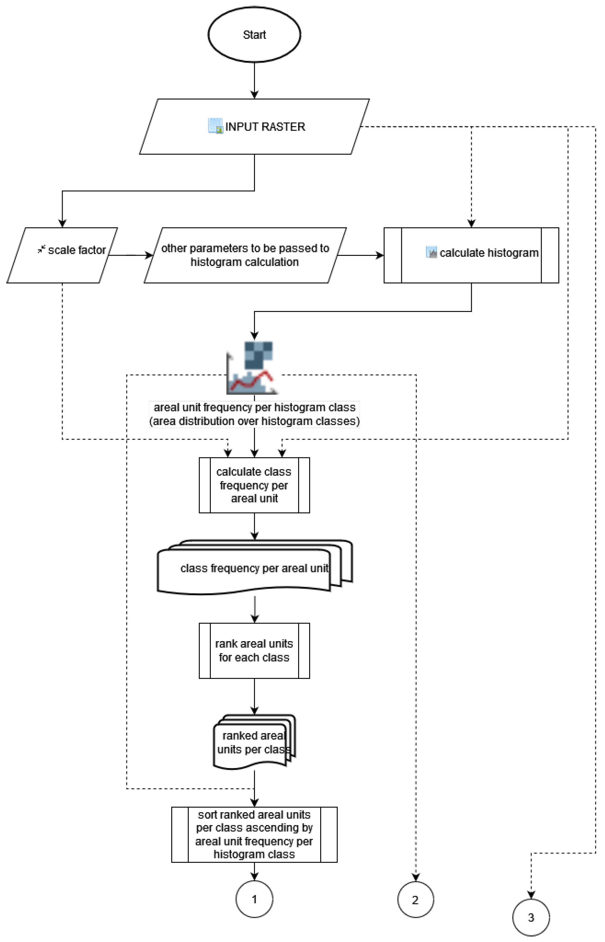
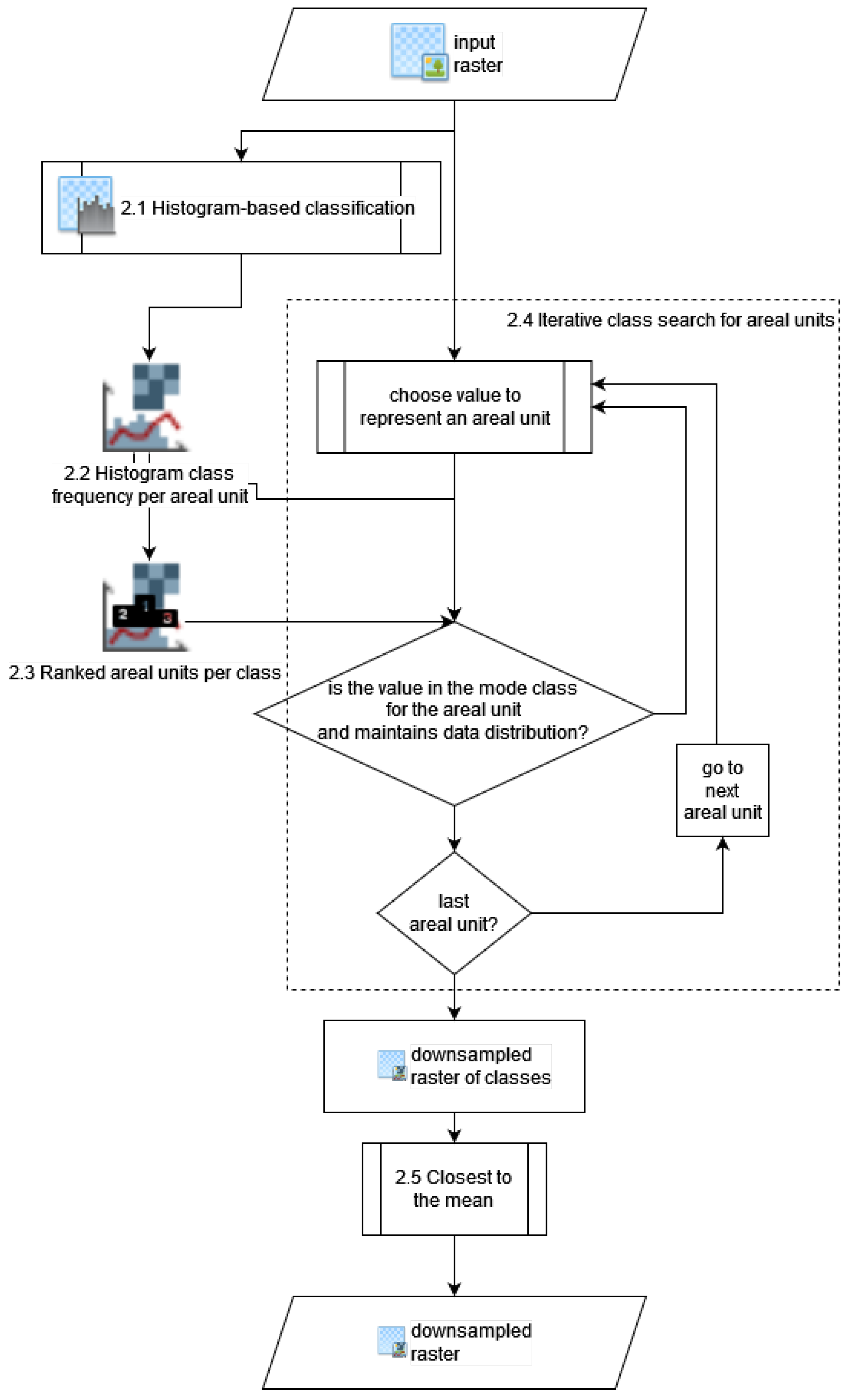
The downsampling method’s parameters are a raster image, a scale factor, and (optionally) other parameters to be passed to the histogram calculation. We present (see
Figure 1) and describing the main parts of the method. The downsampling method is also presented in more detail in the
Appendix A flowchart, split into
Figure A1 and
Figure A2.
2.1. Histogram-Based Classification
First, the histogram of the input raster is calculated. The histogram breaks are used as thresholds to calculate the histogram-based classified raster, while the count of pixel values in each bin are used to estimate the count of areal units belonging to each histogram class after downsampling. These per-class areal unit counts are later used as caps for selecting values belonging to each class.
2.2. Histogram Class Frequency per Areal Unit
The histogram-based raster classification is split into a stack of binary rasters per class, and then each raster is sum aggregated at the required downsampling scale. Each areal unit will contain a value between zero and the square of the scale factor, representing the count of values from the input image, belonging to the respective class and areal unit. This count represents the “power” of the class in the areal unit. For brevity, we will call this raster stack the power stack, similarly to how it is named in our R implementation.
2.3. Ranked Areal Units per Class
Existing power values are independently consecutively ranked per class. The highest power per class is assigned the highest rank, 1, while the lowest rank is a higher value equal to the number of existing powers inside its respective class. The power stack is then reclassified according to its rank. Ranking powers are useful because they normalize the power values, e.g., very dispersed classes, may only have low powers, but when ranked, each class will have top ranking (1) areal units.
2.4. Iterative Class Search for Areal Units
The goal in this step is to assign a class to each areal unit, giving preference to classes with a lower total count of areal units. In our R implementation, we start with an empty template based on one of the ranking rasters, which is then filled iteratively to obtain a histogram class-based downsampled raster.
In each iteration, we attempt to find the most suitable areal units to which to assign the current class, up to the cap calculated according to the histogram in the first step (see
Section 2.1).
The search follows two rules:
2.4.1. Top Ranking per Class Rule
All top-ranking areal units up to the cap per current class are considered eligible. Since there are usually more areal units with the same ranking, it may be that with the last eligible rank, there may be more suitable areal units than the cap. In this situation, we dismiss, at this step in the algorithm, the last eligible rank, and we admit all other higher ranking areal units as suitable. In our R implementation, we call this last eligible rank the edge rank. If there is no edge rank, perhaps because the cumulative count of areal units for all eligible ranks perfectly matches the cap, then we fill the template with the found areal units and move to the next class.
2.4.2. Bottom Global Rank per Subsequent Classes in the Current Class Edge Rank
If there is an edge rank, it means we did not reach the cap of needed areal units, and we consider eligible all areal units within the edge rank. The goal now is to find the areal units within the edge rank of the current class, which are least relevant for the subsequent classes. To do so, for each eligible areal unit, we calculate the top rank among all subsequent classes, called a global rank. We then consider suitable for the current class, as many areal units as needed, in descending order of the calculated global rank. After we fill these areal units as well, there are as many areal units corresponding to the current class, as dictated by the histogram of the native image, and we can move to the next class.
2.5. Closest to Mean
Ultimately, we need to obtain a downsampled raster with values from the input raster. For this, we replace class values in the histogram class-based downsampled raster with a corresponding pixel value, which is closest to the mean of all pixel values in the respective class and areal unit. This raster is returned as the output of the proposed novel downsampling method.
2.6. Multiple Bands Stack Voting
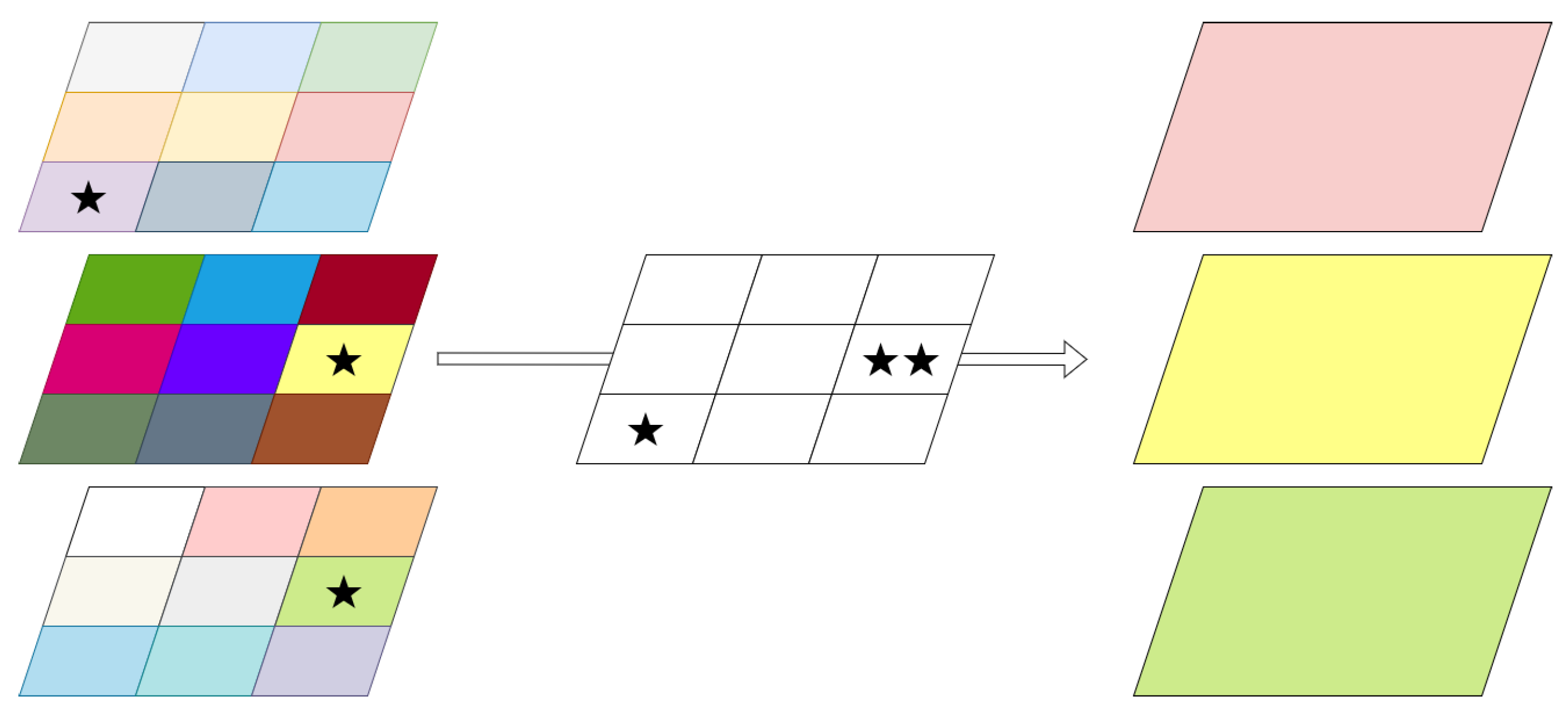
The downsampling method explained so far only applies to a single-band raster. Yet, more often than not, input rasters come in the form of multi-band rasters. Or, sometimes, multiple rasters with the same extent are used as input. If we apply the downsampling individually to each raster band, and we feed these downsampled rasters to a processing algorithm, we would most likely break the reasonable assumption that location-wise corresponding pixels are perfectly spatially overlaying. To solve this multi-band raster issue, we propose a band voting mechanism shown in
Figure 2. First, each input is downsampled accordingly. For each band, the position that is selected to represent the areal unit is recorded. Finally, the most selected positions are used for pixel selection in all bands. If there are ties within an areal unit, it does not matter which value is chosen, but in our implementation, the first in R’s indexing order is chosen.
3. Validation Case Study
3.1. Is the Novel Downsampling Better?
To assess the performance of the novel downsampling method, we compare it to traditional downsampling methods, i.e., mean, and central pixel selection. Moreover, we include it in the comparison of random downsampling. By mean downsampling, we understand that the value representing an areal unit is calculated by averaging the pixel values. By the central pixel selection, we understand that the value representing an areal unit is the value of the pixel in the center of the areal unit. In the case of evenly sized areal units, we select the top left pixel of the four pixels touching the center of the areal unit. By random downsampling, we understand that the value representing an areal unit is randomly selected from the pixels covering the aggregated areal unit. We implemented random downsampling ourselves because it is not a standard downsampling method. We included it as a lower benchmark than traditional downsampling methods. A lower benchmark might reveal some insight into the performances of traditional downsampling methods as well.
Based on the theory on which the novel downsampling is built, we hypothesize that, if downsampling of a raster dataset is needed, and there is no particular knowledge on the interactions between the downsampling method, the dataset, the downsampling level, and the processing algorithm that uses the downsampled raster as input, then the output of the processing algorithm is more likely to be improved by choosing the novel downsampling method.
3.2. Experimental Design
We propose testing the hypothesis by using the four downsampling methods in conditions similar to those used by a remote sensing user. We first downsampled a dataset, then processed the downsampled version to obtain a map. The workflow can be seen in
Figure 3.
The output map is compared to its respective non-downsampled version as further detailed. Non-downsampled output maps, which are the same as downsampling with a downsampling factor of 1, are the control results of the experiment.
The final comparison was done on locality, further defined. Locality aims to answer how well data are preserved at the same location. It is defined as the percentage of the area of the output raster, which is identical in value, by position, to the control output.
The experiment has one independent variable, three nuisance variables, and one dependent variable, as described in
Table 1. This experimental design is more properly described as two concomitantly run sub-experiments, for each remote sensing application.
Table 1.
Experimental design.
Table 1.
Experimental design.
| Variable | Type | Cardinality | Levels | Sampling Strategy |
|---|
| Downsampling method choice | Independent | 4 | Novel mean central random | N/A |
| Remote sensing application | Nuisance | 2 | bfast random forest | Judgment |
| Raster datasets | Nuisance | | Figure 4 | Judgment sampling |
| Downsampling factors | Nuisance | 9 | 2 to 10 | Judgment sampling |
| Locality | Dependent | Continuous | N/A | N/A |
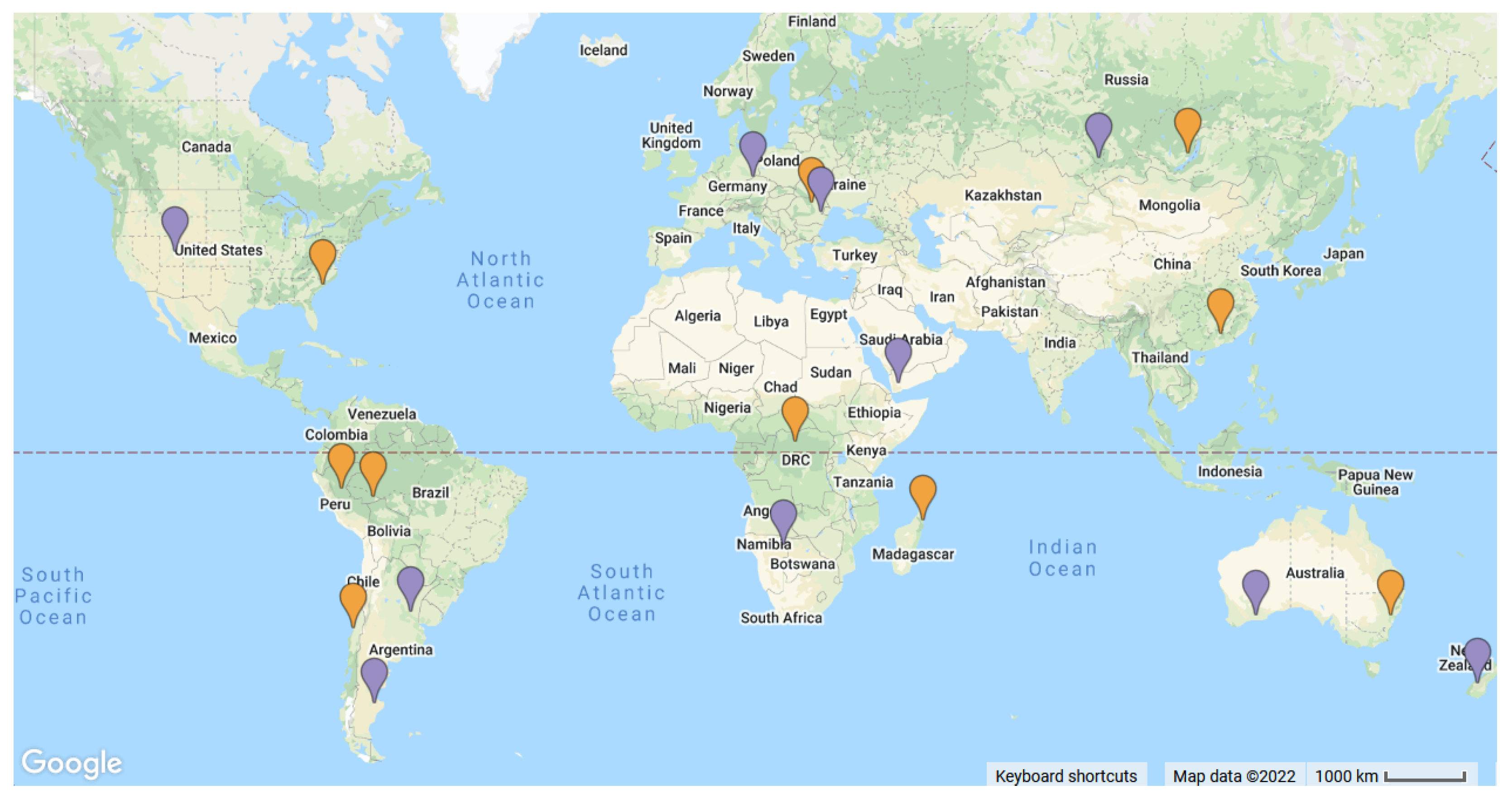
Figure 4.
Locations of datasets used as input for bfastmonitor (orange) and random forest (purple).
Figure 4.
Locations of datasets used as input for bfastmonitor (orange) and random forest (purple).
3.3. Nuisance Variables
When downsampling, a change in the downsampling factor, the dataset, or the remote sensing algorithm is likely to change the locality of the output maps. We did not consider these variables to be independent, but nuisances. We did not try to observe their effects, but just the effect of the downsampling method choice. By varying the downsampling factor, the dataset, and the remote sensing algorithm, we attempted to increase the variation of the dependent variables in order to increase the robustness of the experiment.
3.3.1. Downsampling Factors
We speculate that most users are interested in downsampling as little as possible or necessary, so we tested the downsampling methods at the nine different consecutive downsampling factors closest to no downsampling, further detailed. The limits of the nine downsampling factors were arbitrary and made out of convenience to limit the size of the experiment. For brevity, we further reference the 9 downsampling factors (of 2 to 10) as the 10 downsampling factors of 1 to 10. In the framework of this experiment, a downsampling factor of 1 is the same as not downsampling, resulting in control output maps.
3.3.2. Datasets
We ran each remote sensing processing algorithm sub-experiment on 10 datasets each (
Figure 4). Similarly, the decision to limit ourselves to 10 datasets each was made out of convenience and to limit the size of the experiment.
The size of each dataset was chosen so that at the highest downsampling factor of 10, there would still be 100 by 100 pixels left in the dataset. The locations of these datasets were chosen only considering criteria that would make sense for non-trivial results, with respect to the chosen processing algorithm. More specifically, for bfastmonitor, we excluded all primary forest and non-forested areas, in line with a typical bfastmonitor analysis. For the random forest-based land cover classification analysis, we dismissed obviously homogeneous locations, such as deserts. The sources of all datasets were Landsat 8 scenes and Copernicus Global Land Cover Layers (Collection 2) [
27] as labels.
The choice of data source had« to be usable for our chosen processing algorithms. As bfastmonitor is typically run on a time series of indexed data, such as Normalized Difference Moisture Index (NDMI), we had to choose a data source with the necessary bands and typical usage time frequency. The two most popular data sources with these specifications were Landsat and Sentinel 2. We chose Landsat 8 because its surface reflectance products are always immediately available on Google’s Earth Engine Data catalog, which was only partially true for Sentinel 2 data at the time of processing. Of course, the downsampling itself is agnostic to the differences between these two data sources, such as specific wavelengths, or how the imagery has been rectified. The downsampling method is even agnostic to the difference in resolution between Landsat 8 and Sentinel 2. From the downsampling method point of view, a factor of 1 means native scale, regardless of whether that means 10 or 30 m on the ground. The difference in resolution between data sources must be considered a change in sampling. Since we already tested across different scales, and downsampling is agnostic to any other difference, we only used Landsat 8 as the data source, as it completely covers all of our research goals.
3.3.3. Processing Algorithms
We limited the factors of the remote sensing processing algorithm to only two levels, i.e., bfastmonitor [
28] and random forest [
29] land cover classification, to limit the size of the experiment. In the following paragraphs, we will describe bfastmonitor for deforestation monitoring and random forest for land cover classification. Out of all possible processing algorithms, we sampled these two processing algorithms by convenience sampling. The factors we took into consideration for convenience sampling were the ease of use for the researchers performing the experiment, availability, and perceived popularity. These algorithms are typically run on disjunct datasets; we also split our experiment into two (identically set up, but technically separate) sub-experiments.
Bfastmonitor is a popular remote sensing algorithm, often used for forest monitoring. Bfastmonitor works on a time series split into a historical and a monitoring period. The historical data were used to determine a stable signal against which abrupt changes were detected in the monitoring period. We used the Python implementation [
2] with default parameters, except for
k (harmonics) and the
. The only deviation from default bfastmonitor parameters is that we used
and
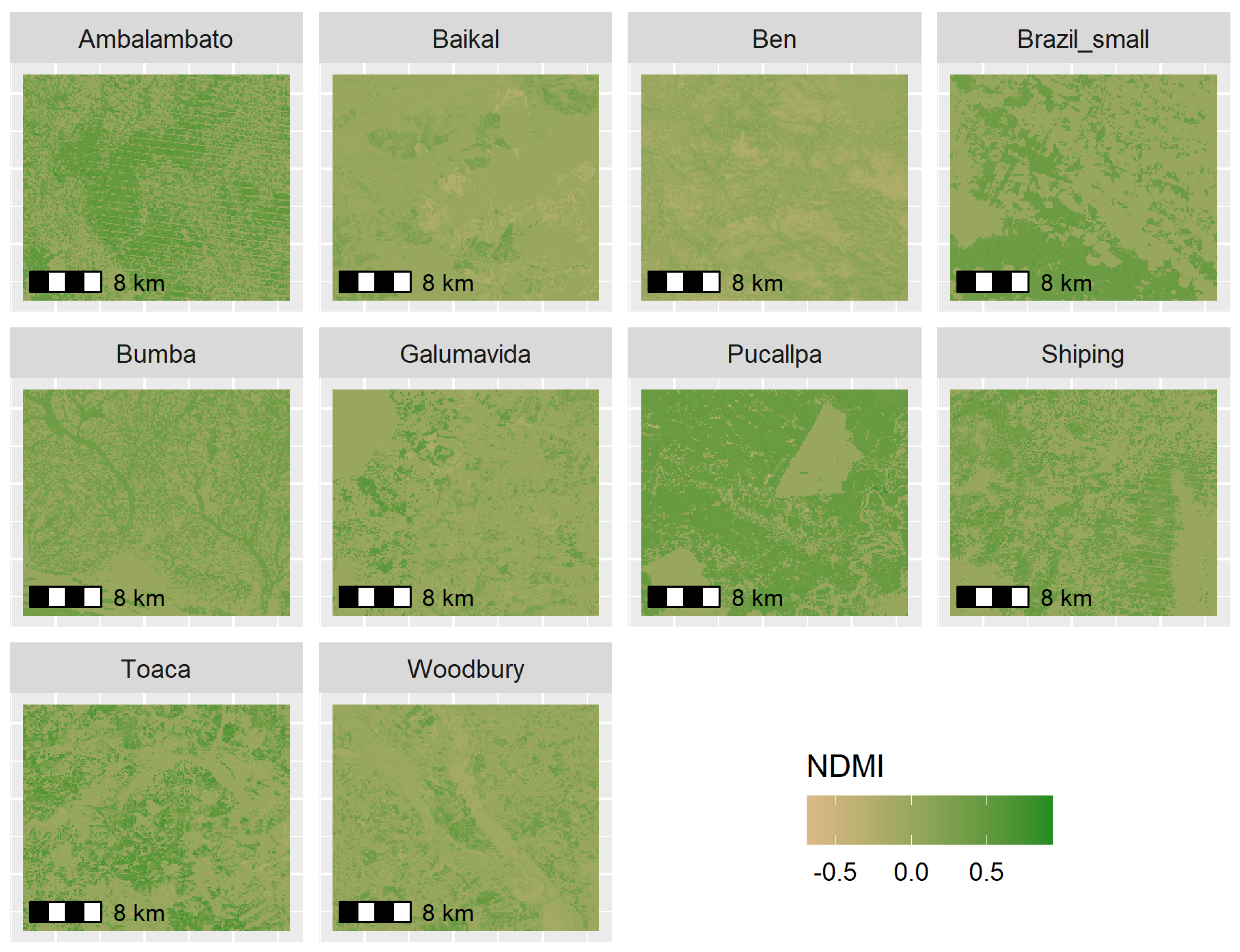
because we appreciated that it was the more used (and faster) scenario, yet we would not expect different results from this experiment regardless of the choice of bfastmonitor parameters. From our experience, bfastmonitor parameters are incrementally tuned to fit the particularities of the dataset it is run on. The datasets used as input for bfastmonitor were the NDMI time series spanning 10 years (from 2010 to 2020). The most recent layers of these time series are presented in
Figure 5.
Random forest is a classification method that outputs the most popular class selected by an ensemble of decision trees. Random forest is a popular algorithm used in the remote sensing field for land cover classification. We used the Python implementation [
30] with default parameters, except for
. We fixed
for reproducibility (and because it is a popular scenario). We used the Copernicus Global Land Cover Layers (Collection 2) [
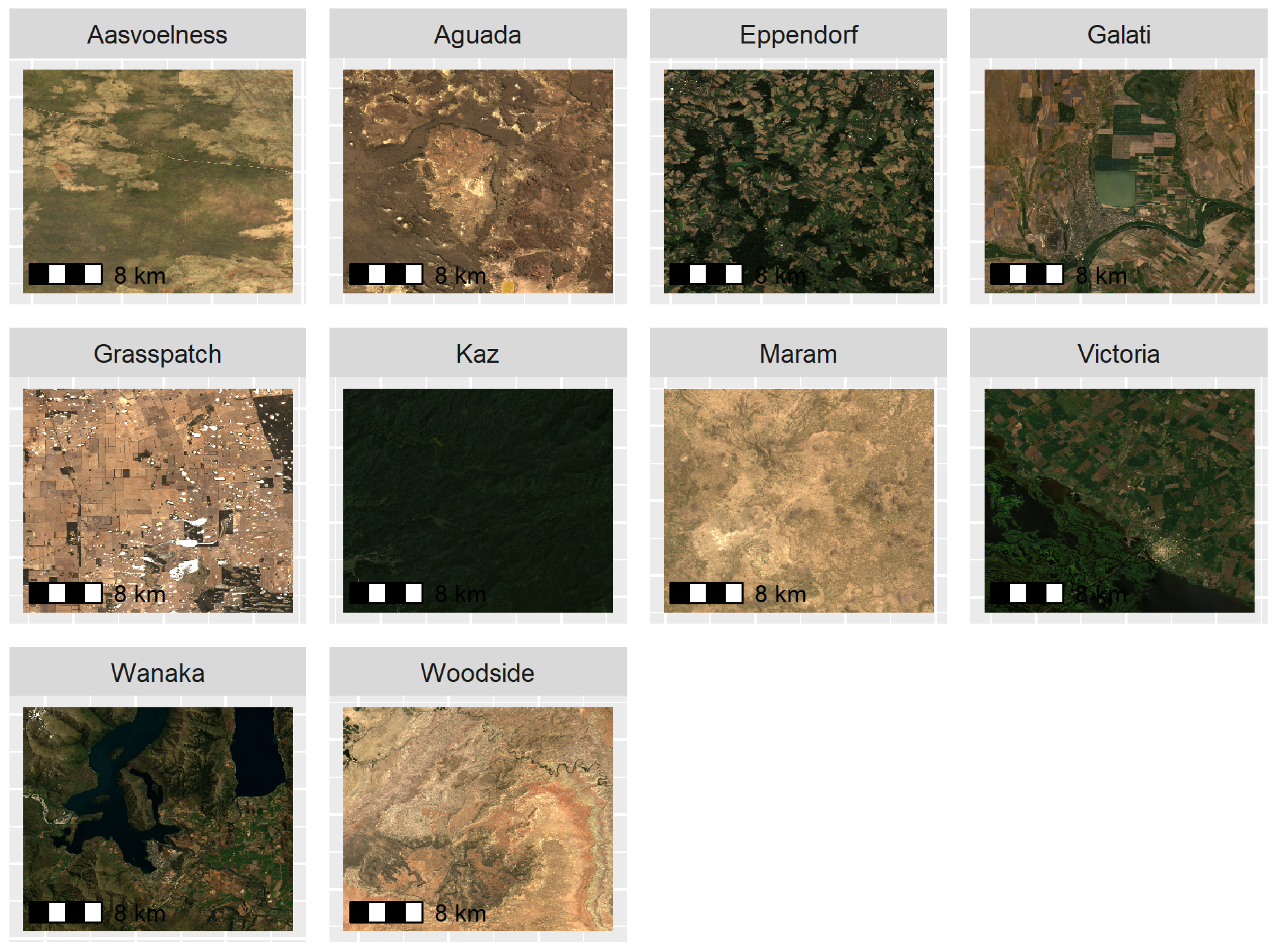
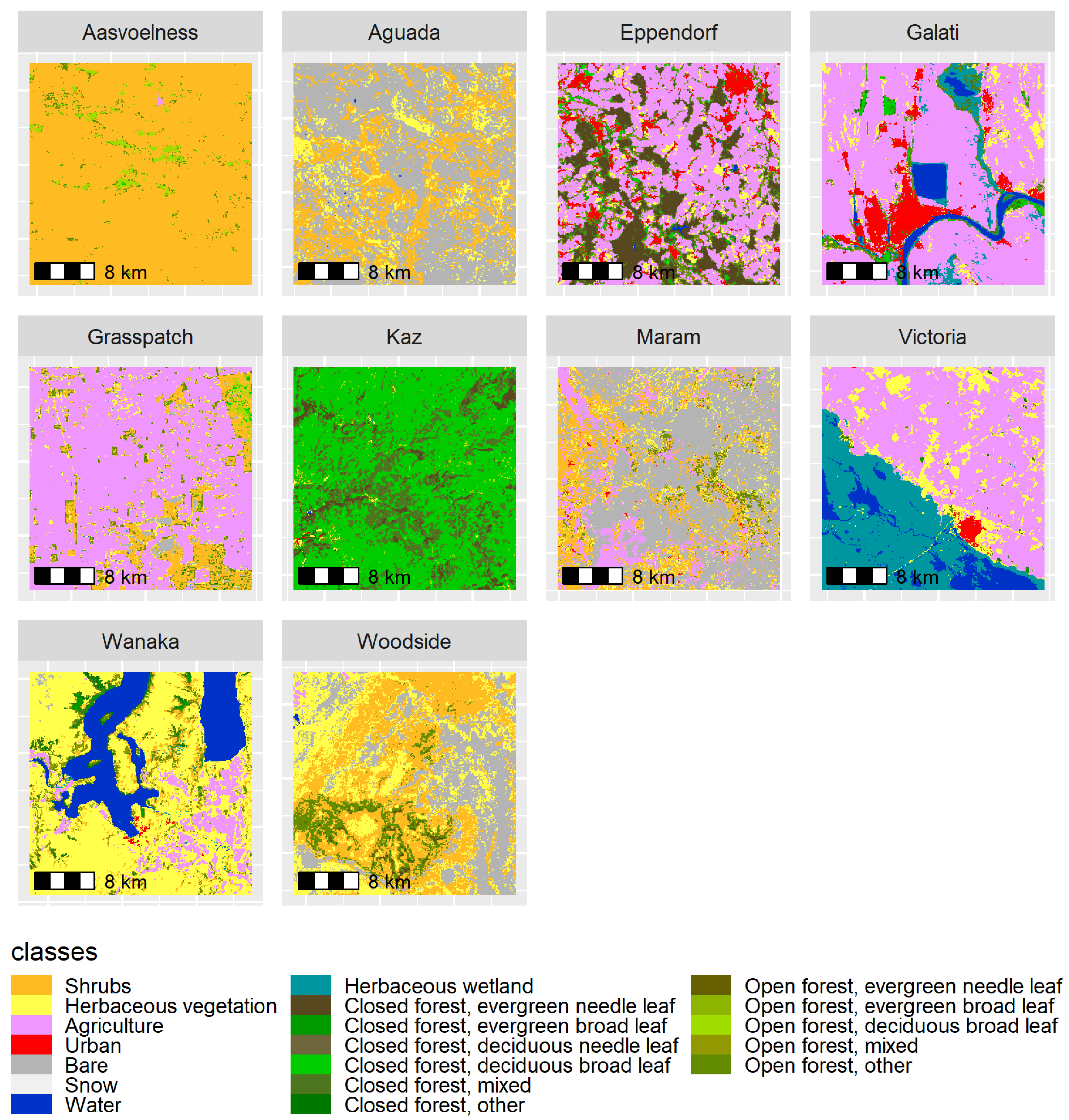
27] to train the random forest model. For each area, we randomly selected 100 points to train the model on Landsat 8 imagery (
Figure 6) and Copernicus Global Land Cover Layers, as labels (
Figure 7). The model was not trained on a time series of Landsat 8 imagery, but on all surface reflectance bands of a single recent Landsat 8 image, for each area, which met the following criteria, which we considered typical for the tested scenario. We chose the first cloud-free (maximum 1% cloudiness) summertime Landsat 8 scene. For summertime, we selected the months January, February, and March for the southern hemisphere, and July, August, and September for the northern hemisphere.
Both bfastmonitor and random forest had parameters that were typically fine-tuned to the target dataset before the final run. Although our intention was to test the downsampling methods as they would be used in an end-to-end production processing chain, we skipped this parameter-tuning step for two reasons. Firstly, the scale of the experiment would increase significantly. Secondly, we were not interested in the absolute accuracy of the results. Therefore, we ran the algorithms using the same parameters on each location under the assumption that the variation of our dependent variable did not depend on this fine-tuning step.
3.4. Experiment Results Analysis
We used the R stat implementation of the Wilcoxon paired signed-ranks [
31] test to assess whether the localities were significantly different.
We had no knowledge about the distribution of the calculated metrics. Aliasing, or other specific arrangements, may skew the distributions of these metrics. This lack of knowledge about the distribution of the dependent variable reduces the robustness of relying on averages of scores as a means to quantify and understand the differences between the scores obtained by using each downsampling method. For the same reasons, the popular t-test would not be as reliable in the lack of normality.
The Wilcoxon paired signed-ranks test brings evidence (or disproves) that a downsampling method is more likely to yield a better result when it comes to our dependent variables. Considering that remote sensing users usually have to pick a downsampling method without much knowledge about interactions between their remote sensing algorithm, their dataset, and the downsampling factor, or method, we find this test relevant in assessing the results of this experiment. We used the traditional significance level
[
32], due to its ease of understanding, but also because we believe remote sensing users are not ‘interested’ in being more than 95% sure about which downsampling method to choose.
5. Discussion
Geocomputing platforms, such as Google Earth Engine [
5], use downsampling as part of image pyramid building to handle large volumes of data on the fly (and at appropriate scales). Google Earth Engine follows conventional wisdom and uses mean and first value (translated central pixel selection) downsampling as default pyramiding policies for continuous and discrete-valued images, respectively. Mode, min, and max are also available as options for user-uploaded datasets. A scenario we often encounter is estimating discrete classes as fractions at a lower scale. Since it is a discrete-valued dataset, either sampling the first value, mode, min, or max would be used. The obvious solution is to calculate the fractions based on the native resolution imagery, but that is likely to be computationally expensive and it does not leverage the image’s pyramid, which is the core strength of using a geocomputing platform. Alternatively, fractions could be estimated from an image midway in the pyramid between the native resolution and the targeted scale. The midway strategy would lead to biased results under min, max, and mode towards the min, the max, and the most frequent class, respectively. The default first value sampling pyramiding policy would also be biased towards the most frequent class, but it would also have an extra error depending on aliasing. This indicates that specific use cases cannot be effectively handled with conventional downsampling methods, such as pyramiding policy. The presented novel downsampling method would allow the usage of the midway strategy with a minimal error proportional to the distance between the native and the chosen midway level in the pyramid. The novel downsampling method is also likely to improve the results for many other use cases as well, with the only minor disadvantage of additional computation costs at the data ingestion moment, which should be easily offset by all the computations done on the image dataset.
The novel downsampling method is more expensive in terms of processing. Of course, downsampling an input should only be performed when downsampling costs are marginal compared to actual processing costs. Therefore, if the user knows before processing that they are not interested in the output data distribution, then the central method downsampling might be better due to lower processing costs. If the user is unsure about which characteristics of the output they are interested in, the novel downsampling method provides similar or better scores for the locality as central, while presumably maintaining output data distribution.
The proposed novel downsampling method is just one possible solution to tackle the modifiable areal unit problem. Our method is based on a few basic principles, such as spatial autocorrelation and people’s tendencies to classify objects based on how much the basic components are alike, e.g., ‘more trees’ is a forest, and ‘more corn’ is a crop. Our work follows the suggestions from Xu et al. and provides an important step in tackling the modifiable areal unit problem, as it affects remote sensing, but we did not find an optimal solution. Since solving the modifiable areal unit problem is the same as solving representativity in representative democracies, we believe an optimal solution may not exist. Nevertheless, not all suboptimal solutions are equal and potential other avenues exist to address the modifiable areal unit problem. We envision that future research could focus on application specific downsampling.
We hope the remote sensing research community will be interested in testing our downsampling method, or other downsampling methods, in various scenarios applicable to their workflow. We recommend not focusing on how downsampling affects different data sources alone, e.g., comparing the effects of downsampling on similar products obtained from MODIS, LANDSAT, and Sentinel 2. Such an experiment would first and foremost describe the differences in resolution between the three datasets. If the goal of the experiment is to compare downsampling on datasets at different scales, we would recommend choosing a single dataset to avoid misattributing scale effects to wrong variables, such as the data provider. Instead, we suggest an experiment that compares the effects of using our downsampling method in combination with many other processing algorithms.
Further, once our downsampling method is independently validated, we suggest integrating our downsampling method with other remote sensing big data solutions, such as moving processing into the cloud [
4,
5]. While downsampling is already implemented in pyramid policies, a better downsampling, such as ours, would improve the quality of pyramid-based processing. We believe that global scale monitoring applications, such as deforestation monitoring [
9,
10,
11], would improve by using our downsampling method. Our most prominent current issue (for which we desire future work to focus on) is our ‘sloppy’ research, such as implementation that is to never be fixed by the engineering community.
