Article

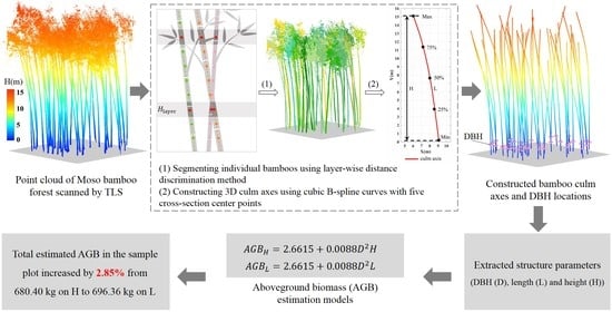
Refined Aboveground Biomass Estimation of Moso Bamboo Forest Using Culm Lengths Extracted from TLS Point Cloud

1
Chongqing Jinfo Mountain Karst Ecosystem National Observation and Research Station, School of Geographical Sciences, Southwest University, Chongqing 400715, China
2
Chongqing Engineering Research Center for Remote Sensing Big Data Application, School of Geographical Sciences, Southwest University, Chongqing 400715, China
*
Author to whom correspondence should be addressed.
Remote Sens. 2022, 14(21), 5537; https://doi.org/10.3390/rs14215537
Submission received: 28 August 2022 / Revised: 17 October 2022 / Accepted: 1 November 2022 / Published: 3 November 2022
(This article belongs to the Special Issue Terrestrial Laser Scanning of Forest Structure)

Abstract

:
Bamboo forest is a special forest type, and its aboveground biomass (AGB) is a key indicator of its carbon sequestration capacity and ecosystem productivity. Due to its complex canopy structure and particular growth pattern, the AGBs of individual bamboos that were estimated using traditional remotely sensed data are of relatively low accuracy. In recent years, the point cloud data scanned by terrestrial laser scanners (TLS) offer the possibility for more accurate estimations of bamboo AGB. However, bamboo culms tend to have various bending degrees during the growth process, which causes the AGB estimated on culm height (H) to be generally less than the true value. In this paper, taking one sample plot of the Moso bamboo forest in Hutou Village, Chongqing, China as the study site, we employed a TLS to acquire the point cloud data. The layer-wise distance discrimination method was first developed to accurately segment individual bamboos from the dense stand. Next, the diameter at breast height (DBH) and culm length (L) of an individual bamboo were precisely extracted by fitting the cross-section circle and constructing the longitudinal axis of the bamboo culm, respectively. Lastly, the AGBs of the Moso bamboos in the study site were separately calculated using the allometric equations with the DBH and L as predictor variables. As results, the precision of the complete bamboo segmentation was 90.4%; the absolute error ( A E ) of the extracted DBHs ranged from −1.22 cm to 0.88 cm ( R 2 = 0.93, R M S E = 0.40 cm); the A E of the extracted Hs varied from –0.77 m to 1.02 m ( R 2 = 0.91, R M S E = 0.45 m); and the A E of the extracted Ls varied from −1.08 m to 0.77 m ( R 2 = 0.95, R M S E = 0.23 m). The total estimated AGB of the Moso bamboos in the sample plot increased by 2.85%, from 680.40 kg on H to 696.36 kg on L. These measurements demonstrated the unique benefits of the TLS-acquired point cloud in characterizing the structural parameters of Moso bamboos and estimating their AGBs with high accuracy.

Graphical Abstract

1. Introduction

Bamboo forests are a special forest resource widely distributed in South and Southeast Asia [1]. Approximately 15% of the world’s bamboo forests are concentrated in China [2], covering an area of 6.52 million ha [3]. As a major bamboo species, Moso bamboo (Phyllostachys pubescens) accounts for approximately 74% of the total bamboo area in China [4]. Compared with those timber trees, Moso bamboo has a unique growth and reproduction system. It takes approximately two months to grow from the unearthed shoots to the young bamboos [5]. With the advantages of rapid growth, widespread distribution, and a strong carbon sequestration capacity relative to other plant species, Moso bamboo has made a significant contribution to the global carbon balance [5]. As one of the important quality parameters of terrestrial ecosystem, the aboveground biomass (AGB) of vegetation, including Moso bamboo forest, is a key indicator for estimating carbon reserves [6,7,8,9].
In recent years, various remotely sensed data have been used to extract forest structural parameters and quantitatively estimate forest AGB [10]. Due to the complexity of the bamboo canopy and the particularity of the growth pattern, traditional passive remote sensing techniques were relatively limited in obtaining bamboo canopy structure. In contrast, as an active remote sensing technology, Light Detection and Ranging (LiDAR) can continuously emit laser pulses, which are capable of penetrating the bamboo canopies to capture the three-dimensional (3D) structure and the topographic information under the canopies [11]. Among them, airborne laser scanning (ALS) has obvious advantages in forest parameter extraction on a large scale, but generally cannot obtain detailed canopy information [12]. In contrast, terrestrial laser scanning (TLS) can even record forest branches and foliage (B&F), making it possible to the acquire forest structure parameters with high precision. Recently, researchers have achieved fruitful results in extracting forest parameters using TLS [13,14]. For example, TLS was widely used to extract basic forest parameters such as tree height [15,16,17], diameter at breast height (DBH) [18], individual tree position [19], leaf area index (LAI) [13], and so forth.
Tree segmentation is the basis of extracting individual tree structure parameters from the LiDAR point cloud. Many researchers have proposed solutions and algorithms in this regard. In earlier developments, most of the segmentation algorithms followed the steps of first identifying the tree trunk positions, and then allocating crown points to the respective trunks [16,20]. Maas et al. [21] used vertical cylinders to separate the point cloud of individual trees by detecting tree trunk positions. Cabo et al. [17] projected the point cloud onto a 2D plane, and segmented the single trees by constructing a Voronoi diagram. However, the previous two methods can only work well in open forests with sparsely distributed trees. Under complex forest conditions, understory shrubs and interlaced B&F will have a significant impact on segmentation. Hence, several methods focusing on crown segmentation were presented recently. Tao et al. [22] developed a comparative shortest-path algorithm that helped to assign points in the intersection area to the corresponding trees. Wang et al. [14] proposed a graph pathing algorithm to achieve point-wise canopy segmentation. Xing et al. [23] applied the layer-by-layer clustering method to trees with irregular canopy shapes, achieving fair results in a plantation forest, and the method has also been widely applied in studies such as branch separation [24]. In recent developments, deep learning has been gradually applied to individual tree segmentation [25], and has made some exciting progress. Nevertheless, accurate individual bamboo segmentation remains challenging in stands with heavy canopy intersections and bent culm forms.
Although direct destructive measurements are the most accurate way to obtain AGB [26], they may cause irreversible damage to forest ecosystems [27]. Indirect measurements of forest biomass are generally achieved using allometric models, with the tree height and DBH used as predictor variables [15,28]. In the field work, the forestry staff usually use the clinometer and DBH ruler to measure heights and DBHs of individual trees, respectively. Due to the occlusion of neighboring canopies in dense stands, it frequently happens that the clinometer cannot be accurately pointed to the treetops. This also occurs in the height measurement of bamboos with high density. In contrast, as the point cloud scanned by TLS is of an ultra-high density, the subtle morphological features of bamboos can be detected, enabling the bamboo heights (H) and DBHs to be accurately extracted [29]. In general, the bamboo height is referred as the difference between the maximum and the minimum elevation values of the point cloud of an individual bamboo [17]. However, bamboo culms tend to have varying degrees of bending during the growth process; hence, the culm heights are commonly shorter than the culm lengths. As a result, the bamboo AGBs estimated on their heights are generally less than the true values.
In this study, we aimed to extract the culm lengths (L) of individual Moso bamboos from the point cloud scanned by TLS, and then use them to replace the culm heights to achieve more accurate AGB estimation. The major contributions include: (1) developing an algorithm to accurately segment and extract the point cloud of individual Moso bamboos in a dense stand; (2) realizing the automatic construction of the longitudinal axis of the bamboo culms, and calculating their lengths using mathematical integration; and (3) using the allometric equation with the DBH and bamboo culm length as predictor variables to achieve a refined AGB estimation of individual Moso bamboos.

2. Study Site and Data

2.1. Study Site

As shown in Figure 1a, the study site (29°44′18″N, 106°18′22″E) is located in Hutou Village, south-west of Chongqing City, China. It is situated at one hillside with elevations ranging from 337.64 m to 722.31 m. This region is characterized by a humid subtropical monsoon climate with a mean annual temperature of 18 °C and a mean annual rainfall of 880 mm. The major forest types include coniferous forest, broad-leaved forest, and bamboo forest, and the tall plant species are Moso bamboo, Osmanthus fragrances, fir, and Bambusa multiplex. As indicated in Figure 1b, a sample plot of Moso bamboo forest with an area of 8 × 12 m was selected as the study object. In the plot, the culms of Moso bamboos exhibit varying bending degrees. Therefore, it is an ideal study site for accurately estimating the AGBs of individual Moso bamboos by extracting their culm lengths.

2.2. Point Cloud Data

The 3D point cloud data of the sample plot was acquired by FARO Focus S350 (FARO Technologies, Inc., Lake Mary, FL, USA). The instrument is a high-speed 3D laser scanner with a measurement distance ranging from 0.6 m to 330 m. Its vertical field of view (FOV) is 300°, and its horizontal FOV is 360°. The working laser wavelength is 1550 nm, and the ranging error is 1 mm. The laser scanning operations were carried out on 24 December 2021. Before scanning, six registration spheres were reasonably placed in the plot, ensuring that at least three common spheres were visible from each pair of neighboring scanning positions [18]. Then, four scanning stations were sequentially set around the sample plot of Moso bamboos to allow the laser pulses to reach the bamboo tips as far as possible, and finally, the raw point cloud data were obtained.
After field work, the raw point cloud data were first registered using the affiliated software SCENE 7.0 (Figure 2a). As shown in Figure 2b, the point cloud was then cropped to ensure the integrity of the individual Moso bamboos. The point number of the resulting point cloud was further reduced using the random sampling algorithm [30], and the point outliers were removed using the StaticalOutlierRemoval algorithm [31]. Next, the cloth simulation filter [32] was used to separate the ground points from the bamboo points (Figure 2c). Lastly, the values on the Z-axis of the bamboo points were normalized from altitudes relative to the sea level to heights relative to the ground (Figure 2d). All of these preprocessing functions were directly executed in CloudCompare 2.14, an open source point processing tool. The preprocessed point cloud data of the sample plot of Moso bamboos is shown in Figure 1c.

2.3. Measured Data

After the TLS scanning operations, a field survey was also carried out on the study site, and there were 42 Moso bamboos identified in the sample plot. The DBHs of individual Moso bamboos were measured with a DBH ruler at a height of 1.3 m above the ground. The Hs were measured using a total station Nikon DTM-352c, and the instrument height was set to 1.55 m. The height angles and horizontal distances of individual Moso bamboo were measured, and their heights were then calculated using trigonometric leveling. Due to the various bending degrees of the Moso bamboos, it was difficult to measure the Ls in the field. Instead, the points of individual Moso bamboos were manually separated in CloudCompare, and their Ls were also manually measured using the measuring tool provided in the software. The statistics of measured DBHs, Hs, and Ls of individual Moso bamboos in the study site were listed in Table 1.

3. Methods

3.1. Individual Bamboo Segmentation

As TLS scans point cloud in a bottom-up mode, the tree segmentation algorithms generally follow a similar approach [16,20]. The stem points are first identified and then expanded to those of B&F. However, these algorithms do not work well for a dense bamboo forest with interlaced culms and B&F. In the study, we developed a bamboo segmentation algorithm that enabled the precise extraction of individual bent-grown Moso bamboos. It mainly consists of two steps: the seed point generation and the individual bamboo segmentation through layer-wise distance discrimination.

3.1.1. Seed Point Generation

As shown in Figure 3a, the seed points for individual bamboo segmentation are selected in the horizontal point strip cut out from the bamboo culms. To eliminate the influence of low vegetation, the upper limit and lower limits of the point strip are determined as 3 m and 1 m, respectively. The seed points for bamboo culms are generated on the fact that the culm points and B&F points have different spatial distribution and geometric characteristics [26]. The Moso bamboo culm has a flat surface, so its points tend to have a local smoothness. In a sufficiently small region, the culm points are approximately distributed on the same plane. Hence, the k-NN (k-nearest neighbor) method (Equation (1)) is used to find the neighbor points of each point in the strip for the covariance matrix analysis ( C o v p ), and the geometric features of the point cloud will be constructed based on the combination of eigenvalues and eigenvectors [26,33]
C o v p = i = 0 k p i p ¯ p i p ¯ T k
where p i = x i , y i , z i T is a 3D point and p ¯ is the central point of the k nearest neighbor points.
The B&F points are removed as much as possible based on the geometric features, including surface variation (SV) (Equation (2)) and verticality (V) (Equation (3)). The remaining culm points are to identify the positions of the individual Moso bamboos (Figure 3b), and then are clustered to generate the seed points at 1.3 m (Figure 3c).
SV = λ 1 λ 1 + λ 2 + λ 3
V = Z × n
where 0 λ 1 λ 2 λ 3 are the eigenvalues of the covariance matrix; Z = 0 , 0 , 1 , and n denotes the normal vector.
The SV is used to quantify the change in the surface where the points are located. The higher the SV, the more drastic the change. The V is used to describe the spatial relationship between the surface where the points are located and the horizontal plane. The low value of V means that the points are on a vertical structure [34].

3.1.2. Layer-wise Distance Discrimination

After the seed point generation, the individual Moso bamboos are segmented using layer-wise distance discrimination (LDD). The point cloud is first sliced into a series of horizontal and successive layers, and the layer thickness is denoted as H l a y e r . Theoretically, as long as the layers are thin enough, the points of neighboring layers belonging to the same bamboo are approximately within a minimum range of the same vertical line. Then, the point cloud of a single bamboo is divided into two parts by the under-branch height ( H u b ). The point cloud below H u b is taken as the culm point and that above H u b as the canopy point (Figure 4a). The culm points are layer by layer segmented using the clustering center of layer L i to cluster the points of layer L i and generate the clustering center of layer L i + 1 (Figure 4c), whereas the canopy points are segmented using the clustering center of layer L j 1 to cluster the points in layer j and generate the clustering center of layer L j (Figure 4b). The process can be summarized as follows:
(1)
The layer L s , where the seed points are located, is taken as the starting layer, and the seed points are used as the initial clustering centers. The distances between one target point and the seed points are separately calculated. The target point is classified to the cluster with the shortest distance, and the ID of the seed point is also assigned to it.
(2)
Radius filtering is performed on the points with the same ID to weaken the influence of outliers on the subsequent generation of clustering centers. Then a convex hull is constructed and its centroid x i , y i , z i is calculated [35]. In order to prevent the centroid from being seriously deviated, it is necessary to set constraints on x i and y i . If the distance between the obtained centroid and the clustering center is less than the threshold value in the x-y plane, the midpoint replaces the original centroid; otherwise, the clustering center is used instead. Through repeated experiments, the threshold value is determined as 0.15 m to achieve good results. The modified point x i , y i , z i + H l a y e r is used as the clustering center in layer L i + 1 . The same steps are performed layer by layer until the layers of the culm points are all handled (Figure 4c). The culm points below the seed point are treated in a similar way.
(3)
Different from the culm, the B&F of the canopy tend to grow upwards with a large inclination. This property makes it more advantageous to use the clustering center of layer L j 1 for clustering the points in layer L j . The specific process can refer to the previous steps 1 and 2, but the difference is that the modified point x j , y j , z j is used as the clustering center of layer L j + 1 (Figure 4b). Likely, the canopy points with the same IDs will be assigned to the same clusters.
(4)
All points with the same ID, including canopy and culm points, will be combined as the point cloud of an individual Moso bamboo.

3.2. Construction of Bamboo Culm Axis

The bamboo culm axis is a 3D continuous curve fitting the longitudinal form of the culm. The construction of this curve is realized via three steps: separating the bamboo culm points and the B&F points; extracting the cross-section center points layer by layer; and constructing the bamboo culm axis with cubic B-spline curves.

3.2.1. Culm Point Separation

Bamboo culm is significantly different from B&F in shape and size. In contrast to the disordered B&F points, the bamboo culm points are linear in character and have a relatively uniform density distribution. Therefore, the point cloud of bamboo culm can be separated based on these features. First, the segmented point cloud of individual Moso bamboo is horizontally layered with a thickness of 0.2 m [24] to reduce the complexity of the canopy structure (Figure 5a). Secondly, each layer of point cloud is clustered by k-NN to generate multiple point clusters. Then, the random sample consensus (RANSAC) [36] is used to detect the straight line of each point cluster (Figure 5b). The straight line length for detecting a single point cluster was determined to be at least 0.15 m through repeated experiments with various parameters. If the number of points within the straight line scope is not less than 80% of the point number in the cluster, the point cluster will be classified as bamboo culm points. Finally, all layers of the bamboo culm points are merged. The separated bamboo culm points and canopy points of the sample Moso bamboo are shown in Figure 5c,d, respectively.

3.2.2. Extraction of Cross-section Center Points

The construction of the bamboo culm axis relies on the layer-wise extraction of cross-section center points. As the cross-section shape of a bamboo culm is very close to a circle, it can be extracted using RANSAC circle fitting, and thus the center point can be conveniently obtained. In practice, however, the bamboo culm points are usually interlaced with the B&F points in the canopy. As shown in Figure 5c, there exist some parts of the bamboo culm with less points or even no points called “broken point”. For these parts, it is difficult to obtain the cross-section center points via circle fitting. To handle this situation, the layer that contains a broken point should be first located by checking the point number of each layer along the bamboo culm from bottom to top. If the point number of a layer is less than 50% of the mean value, it will be determined as the broken point layer. Then, the entire bamboo culm will be divided into two parts by this layer (Figure 6a), where the cross-section center points will be separately extracted in two different ways. Above the layer, the radius filtering is first applied to reduce the point outliers of each layer, and then, the convex hull containing the rest points in the layer is created and its centroid will be taken as the cross-section center point (Figure 6b). Below the layer, the cross-section center points of each layer are acquired using the RANSAC circle fitting (Figure 6c). In addition, the diameter of the cross-section circle at 1.3 m is extracted as the DBH of the Moso bamboo, which will be used for its AGB estimation in Section 3.3.

3.2.3. Culm Axis Construction

The culm axis is defined as a longitudinal curve in the center of a Moso bamboo culm [37]. It is actually a continuous curve in the 3D space, which can reflect the true length of the bamboo culm. As the line segment fitting is rather stiff, the B-spline curves are used to aptly characterize the longitudinal form of the bent bamboo culm. They are capable of fitting points in a segmented and smooth manner, and have the advantage of local control [38]. The five cross-section center points located at the minimum, 25%, 50%, 75%, and the maximum culm height of an individual Moso bamboo are selected as feature points to construct a 3D culm axis using cubic B-spline curves (Figure 6d).
A B-spline curve with k -degree is defined as follows [39]:
P u = i = 0 n P i N i , k u 1 k n
where P i are the control points; and N i , k u are B-spline basis functions of degree k , which are defined as follows:
N i , 0 u = 1     u i u u i + 1 0     o t h e r w i s e
N i , k u = u u i u i + k u i N i , k 1 u + u i + k + 1 u u i + k + 1 u i + 1 N i + 1 , k 1 u
where u i ,   i = 0 ,   1 ,   2 ,   , n + k + 1 are the knots, and u i u i + 1 ; U = u 0 , u 1 , u n + k + 1 is the knot vector. When k = 3 , i = 0 ,   1 ,   2 ,   3 , the basis function is as follows:
N 0 , 3 u = 1 3 ! 1 u 3 N 1 , 3 u = 1 3 ! 4 6 u 2 + 3 u 2 N 2 , 3 u = 1 3 ! 1 + 3 u + 3 u 2 3 u 3 N 3 , 3 u = 1 3 ! u 3
Therefore, the cubic B-spline equation is as follows:
C u = i = 0 3 P i N i , 3 u 0 u 1
As mentioned above, the bamboo culm axis has been divided into four curve segments, whose lengths will be separately calculated using mathematical integration [40]. Generally, the curve length function l a , b of a cubic B-spline curve C u on the interval a , b can be expressed as follows:
l a , b = a b C u d u
where C u is the norm of the first-order derivative C u and is denoted by f u = C u .
To ensure the accuracy of the curve length, a complex Simpson integral will be used for the calculation [41]. The initial interval a , b is adaptively divided into multiple subintervals u i , u i + 1 . For the subinterval [ u i , u i + 1 ], which is divided into m equal parts and the step size is set as h = u i + 1 u i m , u i + 1 2 = u i + h 2 , then:
S u i , u i + 1 = u i u i + 1 f u d u = h 6 f u i + 4 j = 0 m 1 f u i + 1 2 + 2 j = 1 m 1 f u j + f u i + 1
The length of the curve at [ u i , u i + 1 ] can be calculated using Equation (10), and the total length of an individual Moso bamboo can be obtained by summing the lengths of the four curve segments.

3.3. AGB Calculation

The AGBs of the individual Moso bamboos in this study were calculated using the allometric equation provided by Zheng et al. [42]. The traditional allometric equation for bamboo AGB estimation with DBH and bamboo culm H as predictor variables is given in Equation (11). To determine the coefficients of the allometric equation, some sample Moso bamboos were felled, and their “heights” were measured and the AGBs were weighed. However, the forms of felled Moso bamboos were slightly different from those in natural growth status. Their “heights” were usually measured by straightening the bamboo culms on the ground, thus the culm lengths were actually obtained. In other words, the allometric equation was established using culm lengths not bamboo heights. In practical applications, the conveniently measured heights are usually used to estimate bamboo AGB. As grown bamboo culms have varying degrees of bending, the resulting bamboo AGBs are generally less than the true values. To achieve a more accurate estimation of the bamboo AGB, the culm length should be used to replace the height. Based on Equation (11), the allometric equation for bamboo AGB estimation, with DBH and bamboo culm L as predictor variables, is reasonably derived as Equation (12).
AGB H = 2.6615 + 0.0088 D 2 H
AGB L = 2.6615 + 0.0088 D 2 L
where D is the DBH; H and L denote the height and length of a bamboo culm, respectively; AGB H and AGB L are the estimated results of aboveground biomass based on H and L, respectively.

3.4. Accuracy Assessment

The root-mean-square error ( R M S E ), coefficient of determination ( R 2 ), and absolute error ( A E ) were used to evaluate our results for the extracted DBH, H, and L. Their calculated equations are as follows:
R 2 = 1 i = 1 n y i x i 2 i = 1 n y i y ¯ 2
R M S E = 1 n i = 1 n x i y i 2
A E = x i y i
where n is the total number of Moso bamboos; x i is the extracted value; y i is the measured value in the field survey or in CloudCompare; and y ¯ is the mean value of y i .

4. Results

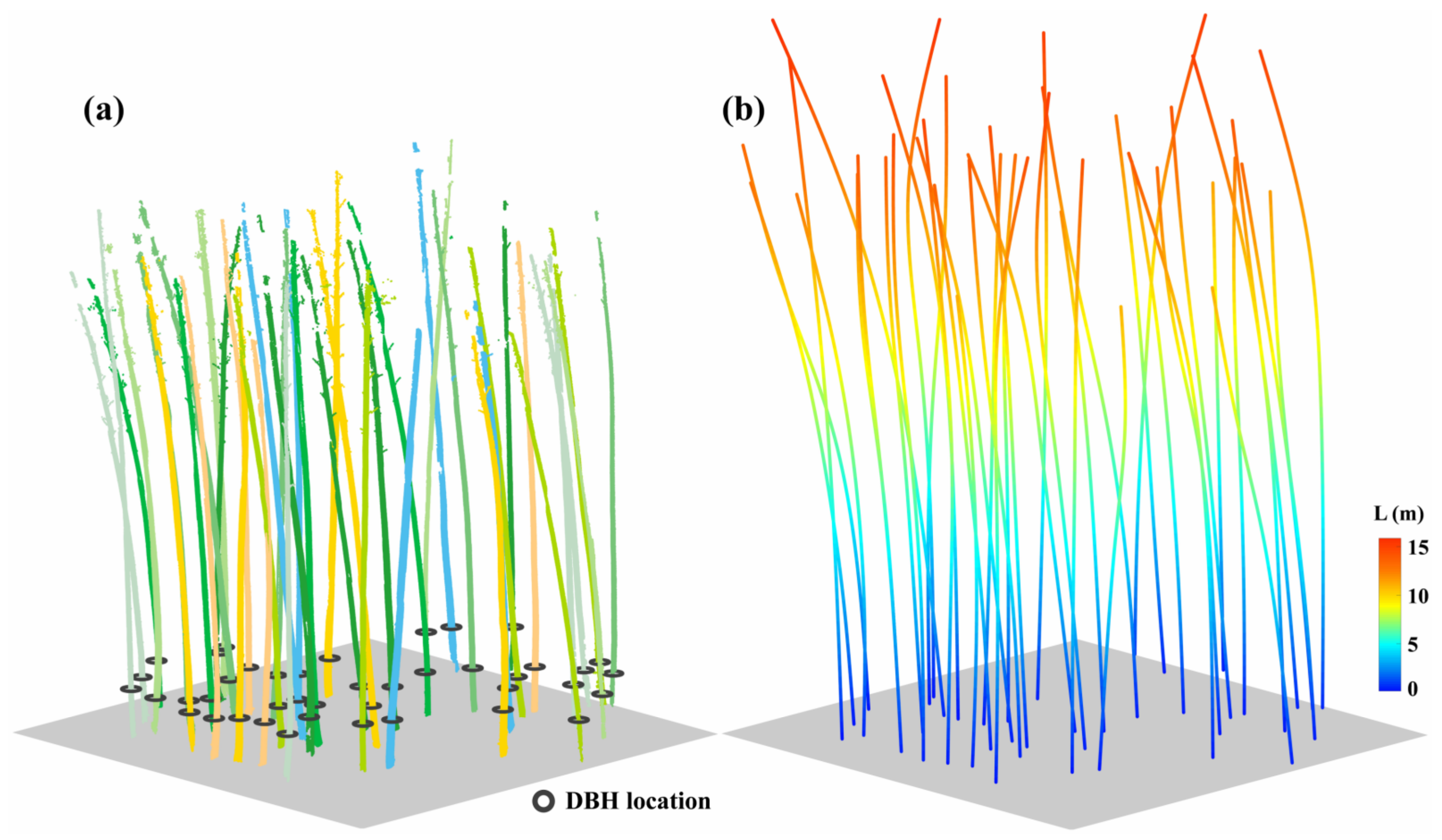
4.1. Segmented Individual Bamboos

As shown in Figure 7, there were 42 Moso bamboos segmented from the point cloud of the sample plot using the layer-wise distance discrimination method. The rate of correct detection was as high as 100% (Figure 7a). Among them, 38 bamboos were completely segmented, and the canopies of the remaining 4 bamboos were partially segmented (Figure 7b). Incomplete segmentation usually included two cases: over-segmentation and under-segmentation. Hence, the complete segmentation precision was 90.4%. Refer to Section 5.1 for the comparison with other segmentation algorithms.

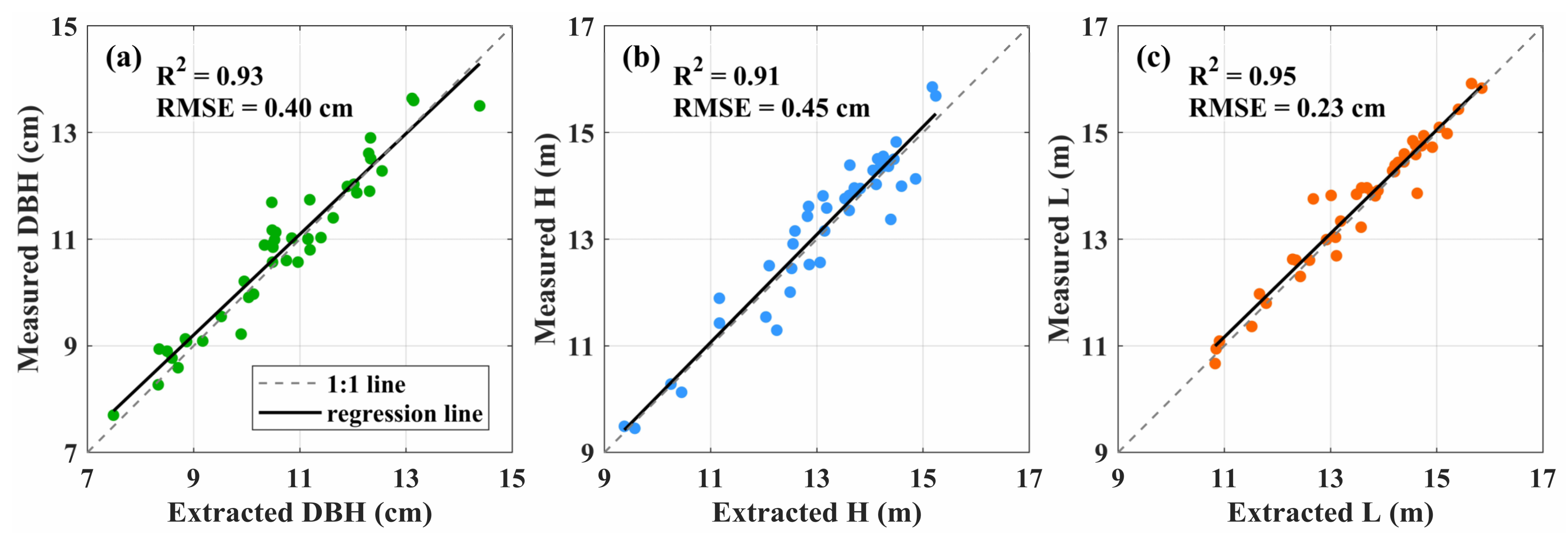
4.2. Extracted Structure Parameters

As indicated in Figure 8a, the DBHs were extracted by circle fitting from the segmented culm points of individual Moso bamboos. As statistics show in Table 2, the bamboo DBHs ranged from 7.49 cm to 14.39 cm, with a mean value of 10.69 cm. The R 2 and R M S E of the extracted DBHs were 0.93 cm and 0.40 cm (Figure 9a), indicating the effectiveness of the circle fitting method in automatically obtaining the individual DBHs from the point cloud scanned by TLS. According to Equation (15), the negative value of the AE meant underestimation, and the positive value implied overestimation. As the calculated A E s varied from −1.22 cm to 0.88 cm, the extracted DBHs exhibited slight misestimations. On one hand, the bamboo culms were possibly occluded by the adjacent low vegetation, and the point cloud scanned by the TLS were not enough for circle fitting. On the other hand, the cross-sections of the Moso bamboo culms might not be strictly round.
As for the normalized point cloud, the H of an individual Moso bamboo was actually the maximum height of its belonging points. The H and L of individual Moso bamboos were extracted, respectively, from the constructed bamboo culm axes (Figure 8b). As listed in Table 2, the extracted H ranged from 9.38 m to 15.24 m with a mean value of 13.14 m. The R 2 and R M S E of the extracted Hs of individual Moso bamboos against the corresponding measured Hs were 0.91 m and 0.45 m, respectively (Figure 9b). The A E s of extracted Hs varied from −0.77 m to 1.02 m, and the number of underestimated Hs exceeded that of overestimated ones. It might be because that the broken parts of the bamboo culm point cloud principally appeared near the bamboo tops.
As shown in Table 2, the extracted Ls ranged from 10.83 m to 15.85 m with a mean value of 13.58 m. According to Figure 9c, the R 2 and R M S E of the extracted Ls of individual Moso bamboos against the manually measured Ls were 0.95 m and 0.23 m, which indicated that there was a high correlation between the extracted and measured Ls. The calculated AEs ranged from –1.08 m to 0.77 m, demonstrating the effectiveness of constructing the bamboo culm axis from the point cloud and calculating their lengths in segments. The major error of extracted L first arose from the point cloud segmentation. The segmentation accuracy of an individual Moso bamboo directly affected the capture of the culm tip in the construction of the culm axis. Another error source was the presence of broken points in the culm points located in the canopy, which affected the extraction accuracy of the cross-section center points.

4.3. Estimated AGB

The AGBs of individual Moso bamboos in the study site were estimated based on their Hs and Ls using Equation (11) and Equation (12), respectively. According to the statistics in Table 3, the AGB H s ranged from 7.82 kg to 25.48 kg, with a mean value of 16.12 kg, and the AGB L s from 8.01 kg to 25.62 kg, with a mean value of 16.58 kg. The AGB H and AGB L of each Moso bamboo were shown in the same column in Figure 10a, and it could be seen that the AGB H was generally less than the corresponding AGB L . As indicated in Figure 10b, the difference between the individual AGB H and AGB L ranged from 0.06 kg to 2.33 kg, which was principally determined by the specific bending degree of the bamboo culm. Compared with the AGB L , the AGB H had an underestimation of about 0.46 kg per bamboo, which accounted for approximately 2.85% of the mean AGB H . As a result, the total AGBs of the Moso bamboos in the sample plot were estimated as 680.40 kg and 696.36 kg, based on H and L, respectively.

5. Discussion

5.1. Comparison of Individual Bamboo Segmentation Algorithms

The LDD method proposed in our study was compared with two popular methods for individual tree segmentation at the single bamboo level, including the comparative shortest-path algorithm (CSP, implemented in the LiDAR360 software) [22] and graph-pathing algorithm (GP, implemented in the lidUrb package) [14]. The CSP algorithm utilized a comparative shortest path to determine the belonging trees of the candidate points, which attained a high efficiency in individual tree segmentation. The key step of the GP algorithm was to walk through each node within the point cloud graph, and it was able to achieve an accurate segmentation of individual trees with large canopies.
According to the distance between bamboo culms and the interlacing degree of bamboo canopies, four typical scenes in a Moso bamboo forest were selected for assessing the performances of the three algorithms. Scene 1: bamboo locations were relatively independent; Scene 2: the distances between bamboo culms were relatively close; Scene 3: the bamboo canopies were seriously interlaced; Scene 4: the bamboo stand had a complex structure (a combination of Scenes 2 and 3). The segmentation results of CSP, GP, and LDD separately applied to the four scenes were shown in Figure 11a–c. Specifically, all three algorithms performed well in Scene 1 (Figure 11(a1–c1)). As for Scene 2 (Figure 11(a2–c2)), CSP did not correctly separate the bamboos; GP successfully separated the bamboo culms, but failed in the bamboo canopy segmentation; LDD correctly separated the bamboo points, including culms and canopies. In the limited space, Moso bamboos had to compete for a larger living space, resulting in serious overlapping and interlacing between bamboo canopies [5]. In this situation, it was very difficult to completely separate the individual bamboos. As shown in Figure 11(a3–c3,a4–c4), the three algorithms suffered from canopy under-segmentation or over-segmentation to various extents in Scenes 3 and 4. Especially, GP had segmented a single bamboo into two parts (Figure 11(b3)). The layer-wise clustering and the preset conditions for discriminating cross-section center points in LDD effectively conformed to the growth characteristics of the Moso bamboos, making it more robust to segment bent bamboos. In practice, however, as indicated in Figure 11(c4), a fraction of the canopy points of adjacent Moso bamboos were wrongly assigned to the target Moso bamboo due to the serious canopy occlusion. Comparatively, LDD demonstrated superior segmentation performances in various scenes of the Moso bamboo forest. According to inherent characteristics and advantages, LDD is generalizable in stands with irregular growth shapes and close spacing. However, LDD relies on accurate seed point identification and has some limitations for stands with relatively dense understory vegetation.

5.2. Comparison of Bamboo Culm Axis Construction Methods

After individual bamboo segmentation, there were two key steps to obtain the bamboo culm length. The first step was to extract the cross-section centers, and the second was to construct the culm axis from those extracted centers. As for extracting the cross-section centers, two possible methods were tested. One was to calculate the convex hull centroids of all point layers of a single bamboo (denoted as A1). The other was the combined method adopted in our study (A2). The cross-section centers of culm points were extracted using circle fitting, while those of the B&F points were obtained by calculating the convex hull centroids of the point layers. As for constructing bamboo culm axes, three potential methods were tried. The first was to directly connect the adjacent cross-section centers of a single bamboo using line segments and add their lengths as the bamboo L (denoted as B1). The second was the method that was described in Section 3.2 (B2). The five equally spaced cross-section centers were selected as the feature points, which were fitted with four cubic B-spline curve segments. The total bamboo length was obtained by summing the lengths of the four curve segments. The third was to take all cross-section centers as feature points and use cubic B-spline curve segments to fit and calculate the bamboo length (B3).
Therefore, there were six different combinations between the methods of extracting the cross-section centers, and constructing the culm axes. As indicated in Figure 12, the accuracies of the extracted bamboo lengths by various combinations were separately assessed. The best accuracy was achieved by the combination of A2-B2, with the highest R2 of 0.95 and the lowest RMSE of 0.23 m. This was the method combination adopted for the bamboo length extraction in our study. A2 showed higher performance only when combined with B2. However, the best performance of B2 was probably determined by the 3D spatial distribution characteristics of the extracted cross-section center points. All of the extracted culm centers of a single bamboo did not lie exactly on a smooth longitudinal axis, but were randomly distributed around it. If all cross-section center points were involved in the construction of the bamboo culm axis, the errors would be accumulated. Accordingly, the accuracies of the extracted culm lengths by the combinations, including B1 or B3, would be seriously reduced.

5.3. Error Sources and Potential Improvements

Although we used a TLS to achieve more an accurate AGB estimation in a Moso bamboo forest, there were still some factors that might affect the accuracy. For example, the four scanning stations were used to minimize B&F occluding, but the TLS scanning in the vertical direction was unavoidably blocked by the adjacent bamboo canopies [43], resulting in inadequate scanned points for the target bamboo canopy. Although generally achieving superior results in individual bamboo segmentation, the LDD inevitably segmented the canopy points to the wrong neighboring Moso bamboo in a stand of ultra-high density. In this situation, the proper manual adjustments became necessary. During the automatic estimation of the bamboo culm length, the fitted bamboo culm axis might introduce some errors due to the difficulty in accurately locating the bamboo tops. In addition, the AGB of the Moso bamboo in the study site might not be precisely estimated due to the direct adoption of the allometric equation and its coefficients provided in the literature.
Nevertheless, some measures can be taken to further improve the accuracy of Moso bamboo AGB estimation. For example, the point cloud of the bamboo canopy tops could be obtained using UAV-borne LiDAR, which can be fused with TLS-acquired point cloud to improve the extraction accuracy of the bamboo culm length [44]. In addition, the allometric equation can be determined by local experiments rather than directly using empirical models in the literature [45].

6. Conclusions

In this study, we proposed a workflow for the refined estimation of Moso bamboo AGB using culm lengths extracted from the point cloud data scanned by a TLS. The key steps included individual bamboo segmentation, extraction of structural parameters (DBH and L), and a refined estimation of individual bamboo AGB. The major conclusions we reached were as follows:
  • The layer-wise distance discrimination method demonstrated superior performance in segmenting the individual Moso bamboos in a dense stand. The rate of the correct detection of bamboo culms was as high as 100%, and the precision of the complete segmentation of individual bamboo points was 90.4%;
  • The bamboo culm axis was automatically constructed by extracting the center points of the culm cross-sections on a layer-by-layer base. The total culm length of a bent Moso bamboo was accurately obtained by summing the lengths of the four segments fitted by cubic B-spline curves, with the R 2 and R M S E of 0.95 m and 0.23 m;
  • The AGB H of an individual Moso bamboo was generally less than the corresponding AGB L . The difference was positively correlated with the bending degree of the bamboo culm. The total estimated AGB of the Moso bamboos in the study site increased by 2.85% from 680.40 kg on H to 696.36 kg on L.
Although our study achieved a refined estimation of Moso bamboo AGB, factors such as B&F shading, incomplete point cloud scanning, and ineffective segmentation still affected the accuracy. Therefore, the accurate estimation of Moso bamboo AGB in dense stands is still a very challenging task. In practice, the more suitable scanning design and segmentation method should be chosen to achieve a more accurate estimation of Moso bamboo AGB according to the actual situation of the study site. In addition, the fusion of the point clouds, acquired by TLS and UAV-borne LiDAR, is desirable to more accurately extract the culm lengths of Moso bamboos in a dense stand and could be a promising topic in future studies.

Author Contributions

Conceptualization, J.L.; methodology, J.L. and R.J.; validation, R.J.; formal analysis, J.L. and R.J.; investigation, J.L., R.J. and T.L.; data curation, T.L.; writing—original draft preparation, R.J.; writing—review and editing, J.L.; visualization, R.J.; supervision, J.L.; project administration, J.L.; funding acquisition, J.L. and R.J. All authors have read and agreed to the published version of the manuscript.

Funding

This research was funded by the National Natural Science Foundation of China, grant number 32071678; the Postgraduate Innovative Research Project of Chongqing, grant number CYS22204; and the Key Research and Development Program of the Sichuan Province, grant number 2022YFQ0035.

Data Availability Statement

Data available on request due to restrictions eg privacy or ethical.

Acknowledgments

The authors would like to thank Yangyu Chen from Southwest University, China for his help in field measuring and LiDAR point cloud acquiring.

Conflicts of Interest

The authors declare no conflict of interest. The funders had no role in the design of the study; in the collection, analyses, or interpretation of data; in the writing of the manuscript, or in the decision to publish the results.

References

  1. Xu, X.; Du, H.; Zhou, G.; Ge, H.; Shi, Y.; Zhou, Y.; Fan, W. Estimation of aboveground carbon stock of Moso bamboo (Phyllostachys heterocycla var. pubescens) forest with a Landsat Thematic Mapper image. Int. J. Remote Sens. 2011, 32, 1431–1448. [Google Scholar] [CrossRef]
  2. Yuen, J.Q.; Fung, T.; Ziegler, A.D. Carbon stocks in bamboo ecosystems worldwide: Estimates and uncertainties. For. Ecol. Manag. 2017, 393, 113–138. [Google Scholar] [CrossRef]
  3. FAO. State of the World’s Forests 2014: Enhancing the Socioeconomic Benefits from Forests; FAO: Roma, Italy, 2014. [Google Scholar]
  4. Xu, J.D. The 8th Forest resourcements inventory results and analysis in China. For. Econ. 2014, 3, 6–8. [Google Scholar]
  5. Cao, L.; Coops, N.C.; Sun, Y.; Ruan, H.; She, G. Estimating canopy structure and biomass in bamboo forests using airborne LiDAR data. ISPRS J. Photogramm. Remote Sens. 2019, 148, 114–129. [Google Scholar] [CrossRef]
  6. Brown, S.; Gillespie, A.J.; Lugo, A.E. Biomass estimation methods for tropical forests with applications to forest inventory data. For. Sci. 1989, 35, 881–902. [Google Scholar]
  7. Khan, I.A.; Khan, W.R.; Ali, A.; Nazre, M. Assessment of above-ground biomass in pakistan forest ecosystem’s carbon pool: A review. Forests 2021, 12, 586. [Google Scholar] [CrossRef]
  8. Shen, X.; Jiang, M.; Lu, X.; Liu, X.; Liu, B.; Zhang, J.; Wang, Z. Aboveground biomass and its spatial distribution pattern of herbaceous marsh vegetation in China. Sci. China Earth Sci. 2021, 64, 1115–1125. [Google Scholar] [CrossRef]
  9. Wai, P.; Su, H.; Li, M. Estimating Aboveground Biomass of Two Different Forest Types in Myanmar from Sentinel-2 Data with Machine Learning and Geostatistical Algorithms. Remote Sens. 2022, 14, 2146. [Google Scholar] [CrossRef]
  10. Gibbs, H.K.; Brown, S.; Niles, J.O.; Foley, J.A. Monitoring and estimating tropical forest carbon stocks: Making REDD a reality. Environ. Res. Lett. 2007, 2, 045023. [Google Scholar] [CrossRef] [Green Version]
  11. Wehr, A.; Lohr, U. Airborne laser scanning—An introduction and overview. ISPRS J. Photogramm. Remote Sens. 1999, 54, 68–82. [Google Scholar] [CrossRef]
  12. Dassot, M.; Constant, T.; Fournier, M. The use of terrestrial LiDAR technology in forest science: Application fields, benefits and challenges. Ann. For. Sci. 2011, 68, 959–974. [Google Scholar] [CrossRef] [Green Version]
  13. Zheng, G.; Moskal, L.M.; Kim, S.H. Retrieval of effective leaf area index in heterogeneous forests with terrestrial laser scanning. IEEE Trans. Geosci. Remote Sens. 2012, 51, 777–786. [Google Scholar] [CrossRef]
  14. Wang, D.; Liang, X.; Mofack, G.I.; Martin-Ducup, O. Individual tree extraction from terrestrial laser scanning data via graph pathing. For. Ecosyst. 2021, 8, 67. [Google Scholar] [CrossRef]
  15. Feldpausch, T.R.; Lloyd, J.; Lewis, S.L.; Brienen, R.J.; Gloor, M.; Monteagudo Mendoza, A.; Lopez-Gonzalez, G.; Banin, L.; Abu Salim, K.; Affum-Baffoe, K. Tree height integrated into pantropical forest biomass estimates. Biogeosciences 2012, 9, 3381–3403. [Google Scholar] [CrossRef] [Green Version]
  16. Silva, C.A.; Hudak, A.T.; Vierling, L.A.; Loudermilk, E.L.; O’Brien, J.J.; Hiers, J.K. Imputation of individual longleaf pine (Pinus palustris Mill.) tree attributes from field and LiDAR data. Can. J. Remote Sens. 2016, 42, 554–573. [Google Scholar] [CrossRef]
  17. Cabo, C.; Ordóñez, C.; López-Sánchez, C.A.; Armesto, J. Automatic dendrometry: Tree detection, tree height and diameter estimation using terrestrial laser scanning. Int. J. Appl. Earth Obs. Geoinf. 2018, 69, 164–174. [Google Scholar] [CrossRef]
  18. Simonse, M.; Aschoff, T.; Spiecker, H.; Thies, M. Automatic Determination of Forest Inventory Parameters Using Terrestrial Laserscanning. In Proceedings of the ScandLaser Scientific Workshop on Airborne Laser Scanning of Forests, Umeå, Sweden, 3–4 September 2003; pp. 251–257. [Google Scholar]
  19. Edson, C.; Wing, M.G. Airborne light detection and ranging (LiDAR) for individual tree stem location, height, and biomass measurements. Remote Sens. 2011, 3, 2494–2528. [Google Scholar] [CrossRef] [Green Version]
  20. Li, W.; Guo, Q.; Jakubowski, M.K.; Kelly, M. A new method for segmenting individual trees from the lidar point cloud. Photogramm. Eng. Remote Sens. 2012, 78, 75–84. [Google Scholar]
  21. Maas, H.G.; Bienert, A.; Scheller, S.; Keane, E. Automatic forest inventory parameter determination from terrestrial laser scanner data. Int. J. Remote Sens. 2008, 29, 1579–1593. [Google Scholar] [CrossRef]
  22. Tao, S.; Wu, F.; Guo, Q.; Wang, Y.; Li, W.; Xue, B.; Hu, X.; Li, P.; Tian, D.; Li, C. Segmenting tree crowns from terrestrial and mobile LiDAR data by exploring ecological theories. ISPRS J. Photogramm. Remote Sens. 2015, 110, 66–76. [Google Scholar] [CrossRef] [Green Version]
  23. Xing, W.L.; Xing, Y.Q.; Huang, Y.; Qu, L.; You, H.T. Individual tree segmentation of TLS point cloud data based on clustering of voxels layer by layer. J. Cent. S. Univ. Forest. Technol. 2017, 37, 58–6471. [Google Scholar]
  24. Su, Z.; Li, S.; Liu, H.; Liu, Y. Extracting wood point cloud of individual trees based on geometric features. IEEE Geosci. Remote Sens. Lett. 2019, 16, 1294–1298. [Google Scholar] [CrossRef]
  25. Wang, J.; Chen, X.; Cao, L.; An, F.; Chen, B.; Xue, L.; Yun, T. Individual rubber tree segmentation based on ground-based LiDAR data and faster R-CNN of deep learning. Forests 2019, 10, 793. [Google Scholar] [CrossRef] [Green Version]
  26. Zhang, R.; Zhou, X.; Ouyang, Z.; Avitabile, V.; Qi, J.; Chen, J.; Giannico, V. Estimating aboveground biomass in subtropical forests of China by integrating multisource remote sensing and ground data. Remote Sens. Environ. 2019, 232, 111341. [Google Scholar] [CrossRef]
  27. Lin, J.; Wang, M.; Ma, M.; Lin, Y. Aboveground tree biomass estimation of sparse subalpine coniferous forest with UAV oblique photography. Remote Sens. 2018, 10, 1849. [Google Scholar] [CrossRef] [Green Version]
  28. Bazezew, M.N.; Hussin, Y.A.; Kloosterman, E. Integrating Airborne LiDAR and Terrestrial Laser Scanner forest parameters for accurate above-ground biomass/carbon estimation in Ayer Hitam tropical forest, Malaysia. Int. J. Appl. Earth Obs. Geoinf. 2018, 73, 638–652. [Google Scholar] [CrossRef]
  29. Garms, C.G.; Strimbu, B.M. Impact of stem lean on estimation of Douglas-fir (Pseudotsuga menziesii) diameter and volume using mobile lidar scans. Can. J. For. Res. 2021, 51, 1117–1130. [Google Scholar] [CrossRef]
  30. Vitter, J.S. Faster methods for random sampling. Commun. ACM 1984, 27, 703–718. [Google Scholar] [CrossRef] [Green Version]
  31. Rusu, R.B.; Marton, Z.C.; Blodow, N.; Dolha, M.; Beetz, M. Towards 3D point cloud based object maps for household environments. Robot. Auton. Syst. 2008, 56, 927–941. [Google Scholar] [CrossRef]
  32. Zhang, W.; Qi, J.; Wan, P.; Wang, H.; Xie, D.; Wang, X.; Yan, G. An Easy-to-Use Airborne LiDAR Data Filtering Method Based on Cloth Simulation. Remote Sens. 2016, 8, 501. [Google Scholar] [CrossRef]
  33. Wang, D.; Hollaus, M.; Pfeifer, N. Feasibility of machine learning methods for separating wood and leaf points from terrestrial laser scanning data. ISPRS Ann. Photogramm. Remote Sens. Spatial Inf. Sci. 2017, 4, 157–164. [Google Scholar] [CrossRef] [Green Version]
  34. Liang, X.; Litkey, P.; Hyyppa, J.; Kaartinen, H.; Vastaranta, M.; Holopainen, M. Automatic stem mapping using single-scan terrestrial laser scanning. IEEE Trans. Geosci. Remote Sens. 2011, 50, 661–670. [Google Scholar] [CrossRef]
  35. Barber, C.B.; Dobkin, D.P.; Huhdanpaa, H. The quickhull algorithm for convex hulls. ACM Trans. Math. Softw. 1996, 22, 469–483. [Google Scholar] [CrossRef] [Green Version]
  36. Fischler, M.A.; Bolles, R.C. Random sample consensus: A paradigm for model fitting with applications to image analysis and automated cartography. Commun. ACM 1981, 24, 381–395. [Google Scholar] [CrossRef]
  37. West, P.W. Tree and Forest Measurement; Springer: Berlin/Heidelberg, Germany, 2003; pp. 39–44. [Google Scholar]
  38. Hou, H.; Andrews, H. Cubic splines for image interpolation and digital filtering. IEEE Trans. Acoust. Speech Signal Process. 1978, 26, 508–517. [Google Scholar]
  39. Liu, M.; Huang, Y.; Yin, L. Development and implementation of a NURBS interpolator with smooth feedrate scheduling for CNC machine tools. Int. J. Mach. Tools Manuf. 2014, 87, 1–15. [Google Scholar] [CrossRef]
  40. You, L.; Ha, D.L.; Xie, M.K.; Zhang, X.P.; Song, X.Y.; Pang, Y.; Tang, S.Z. Stem Volume Calculation Based on Stem Section Profile Curve and Three Dimension Laser Point Cloud. Sci. Silvae Sin. 2019, 55, 63–72. [Google Scholar]
  41. Ni, X.W.; Huang, X.; Zhu, R. A Highly-efficient Pose Synchronization Planning Method for Industrial Robot Free-form Curve Motion. Mach. Tool Hydraul. 2021, 49, 34–39, 59. [Google Scholar]
  42. Zheng, J.X.; Dong, W.Y. A Study on Over ground Biomass Structure of Clone Population of Natural Phyllostachys pubescens in Haiziping. For. Inventory Plan. 2009, 34, 30–33. [Google Scholar]
  43. Beyene, S.M. Estimation of Forest Variable and Aboveground Biomass using Terrestrial Laser Scanning in the Tropical Rainforest. J. Indian Soc. Remote Sens. 2020, 48, 853–863. [Google Scholar] [CrossRef]
  44. Shimizu, K.; Nishizono, T.; Kitahara, F.; Fukumoto, K.; Saito, H. Integrating terrestrial laser scanning and unmanned aerial vehicle photogrammetry to estimate individual tree attributes in managed coniferous forests in Japan. Int. J. Appl. Earth Obs. Geoinf. 2022, 106, 102658. [Google Scholar] [CrossRef]
  45. Lin, J.; Chen, D.; Wu, W.; Liao, X. Estimating aboveground biomass of urban forest trees with dual-source UAV acquired point clouds. Urban For. Urban Green. 2022, 69, 127521. [Google Scholar] [CrossRef]
Figure 1. (a) The location of Hutou Village; (b) top view of the study site; (c) point cloud of sample plot after preprocessing.
Remotesensing 14 05537 g001
Figure 2. Process diagram of point cloud preprocessing: (a) registration of multiple station point clouds; (b) point cropping, thinning, and outlier removing; (c) separation of bamboo and ground points; (d) height normalization of bamboo points.
Remotesensing 14 05537 g002
Figure 3. Process of generating seed points: (a) selected horizontal strip; (b) identified positions of individual Moso bamboos; (c) generated seed points at the culm height of 1.3 m.
Remotesensing 14 05537 g003
Figure 4. Schematic diagram of layer-wise distance discrimination segmentation: (a) the clustering centers of layers of individual Moso bamboos; (b) point clustering in a layer of canopy points; (c) point clustering in a layer of culm points.
Remotesensing 14 05537 g004
Figure 5. Process of the bamboo point separation: (a) horizontal layering of bamboo points; (b) detect straight line using RANSAC; (c) separated bamboo culm points; (d) separated bamboo B&F points.
Remotesensing 14 05537 g005
Figure 6. Process of bamboo culm axis construction: (a) The point cloud used to extract the cross-section center points; (b) extraction of the centroid of point cloud using convex hull; (c) extraction of circle center using RANSAC; (d) construction of bamboo culm axis using cubic B-spline curves.
Remotesensing 14 05537 g006
Figure 7. (a) Measured and detected locations of individual Moso bamboos; (b) segmented points of individual Moso bamboos.
Remotesensing 14 05537 g007
Figure 8. (a) Segmented culm points and extracted DBHs of individual Moso bamboos; (b) constructed bamboo culm axes using cubic B-spline curves.
Remotesensing 14 05537 g008
Figure 9. Accuracy assessment of extracted structural parameters of individual Moso bamboos: (a) DBH; (b) H; (c) L.
Remotesensing 14 05537 g009
Figure 10. (a) AGB H s and AGB L s of individual Moso bamboos; (b) Differences between individual AGB H s and AGB L s.
Remotesensing 14 05537 g010
Figure 11. Segmentation results in the four typical scenes of Moso bamboos: (a) CSP; (b) GP; (c) LDD.
Remotesensing 14 05537 g011
Figure 12. Accuracy assessment of extracted bamboo lengths by different method combinations of extracting cross-section centers and constructing culm axes.
Remotesensing 14 05537 g012
Table 1. Statistics of the measured DBHs, Hs, and Ls of individual Moso bamboos.
ParametersNo.MinMaxMean
Measured DBH (cm)427.7013.6410.79
Measured H (m)429.4515.8513.23
Measured L (m)4210.6715.9213.67
Table 2. Statistics of the extracted DBHs, Hs, and Ls of individual Moso bamboos.
ParametersNo.MinMaxMean
Extracted DBH (cm)427.4914.3910.69
Extracted H (m)429.3815.2413.14
Extracted L (m)4210.8315.8513.58
Table 3. Statistics of the estimated AGBs of individual Moso bamboos based on H and L, respectively.
AGBNo.MinMaxMean
AGB H (kg)427.82 25.48 16.12
AGB L (kg)428.01 25.62 16.58
Publisher’s Note: MDPI stays neutral with regard to jurisdictional claims in published maps and institutional affiliations.

