Embedded Feature Selection and Machine Learning Methods for Flash Flood Susceptibility-Mapping in the Mainstream Songhua River Basin, China

Abstract

Mapping flash flood susceptibility is effective for mitigating the negative impacts of flash floods. However, a variety of conditioning factors have been used to generate susceptibility maps in various studies. In this study, we proposed combining logistic regression (LR) and random forest (RF) models with embedded feature selection (EFS) to filter specific feature sets for the two models and map flash flood susceptibility in the mainstream basin of the Songhua River. According to the EFS results, the optimized feature sets included 32 and 28 features for the LR and RF models, respectively, and the composition of the two optimal feature sets was similar and distinct. Overall, the relevant vegetation cover and river features exhibit relatively high effects overall for flash floods in the study area. The LR and RF models provided accurate and reliable flash flood susceptibility maps (FFSMs). The RF model (accuracy = 0.8834, area under the curve (AUC) = 0.9486) provided a better prediction capacity than the LR model (accuracy = 0.8634, AUC = 0.9277). Flash flood-prone areas are mainly distributed in the south and southwest and areas close to rivers. The results obtained in this study is useful for flash flood prevention and control projects.

1. Introduction

Floods are one of the most frequent natural disasters on Earth [1]. In recent years, flood risk has increased with global climate change [2,3]. Flash floods, characterized by the rapid formation of flood conditions, often result in severe life and property losses due to their strong suddenness and high flow rates [4,5]. Flash floods are the active exhibitions of surface runoff on slopes and are caused by heavy rainfall that lasts only a few hours [6]. Rapid flash flood outbreaks pose a challenge for risk management in basins and make timely communication and decision-making difficult [7]. Therefore, the key subjects related to the assessment and warning of flash floods have been widely studied by the research community at various catchment and regional scales [8].

Flash flood susceptibility maps (FFSMs) play an essential role in risk mitigation and are considered effective tools for alleviating the harmful effects and risks associated with flash floods [9]. An FFSM generally defines areas in which the likelihood of a flash flood occurring ranges from very low to very high; this likelihood is related to the physical and geographical characteristics of the corresponding areas [6,10]. This method can be used over large areas, such as entire river basins, because it provides useful guidance for decision-makers to effectively manage locations that are at risk of flash flood disasters [1]. Hence, it is essential to produce reliable and accurate FFSMs for flash flood-prone basins. FFSMs are spatially predicted using the assumption that future floods could occur under circumstances similar to those that caused previous flash floods [9]. In recent years, the hazard susceptibility assessment methods applied over large areas globally have mainly focused on the use of machine learning algorithms, such as logistic regression (LR) [11,12], frequency ratios [13,14], decision trees [15,16], support vector machines [14,17], random forests (RFs) [12,18], and artificial neural networks [10,12]. Promising results have been achieved using these methods by inputting many conditioning factors. However, models are paid more attentions by studies, with little attention to how the factors inputted into the model are selected.

Conditioning factor datasets containing different numbers and compositions of factors have been selected and applied to map flash flood susceptibility in multiple studies, namely, nine factors were used for developing FFSM in the northwest mountainous region of Vietnam [19], and fifteen factors were selected as independent variables for flash flood susceptibility modeling in Iran [9]. In China, twelve geographic, meteorological, and hydrological explanatory factors were selected for mapping flood susceptibility on a national scale [20], and eleven flood related variables were used for construction of a flood susceptibility map in Poyang County [21]. Generally, these conditioning factors are chosen based on the results of previous studies, expert knowledge, and the availability of data. There are currently no criteria for selecting conditioning factors for susceptibility mapping. However, previous studies have suggested that it is important to choose an effective set of conditioning factors in the process of modeling flash flood susceptibility [22]. Factors that are uncorrelated with flash flood phenomena, i.e., factors with very low predictive capabilities, may generate noisy input data, which may result in the applied models having decreased predictive capabilities [6]. In general, all candidate conditioning factors have certain predictive capabilities for flash flood modeling. However, selecting the most relevant conditioning factors may be suboptimal when building a predictor, especially if some factors are redundant. In contrast, the selection of a subset of useful features may remove many relevant but redundant features [23]. Various machine learning models have specific feature-learning characteristics, and the choice of a proper feature selection method can maximize the classification ability of these models [1]. Therefore, the present paper focuses on constructing and selecting feature subsets that are useful for constructing high-accuracy susceptibility maps.

Feature selection techniques can assist in removing irrelevant variables with low predictive power [24], and these techniques can be roughly grouped into three main categories, namely filter, wrapper, and embedded methods [25]. Filter methods preprocess features to remove the features that are unlikely to be useful for the model without considering the employed model [26]. For instance, the predictive ability of the factors was assessed for selection using information gain ratio [6,22]; correlation-based feature selection was filtered by finding relevant factors [27]. The disadvantages of filtering methods are that they ignore the interaction with the classifier and each feature is considered separately, thus ignoring feature dependencies [28]. Wrapper methods use the predictor as a black box to test each subset of potential features and select the subset that maximizes performance [29]. Generally, widely-used wrapper-based feature selection methods include genetic algorithms [24] and sequential forward selection [30]. However, this kind of method has a higher risk of overfitting and is very computationally intensive, requiring a considerable training time [28,31]. Furthermore, the order in which subsets are input in wrapper methods directly impacts the feature selection results [32,33]. Compared to the two types of methods described above, embedded methods incorporate feature selection as part of the model-training process and can select features that are most suitable for a certain model [23,34]. Embedded methods have the advantage of including interaction with the classification model while being significantly less computationally intensive than wrapper methods [28]. Consequently, we select machine learning algorithms that allow the use of embedded feature selection (EFS), namely, LR and RF models, to analyze and map flash flood susceptibility in this study.

China is among the countries plagued by flash floods, which seriously threaten the safety of people’s lives and property [35]. The Songhua River Basin is the main flood-affected area and an important river basin in Northeast China. In this context, the main purpose of the present study is to employ two classical machine learning algorithms, namely, LR and RF, in combination with an EFS method to assess flash flood susceptibility in the mainstream basin of the Songhua River. We compare the results obtained from the two algorithms in terms of (1) the identification of features that considerably influence the flash flood occurrence in the study area following the use of EFS and (2) the ability of the models to simulate flash flood susceptibility. The predictive results of the models and the importance of the selected features are discussed, with a particular focus on their commonalities and differences between the two models. FFSMs of the study area are also generated using each method considering the selected variables.

2. Study Area

The study area is the mainstream basin of the Songhua River in Northeast China; this region spans Jilin and Heilongjiang Provinces (Figure 1). It lies between 124°39′E and 132°31′E and between 43°01′N and 48°39′N, with a total area of approximately 1.93 × 105 km². The orographic conditions manifest in a clear contrast between mountainous areas and plains. Approximately 45% of the land surface is mountainous, and the highest peak reaches an elevation of 1694 m. The Mudan, Lalin, and Hulan Rivers are the dominant tributaries of the Songhua River in this region. The study area has a continental monsoon climate in a middle temperate zone, with cold winters and hot summers. The mean annual precipitation is approximately 526.8 mm. However, the precipitation distribution is uneven throughout the seasons due to monsoon conditions. Almost 70% of the annual precipitation falls from June to September; this period is regarded as the flood season in the study area. Moreover, this area is sensitive to intense rainfall making it difficult to provide warning in advance for flash flood protection. Flash flood mitigation in the mainstream basin of the Songhua River is a key component of emergency management. Hence, the accurate identification of flash flood-prone areas in this region has been highlighted by the government and discussed in the “Songhua River Basin Comprehensive Plan (2012–2030)” [36].

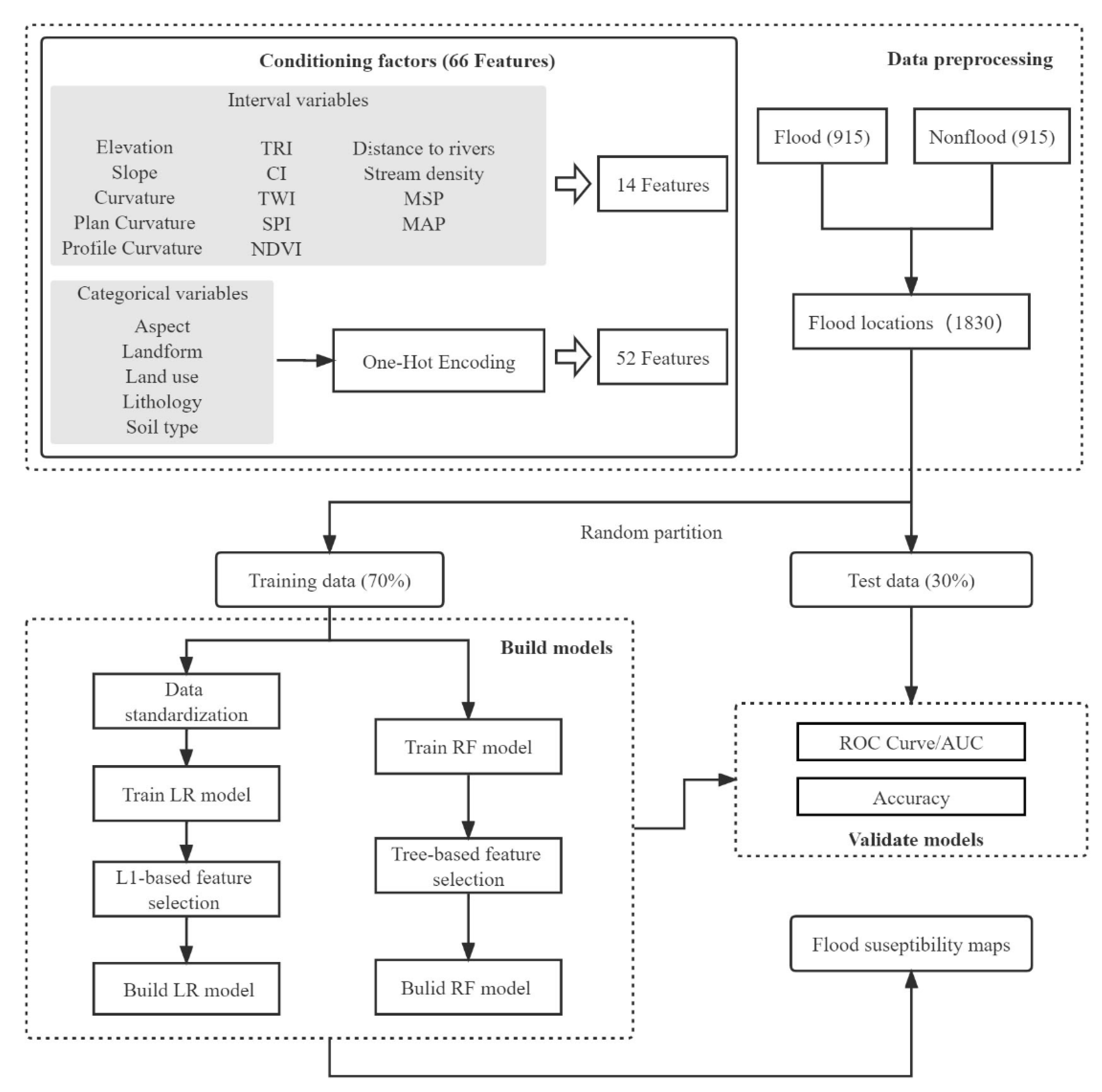
3. Data Preparation

3.1. Flash Flood Inventory

The basic idea of susceptibility modeling is that the factors that caused flash floods in the past will affect the likelihood of flash floods in the future [19]. Therefore, historical flash flood records are very important for susceptibility mapping. There are 915 events in the study area, which were extracted from the digital inventory of Chinese flash flood [37] (Figure 1). This dataset was generated by historical records and field surveys.

3.2. Flash Flood Conditioning Factors

According to published lectures, a number of conditioning factors have been employed to model the spatial patterns of flash flooding [5,9,16,35,38]. Various conditioning factors have been selected to map flash flood susceptibility in different regions. Some conditioning factors may contribute to the occurrence of flash floods in a particular area; however, the same factors may have less effect on flash floods in other regions [39]. Thus, the occurrence regime of flash floods is very complicated. In the present study, 19 potential conditioning factors were selected based on expert opinions, previous studies and the availability of data. These conditioning factors included the elevation [14], slope [40], aspect [13], curvature [41], plan curvature [21], profile curvature [21], landform, terrain ruggedness index (TRI) [42], convergence index (CI) [43], topographic wetness index (TWI) [44], stream power index (SPI) [14], distance to rivers [17], stream density [45], land use [13], normalized difference vegetation index (NDVI) [5], lithology [46], soil type [15], mean summer precipitation (MSP), and mean annual precipitation (MAP) [47].

The elevation, slope, aspect, curvature, plan curvature, profile curvature, CI, TRI, SPI, and TWI information were extracted from the Shuttle Radar Topography Mission (STRM) digital elevation model (DEM) product at a 90-m resolution (Figure 2). Because water flows from high elevations to low elevations, low-elevation areas are prone to flash floods [14,40]. The slope directly influences surface runoff fluidity and vertical seepage. Aspect is defined as the direction of the maximum slope of the topographic surface faces; this factor affects both the soil moisture content and local climatic conditions [13]. The curvature of an area reflects the concavity of the ground surface and affects flooding in a given area [41], and the plan curvature is perpendicular to the direction of the maximum slope and is related to the convergence and divergence of water flows across the land surface [21]. The profile curvature is parallel to the direction of the maximum slope and affects the acceleration or deceleration of water flowing across the land surface [21]. The CI gives a measure of how the water flowing in a cell diverges (CI < 0) or converges (CI > 0). The TRI is calculated as the sum of the elevation changes between a grid cell and its eight neighboring grid cells and can be used to objectively and quantitatively measure the topographic heterogeneity in the study region [42]. The TWI describes the humidity of the studied terrain and reveals spatial variations in the wetness of a basin. The SPI is related to erosion processes and is an indicator of the capability of flowing water to generate net erosion. The TWI and SPI are defined by the following equations:

$$\mathrm{TWI}=ln\left(A_s/tan\beta \right)$$

(1)

$$\mathrm{SPI}=A_s tan\beta$$

(2)

where A_S represents the specific catchment area and β (radians) is the slope gradient [48].

A river represents the main discharge route for a flood. The distance from rivers and the stream density of the basin play a major role in the distribution and magnitude of flash floods [17,45]. Linear river data were obtained from the National Geomatics Center of China and used to calculate the stream density and distance to rivers data (Figure 3a,b). Land use controls the amount of infiltration and surface runoff and critically influences the runoff speed, interception, infiltration, and evapotranspiration associated with flash floods (Figure 3c) [13]. The GlobeLand30 dataset with a resolution of 30 m was used in this study. The NDVI is an important indicator of vegetation coverage. Areas with high vegetation and high forest densities have reduced surface runoff. The NDVI can be calculated using Equation (3):

$$\mathrm{NDVI}=\frac{R_{NIR}-R_R}{R_{NIR}+R_R}$$

(3)

where R_NIR is the reflectance in the infrared portion of the electromagnetic spectrum and R_R is the reflectance in the red portion. Based on the SPOT/VEGETATION NDVI dataset, an annual NDVI dataset since 1998 was generated by maximum value composition. Then, the NDVI values were obtained by taking the mean values of multiyear data (Figure 3d). Different lithological units have different sensitivities to floods [46]. The lithology and soil in an area control the occurrence of flooding in the corresponding watershed by controlling runoff and infiltration [16]. The lithologic classification of the study area was extracted from a 1:2.5 million geological map of the People’s Republic of China (Figure 3e). Moreover, a soil type map with 28 categories was extracted from the national soil type distribution map at the scale of 1:4 million (Figure 3f and Figure S1) [49]. The landform refers to the variations in terrain, and the data were obtained from “The Atlas of Geomorphology of the People’s Republic of China” (Figure 3g). Precipitation is considered an essential factor because flash floods are often triggered by high-intensity and short-term heavy rainfall. In our study, two precipitation factors, MAP and MSP, were selected according to the precipitation characteristics in the study area (Figure 3h,i). The precipitation data were derived from annual and monthly datasets of land surface data collected in China.

4. Methods

In this study, two popular machine learning algorithms, LR and RF, were employed to evaluate the spatial flash flood susceptibility pattern in the study area. Moreover, two embedded approaches were tested for feature selection. L1 and tree-based methods were used for feature selection with the LR and RF models, respectively. A flowchart of the methodology adopted in this study is shown in Figure 4, and the methodology consists of the following steps: i. data preprocessing, ii. building predictive flash flood susceptibility models, and iii. validating and comparing the constructed models.

The main content of the data-preprocessing step involves preparing a conditioning factor database and constructing a flash flood inventory map. There are no essential criteria for the resolution of susceptibility mapping. We followed common practice by transforming all factors to 90 × 90 m resolution which was up to DEM resolution [50]. Some of the conditioning factors selected herein are categorical variables, such as the aspect, landform, land use, lithology, and soil type. These variables are discrete and disordered and thus not suitable for machine learning algorithms. Therefore, we used one-hot encoding to process categorical features. One-hot encoding creates one binary attribute per variable category, with the attribute being equal to 1 when belonging to the category and equal to 0 otherwise. In the current study, the five categorical variables were converted to 52 features through one-hot encoding. Thus, the resulting conditioning factor database contained 66 features. Moreover, 915 non-flood points were randomly generated in the study area and combined with the flash flood data to construct the flash flood inventory map. Finally, the flash flood inventory map was randomly divided into two datasets, namely, training (70%) and test (30%) datasets.

4.1. Machine Learning Algorithms

The present study was performed to produce FFSMs of the mainstream basin of the Songhua River using LR and RF models. The proposed methods were implemented with the scikit-learn package based on the Python language environment. The package is an efficient and open-source data-mining and analysis tool [51].

4.1.1. Logistic Regression (LR)

LR is a popular multivariate statistical model used to obtain spatial predictions of various natural hazards; this model is capable of exploring the relationships between a binary response variable coded as 0/1 and an array of explanatory variables [12,43,52]. In flash flood susceptibility mapping, LR is used to identify statistical relationships between flash flood events (dependent variable) and conditioning factors (independent variables) based on the presence or absence of flash floods. The basic form of LR, which uses a logistic function to model a binary dependent variable, can be expressed with the following equation:

$$p=\frac{1}{1+e^{-z}}$$

(4)

where p is the flash flood occurrence probability at a particular pixel and ranges from 0 to 1. z is a value that ranges from −∞ to + ∞. The term z is defined by the following equation:

$$z={\theta }_0+{\theta }_1{x}_1+{\theta }_2{x}_2+\cdots +{\theta }_n{x}_n$$

(5)

where θ₀ is the intercept of the model, n is the number of independent variables, θ₁, θ₂, …, θ_n are the regression coefficients of each independent variable, and x₁, x₂, …, x_n are the independent variables.

4.1.2. Random Forest (RF)

The RF method is a powerful and flexible ensemble-learning approach that was systematically proposed by Breiman [53]. This method can be applied for classification, regression and unsupervised learning based on decision trees [18,54]. Each individual decision tree in the ensemble is built using bootstrap sampling based on the original training dataset. Furthermore, when each node is split during the construction of a tree, the best split is obtained from a randomly selected subset of input features. The final flash flood probability is determined by obtaining the average prediction output by all decision trees using the scikit-learn package. Moreover, two main hyperparameters must be defined: the number of decision trees in the forest and the maximum depth of each tree; these parameters are referred to as n_estimators and max_depth, respectively.

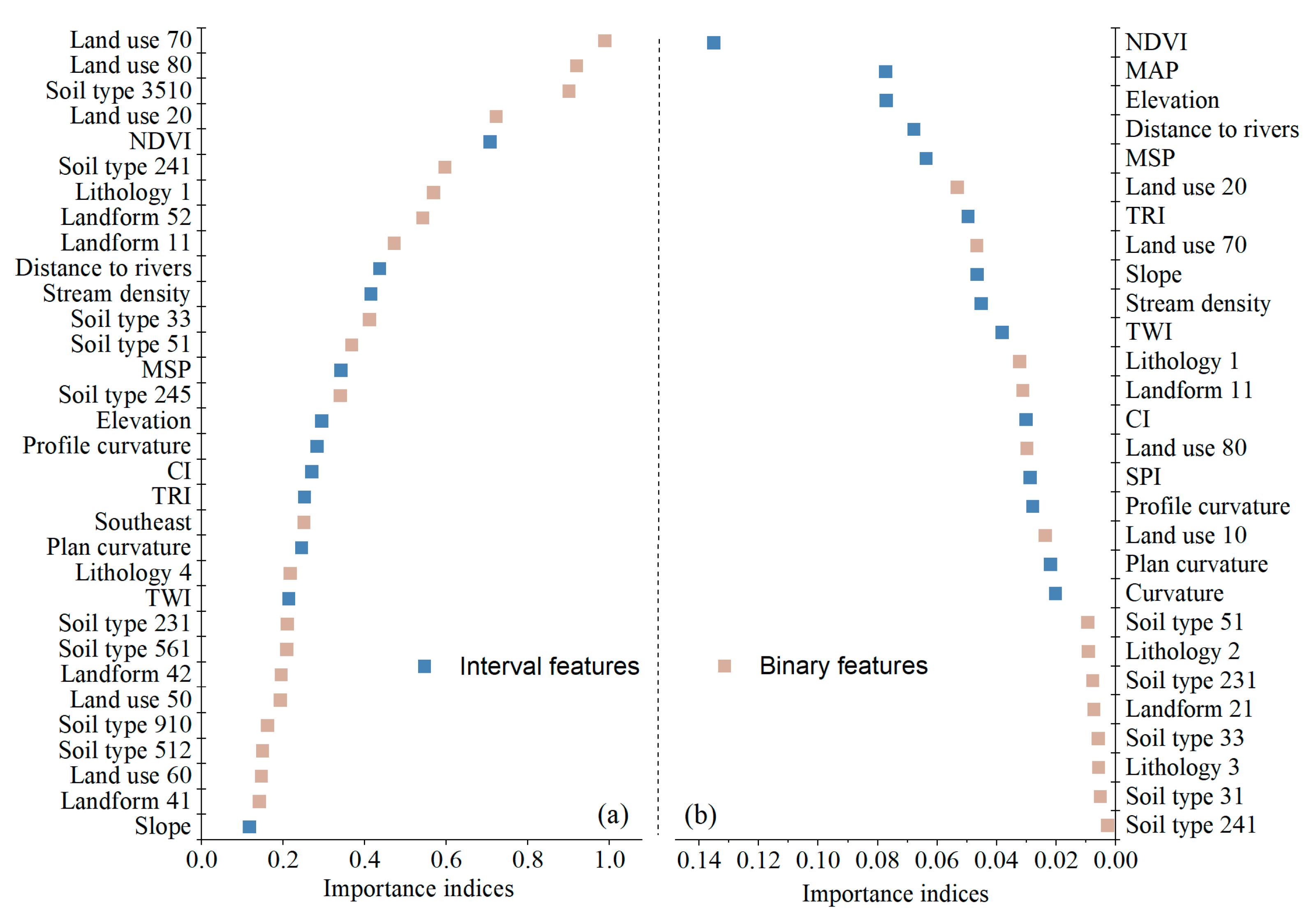
4.2. Embedded Feature Selection (EFS)

In this study, the feature selection approach is primarily used to remove noninformative or redundant features for constructing FFSMs. There are three general feature selection algorithms: filter, wrapper and embedded methods. Embedded methods are more efficient than wrapper methods and more accurate than filtering methods; in embedded methods, feature selection is performed during the training process. The most common types of EFS method are regularization and tree methods.

4.2.1. L1-Based Feature Selection for LR

Regularization is a common method used in machine learning. This method can limit the complexity of a model and prevent the occurrence of overfitting problems. In the current study, L1 regularization terms were introduced into the loss function of LR to implement EFS. The corresponding mathematical expression is as follows:

$${J\left(\theta \right)}_{\mathrm{L}1}=C\ast J\left(\theta \right)+\Vert \theta {\Vert }_1$$

(6)

where C is the hyperparameter used to control the degree of regularization, J(θ) is the loss function of LR, and ‖θ‖₁ is the L1 norm, namely, the penalty term. The L1 norm can be expressed as follows:

$$\Vert \theta {\Vert }_1={\displaystyle \sum }_{j=1}^n\left|{\theta }_j\right| \left(j\ge 1\right)$$

(7)

where n is the total number of features in the equation and θ_j represents each regression coefficient. The term j must have a value ≥1 because θ₀, the intercept, is not involved in regularization. The L1 regularization term can be used to effectively reduce the coefficients of some features to zero to allow features to be screened. The stronger the L1 regularization is, the fewer the number of features that are selected. In other words, the learning method based on L1 regularization is an EFS method. In this study, LR is used to filter the input features based on L1 regularization and to predict the occurrence of flash floods.

4.2.2. Tree-Based Feature Selection for RF

Feature selection is an inherent function of decision trees, as it selects one feature with which to split the tree at each training step [25]. The “splitting” feature is selected according to its corresponding importance in the classification task [34]. The RF feature importance evaluation performed in this study was proposed by Breiman [53]. In this method, the importance of the variable X_j for predicting Y is evaluated by summing the weighted impurity decreases, p(t)Δi(s_t, t), for all nodes t where X_j is used, and averaged over all trees φ_m (for m = 1, …, M) in the forest:

$$\mathrm{Imp}\left(X_j\right)=\frac{1}{M}{\displaystyle \sum }_{m=1}^M{\displaystyle \sum }_{t\in {\phi }_m}^{}1(j_t=j)[p\left(t\right)\Delta i\left(s_t,t\right)]$$

(8)

where p (t) is the proportion N_t/N of samples reaching t and j_t represents the identifier of the variable used to split node t [55]. Equation (8) gives the expression of the mean decrease impurity importance (MDI). Based on the feature importance evaluation, features can be screened to realize EFS. EFS was combined with the RF model for the first time to evaluate flash flood susceptibility in our study.

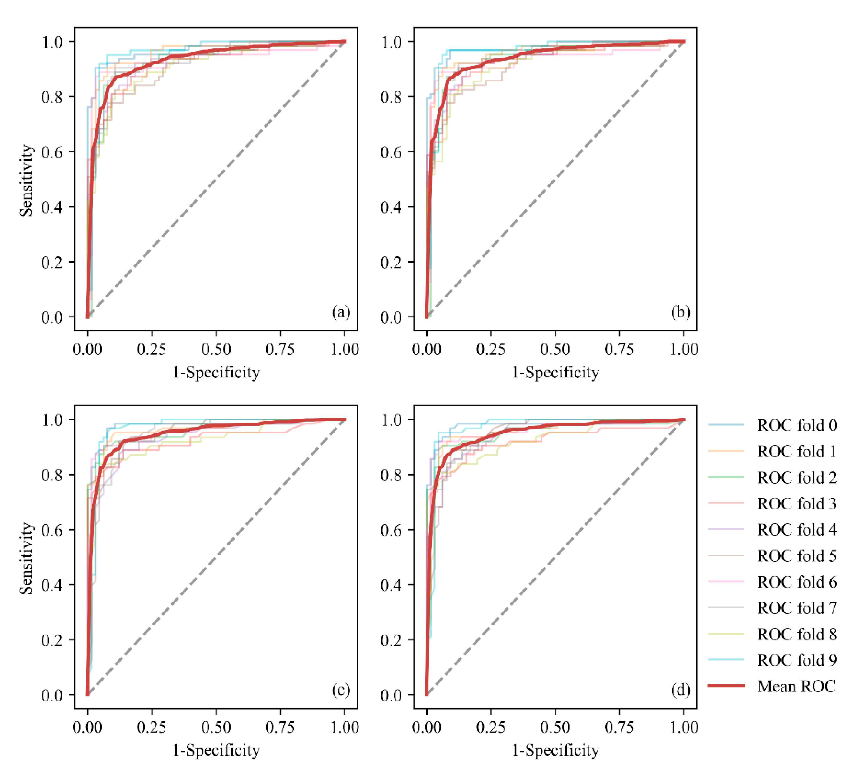
4.3. Model Evaluation

Evaluation is the most important component in modeling; without evaluation results, model outputs lack scientific significance. In this study, receiver operating characteristic (ROC) curves and the area under the curve (AUC) were used to assess the predictive power of the LR and RF models. The global performance of these models was evaluated using an ROC curve that was constructed based on the true positive rate (sensitivity) and false positive rate (specificity):

$$\mathrm{Sensitivity}=\frac{\mathrm{TP}}{\mathrm{TP}+\mathrm{FN}}$$

(9)

$$\mathrm{Specificity}=\frac{\mathrm{TN}}{\mathrm{TN}+\mathrm{FP}}$$

(10)

where TP (true positive) and TN (true negative) represent correctly classified samples in the training and validation datasets; FP (false positive) and FN (false negative) represent incorrectly classified samples in the training and validation datasets. To quantify the global performance of the model, an AUC between 0.5 and 1 was also used. A high AUC value indicates that the model displays good predictive capability.

In addition, the model accuracy is widely used to evaluate the predictive abilities of various models; this metric is defined as the ratio of the number of correctly simulated samples (TP and TN) to the total number of samples. The corresponding formula is as follows:

$$\mathrm{Accuracy}=\frac{\mathrm{TP}+\mathrm{TN}}{\mathrm{TP}+\mathrm{FP}+\mathrm{TN}+\mathrm{FN}}$$

(11)

The closer the accuracy is to 1, the better the model performance is.

5. Results

5.1. Selection of Conditioning Factors Based on the Embedded Method

The utilized embedded method selects important features while the model is being trained. To perform EFS, the machine learning algorithms were preliminarily modeled, and the EFS process was implemented using only the training dataset. The models were trained using a 10-fold cross-validation technique that fully utilized the available data. In LR, the data should be standardized before modeling so that the regression coefficients can be compared. The key to EFS with the LR and RF models involved the determination of a threshold, and the features below this threshold value were discarded. The threshold was derived from the coefficients in LR and the feature importance in RF. We obtain the optimal threshold by drawing a learning curve that represents the change in the mean accuracy obtained after 10-fold cross-validation with different threshold values. The learning curve represents the variation in the results obtained by cross-validating the models with different quantitative features. The LR and RF learning curves are shown in Figure 5. The threshold ranges from 0 to the maximum coefficient or feature importance value. The feature selection results obtained with LR correspond to a threshold range of 0 to 0.25, showing better results than those obtained using all features; similarly, the RF feature selection results correspond to a threshold range of 0 to 0.01. The optimal threshold value for LR was found to be 0.11, and 32 features were selected. The mean accuracy of the features obtained by EFS (0.8844) was obviously higher than that for all features (0.8719). In addition, the RF model was determined to have an optimal threshold value of 0.004, and 28 features were selected. EFS likewise provided a higher mean accuracy (0.8961) than obtained when using all features (0.8891).

We also compared the model performance obtained using all features and EFS by analyzing the mean AUC. The ROC curves derived after the 10-fold cross-validation of the LR and RF models are shown in Figure 6. For LR, the mean AUC of EFS (0.9366) was higher than that obtained using all features (0.9312). Likewise, for the RF model, the mean AUC of EFS (0.9474) was also higher than that using all features (0.9466).

5.2. Model Validation and Comparison

The test datasets were used to estimate the predictive abilities of the two models. The ROC curves of the two models combining EFS illustrate the prediction rates (Figure 7). The ROC assessment of the LR model revealed an AUC value of 0.9277 for the prediction rate, and the accuracy of the LR model was 0.8634. The RF model exhibited better overall performance than the LR model, as reflected in its AUC and accuracy values of 0.9486 and 0.8834, respectively. In addition, the performance of the two models after feature selection was compared on the training set for ten-fold cross-validation versus on the test set (

Table 1. Classification performance of training and test sets of LR and RF models.

		LR		RF
		Accuracy	AUC	Accuracy	AUC
Train data	Fold 1	0.9147	0.9726	0.9302	0.9790
	Fold 2	0.9140	0.9604	0.9218	0.9614
	Fold 3	0.8828	0.9304	0.8906	0.9552
	Fold 4	0.8593	0.9270	0.8593	0.9181
	Fold 5	0.8671	0.9372	0.8593	0.9407
	Fold 6	0.8437	0.9131	0.8984	0.9471
	Fold 7	0.9062	0.9270	0.9218	0.9603
	Fold 8	0.8828	0.9433	0.875	0.9501
	Fold 9	0.8281	0.9140	0.8515	0.9162
	Fold 10	0.9453	0.9626	0.9531	0.9698
	Mean	0.8844	0.9366	0.8961	0.9474
Test data		0.8634	0.9277	0.8834	0.9486

). The evaluation metrics of both the training and test sets were close. This means that the model not only fits the training set, but also successfully generalizes to the test set and achieves similar precision. Therefore, the model was not overfitted to the training set resulting in poor precision in the test set. Meanwhile, the model can maintain a stable performance under different data sets, indicating that the model is more tolerant to data variations with robustness.

The conditioning factor datasets obtained by EFS for the two models and the importance of the selected features are shown in Figure 8. Here, 32 features were screened for the LR model, and 28 features were screened for the RF model based on the chosen EFS approaches. The importance of the features selected in the LR model was measured by the coefficient of each feature, and the importance of the features selected in the RF model was determined using the contribution of the feature to the trees in the model. The results indicate that the features selected in the LR model are similar to those selected in the RF model. Continuous features, such as the elevation, slope, plan curvature, profile curvature, TRI, CI, TWI, distance to rivers, stream density, NDVI, and MSP, were selected in both models. The curvature, SPI, and MAP were considered to make major contributions in the RF model but not in the LR model. In terms of categorical features, the landform, land use, lithology, and soil type were selected for the two models. The southeastern slope class was selected in the LR model, and no aspect classes were used for the RF model. Although the selected features in the two models are similar, the importance of these features to the models is quite different. The LR model is partial to the binary features generated by one-hot encoding; in contrast, the RF model considers continuous features to be more important. Eight of the top-ten features listed in the feature importance indices of the LR model were binary features, while the opposite was true for the RF model (Figure 8). Among the factors screened by EFS in the LR model, tundra and the artificial surface land use class are the most important. However, the RF model results indicate that the NDVI and MAP are the most important factors.

5.3. Generating FFSMs

The flash flood susceptibility indices were calculated using the LR and RF models, and subsequently, FFSMs were generated in a geographic information system (GIS) environment. The flash flood susceptibility indices ranged from 0 to 1; high values indicate high flash flood probabilities. It is necessary to categorize susceptibility maps using appropriate classification methods to intuitively display flash flood susceptibility results. We divided the final susceptibility maps into five classes based on an approach used in other studies [10,44]: very low, low, moderate, high and very high susceptibility. Among the many existing classification methods, the quantile method [14,41,56,57] and natural breaks method [9,24,58] are the most popular. We tested both methods to classify into susceptibility maps of LR and RF separately. In general, it is more reasonable for considerable flash flood points falling into high or very high susceptibility areas.

Table 2. Numbers of historical flash flood events that occurred in regions with various susceptibility classes.

Susceptibility Classes	LR		RF
	Quantile	Nature Breaks	Quantile	Nature Breaks
Very low	3	3	3	5
Low	8	11	2	3
Moderate	21	23	1	16
High	52	50	11	63
Very high	831	828	898	828

shows that fewer flash flood points are classified into the very low and low susceptibility classes by quantile method either in the LR or RF models. Hence, the quantile method is considered more accurate than the natural breaks method for the data used in this study. Figure 9 shows the final susceptibility maps obtained using the two models. There are obvious and large flash flood-prone areas in the southern and southwestern regions of the study area, and areas close to rivers also display high flash flood susceptibility.

Moreover, the pixel-level statistics for the FFSMs obtained with the two models were calculated (Figure 10). The statistical results of the two models differ to some extent. Compared with that of the LR model, the FFSM of the RF model exhibited more fluctuating pixel distributions for all classes. Extreme susceptibility classes, such as the very low and very high susceptibility classes, included fewer pixels, while the moderate and low susceptibility classes had the most pixels. However, the pixel counts of the two models were similar for the high-susceptibility class.

Furthermore, the classification results for the two susceptibility maps were statistically analyzed, and a heatmap and spatial distribution map were constructed (Figure 11). The cross-statistics among the susceptibility classes were used to obtain the corresponding pixel proportions, which were displayed in the heatmap. The percentage of pixels with consistent susceptibility classification in the two models was 41.82%, and the results obtained for the very-high-susceptibility class exhibited the highest consistency between the two maps. More classification differences were obtained between neighboring grades, and the larger the discrepancy between grades was, the smaller the classification difference was. To compare the spatial discrepancies between the results output by the two models, the two FFSMs were superimposed. There were 25 correspondences, and the colors in the heatmap were assigned accordingly. Because many pixels fall within the same or adjacent susceptibility classes, the color near the diagonal line in the heatmap is darkest. Similarly, the darker the color area in the spatial distribution map is, the higher the consistency between the results of the two models. The spatial distribution map is dark overall. There are obvious light-colored areas along the mainstream of the Songhua River in the middle of the study area and in the southernmost area, and in the west, central and south regions, dark-colored areas can be observed.

6. Discussion

At present, flash flood susceptibility research has received extensive attention, and various models have been applied in the field. However, no uniform standard has been established regarding the method for selecting the features input into models. The preparation of a large number of features is conducive to obtaining predictions using machine learning algorithms; thus, we integrated features selected in other studies and used more features for the calculations performed in this study. However, the inclusion of redundant features reduces the prediction efficiency; therefore, feature selection is necessary, especially when many features are present. In this study, EFS was adopted to select feature sets for LR and RF models. The results show that EFS can remove features that contribute less to the predictions while maintaining or even improving the model results. Simultaneously, embedded methods select features from original factor datasets that are specific to the utilized models. Unlike in previous studies [5,9,16], in this study, the LR and RF models were run using different feature sets.

The primary objective of the present study was to generate reliable FFSMs of the mainstream basin of the Songhua River using two machine learning approaches. The applied LR and RF approaches have been widely used in flash flood susceptibility assessments [20,56,59]. The performance of the two models was evaluated and compared using accuracy and AUC values in this study. The AUC values indicated that both the LR and RF models were accurate for estimating flash flood susceptibility in the study area, and these results were supported by those reported in similar studies. At the national scale, Zhao et al. [20] reported AUC values of approximately 0.84 and 0.76 for training and testing datasets, respectively, in mountainous areas of China. Chen et al. [59] obtained AUC values of 0.951 and 0.925 in their model construction and validation processes, respectively, using the RF method in Quannan County, China. RF methods have also been shown to display good learning and predictive abilities in other studies [12,57,60]. Similarly, the results obtained in this study ultimately indicate that the RF model was superior to the LR model when modeling flash flood susceptibility in the study area. However, in contrast to the results of other studies [12,61], the AUC and accuracy values of the two models did not differ extensively in this study, and all values could be considered acceptable for predicting flash flood susceptibility. This result may be related to the specific optimal feature sets of the two models. Instead of using the same feature set for multiple models, more appropriate feature sets were selected for the two models individually to improve the model accuracies. By combining previous research with the results of the present study, RF modeling is found to have application potential for assessing flash flood susceptibility using biophysical characteristics. The clear drawback of the RF method is that it is a “black box” model because individual classification trees are difficult to examine separately [62]. Moreover, it is difficult to provide confidence intervals and regression coefficients for the RF model [63]. This method could thus cause complications if applied by basin managers who are not specifically trained in nonparametric techniques.

The strength and direction of the relationships among flash flood factors may vary as a function of the chosen model. In other words, the same biophysical variable may make different contributions depending on the utilized model, and our study supports this result. To further compare the feature preference differences between the two models used in this study, the importance parameters of each model were used to evaluate the feature importance after modeling. The linear model, LR, and nonlinear model, RF, exhibited very different feature requirements. As LR is a generalized linear model, it more easily calculates and expresses binary features. Therefore, the binary features generated by one-hot encoding had a certain influence on the feature importance evaluation results. Significantly, compared to the RF model, binary features ranked higher in feature importance of the LR model. However, we also found some similarities between the two models; for example, the feature sets selected for the two models shared 21 common features. Among the continuous features, the NDVI and distance to rivers were of high importance to the two models, as were forest (land use 20) and tundra (land use 70) variables among the binary features. The NDVI, forest (land use 20), and tundra (land use 70) features all indicate that vegetation cover is an important factor that affects flash floods in this study area, mainly because dense vegetation cover enhances interception and reduces splash erosion and infiltration [22]. Features that affect certain hydrological processes, such as infiltration, evapotranspiration, and runoff generation, may increase the risk of flash floods. Artificial surfaces (land use 80), which are often composed of impervious surfaces, increase storm runoff and flooding [13,15]. The distance to rivers was identified as another key factor in the models, and this result was consistent with the findings of many other studies [14,16,56]. The susceptibility maps obtained for the studied basin also confirmed this result; notably, higher susceptibility was identified near rivers (Figure 9). MAP and MSP play important roles in model prediction because flash floods are usually driven by high-intensity and short-duration storms [5,64]. Although a more in-depth analysis could be conducted to identify the variables that fluctuate the most between these two models, the small predictive differences obtained for the two models suggest that the influence of the conditioning factors used to estimate the flash flood probability is spatially stable.

Susceptibility is an important scientific topic that has been researched by scholars. The construction of FFSMs is a crucial step in the management of flood disasters in river basins. Through the analysis of the two FFSMs obtained in this study and the resulting spatial distribution map, which display overall dark colors, the results of the two models can be considered consistent overall, and the differences in susceptibility classes are mainly reflected in the adjacent levels. The differences displayed in the map resulted from differences in the model preferences and feature importance assessments. For example, in areas along rivers, the obvious light colors indicate that the prediction results of the LR and RF models are quite different here. This result was likely obtained because the distance to rivers was considered more important by the RF model than by the LR model. Differences in obtained susceptibility maps exist in many susceptibility studies, even when the same feature set is used [9,10,24]. Therefore, the FFSMs obtained from different models should be applied synergistically. In our study area, areas that are highly susceptible to flash floods are concentrated near rivers and in some regions in the southwestern part of the region. This is also consistent with the spatial distribution of historical flash flood events (Figure 1). The susceptibility is predicted based on the information provided by historical flash flood events, and regions with frequent flash floods in the past usually present high susceptibility rank on the susceptibility map. The generated FFSMs quantitatively assesses the susceptibility level of the study area, which can provide a reference for flood control and disaster management in the study area. Areas with high and very high susceptibility should be given more attention than other areas. In addition, the conditioning factor datasets obtained for the two models used in this study can provide data references for future related studies conducted in this region to simplify data collection.

7. Conclusions

In this study, we presented a comparison of the FFSMs obtained using the LR and RF models and focused on the demand for input features in their modeling process, as the selection of features generally has a significant impact on the modeling results but has not received much attention in this field. The impact here includes the precision of the model, the contribution of each factor to the model, the distribution of the final FFSM, and so on. Embedded methods were successfully used to identify the subset of features that contribute the most to the occurrence of flash floods and to improve the accuracy of the FFSMs obtained using LR and RF models to some extent in this study. The two models exhibit similarities as well as differences in terms of feature selection. The similarities resulted from the stability of the regional factors that affect flash floods, and the differences were related to the unique mechanisms of the two models. The binary features implemented in the LR model were considered favorable factors for the construction of the corresponding FFSM. Moreover, the RF model results indicated that interval features play major roles in affecting the susceptibility of an area to flash floods. In fact, the differences between the two models analyzed herein can motivate modelers to consider the available data when selecting a specific model to obtain an FFSM. Moreover, the construction of FFSMs is an urgent task that needs to be accomplished in the main river basin of the Songhua River in Northeast China. This region is a representative region that is highly prone to flash floods. According to the ROC curves and AUC values, both models exhibited accurate and reliable performance in constructing FFSMs; however, the RF model provided a higher predictive capability than the LR model. This study may provide useful information for risk management in flash flood-prone basins and provide a reference for model feature selection in susceptibility studies.

References

- Fang, Z.C.; Wang, Y.; Peng, L.; Hong, H.Y. Predicting flood susceptibility using LSTM neural networks. J. Hydrol. 2020, 594, 125734. [Google Scholar] [CrossRef]
- Milly, P.C.D.; Wetherald, R.T.; Dunne, K.A.; Delworth, T.L. Increasing risk of great floods in a changing climate. Nature 2002, 415, 514–517. [Google Scholar] [CrossRef] [PubMed]
- Schiermeier, Q. Increased flood risk linked to global warming. Nature 2011, 470, 315. [Google Scholar] [CrossRef] [PubMed]
- Destro, E.; Amponsah, W.; Nikolopoulos, E.I.; Marchi, L.; Marra, F.; Zoccatelli, D.; Borga, M. Coupled prediction of flash flood response and debris flow occurrence: Application on an alpine extreme flood event. J. Hydrol. 2018, 558, 225–237. [Google Scholar] [CrossRef]
- Bui, D.T.; Ngo, P.T.T.; Pham, T.D.; Jaafari, A.; Minh, N.Q.; Hoa, P.V.; Samui, P. A novel hybrid approach based on a swarm intelligence optimized extreme learning machine for flash flood susceptibility mapping. Catena 2019, 179, 184–196. [Google Scholar] [CrossRef]
- Costache, R.; Pham, Q.B.; Sharifi, E.; Linh, N.T.T.; Abba, S.I.; Vojtek, M.; Vojtekova, J.; Nhi, P.T.T.; Khoi, D.N. Flash-Flood Susceptibility Assessment Using Multi-Criteria Decision Making and Machine Learning Supported by Remote Sensing and GIS Techniques. Remote Sens. 2019, 12, 106. [Google Scholar] [CrossRef]
- Ahmadalipour, A.; Moradkhani, H. A data-driven analysis of flash flood hazard, fatalities, and damages over the CONUS during 1996–2017. J. Hydrol. 2019, 578, 124106. [Google Scholar] [CrossRef]
- Costache, R.; Bui, D.T. Identification of areas prone to flash-flood phenomena using multiple-criteria decision-making, bivariate statistics, machine learning and their ensembles. Sci. Total Environ. 2020, 712, 136492. [Google Scholar] [CrossRef]
- Arabameri, A.; Saha, S.; Chen, W.; Roy, J.; Pradhan, B.; Bui, D.T. Flash flood susceptibility modelling using functional tree and hybrid ensemble techniques. J. Hydrol. 2020, 587, 125007. [Google Scholar] [CrossRef]
- Costache, R.; Pham, Q.B.; Avand, M.; Linh, N.T.T.; Vojtek, M.; Vojtekova, J.; Lee, S.; Khoi, D.N.; Nhi, P.T.T.; Dung, T.D. Novel hybrid models between bivariate statistics, artificial neural networks and boosting algorithms for flood susceptibility assessment. J. Environ. Manag. 2020, 265, 110485. [Google Scholar] [CrossRef]
- Bui, D.T.; Tuan, T.A.; Klempe, H.; Pradhan, B.; Revhaug, I. Spatial prediction models for shallow landslide hazards: A comparative assessment of the efficacy of support vector machines, artificial neural networks, kernel logistic regression, and logistic model tree. Landslides 2016, 13, 361–378. [Google Scholar] [CrossRef]
- Trigila, A.; Iadanza, C.; Esposito, C.; Scarascia-Mugnozza, G. Comparison of Logistic Regression and Random Forests techniques for shallow landslide susceptibility assessment in Giampilieri (NE Sicily, Italy). Geomorphology 2015, 249, 119–136. [Google Scholar] [CrossRef]
- Rahmati, O.; Pourghasemi, H.R.; Zeinivand, H. Flood susceptibility mapping using frequency ratio and weights-of-evidence models in the Golastan Province, Iran. Geocarto Int. 2016, 31, 42–70. [Google Scholar] [CrossRef]
- Tehrany, M.S.; Pradhan, B.; Mansor, S.; Ahmad, N. Flood susceptibility assessment using GIS-based support vector machine model with different kernel types. Catena 2015, 125, 91–101. [Google Scholar] [CrossRef]
- Tehrany, M.S.; Pradhan, B.; Jebur, M.N. Spatial prediction of flood susceptible areas using rule based decision tree (DT) and a novel ensemble bivariate and multivariate statistical models in GIS. J. Hydrol. 2013, 504, 69–79. [Google Scholar] [CrossRef]
- Khosravi, K.; Pham, B.T.; Chapi, K.; Shirzadi, A.; Shahabi, H.; Revhaug, I.; Prakash, I.; Bui, D.T. A comparative assessment of decision trees algorithms for flash flood susceptibility modeling at Haraz watershed, northern Iran. Sci. Total Environ. 2018, 627, 744–755. [Google Scholar] [CrossRef]
- Choubin, B.; Moradi, E.; Golshan, M.; Adamowski, J.; Sajedi-Hosseini, F.; Mosavi, A. An ensemble prediction of flood susceptibility using multivariate discriminant analysis, classification and regression trees, and support vector machines. Sci. Total Environ. 2019, 651, 2087–2096. [Google Scholar] [CrossRef]
- Chen, W.; Xie, X.S.; Wang, J.L.; Pradhan, B.; Hong, H.Y.; Bui, D.T.; Duan, Z.; Ma, J.Q. A comparative study of logistic model tree, random forest, and classification and regression tree models for spatial prediction of landslide susceptibility. Catena 2017, 151, 147–160. [Google Scholar] [CrossRef]
- Bui, D.T.; Hoang, N.D.; Martinez-Alvarez, F.; Ngo, P.T.T.; Hoa, P.V.; Pham, T.D.; Samui, P.; Costache, R. A novel deep learning neural network approach for predicting flash flood susceptibility: A case study at a high frequency tropical storm area. Sci. Total Environ. 2019, 701, 134413. [Google Scholar] [CrossRef]
- Zhao, G.; Pang, B.; Xu, Z.X.; Yue, J.J.; Tu, T.B. Mapping flood susceptibility in mountainous areas on a national scale in China. Sci. Total Environ. 2018, 615, 1133–1142. [Google Scholar] [CrossRef]
- Hong, H.Y.; Tsangaratos, P.; Ilia, I.; Liu, J.Z.; Zhu, A.X.; Chen, W. Application of fuzzy weight of evidence and data mining techniques in construction of flood susceptibility map of Poyang County, China. Sci. Total Environ. 2018, 625, 575–588. [Google Scholar] [CrossRef] [PubMed]
- Panahi, M.; Dodangeh, E.; Rezaie, F.; Khosravi, K.; Le, H.V.; Lee, M.J.; Lee, S.; Pham, B.T. Flood spatial prediction modeling using a hybrid of meta-optimization and support vector regression modeling. Catena 2021, 199, 105114. [Google Scholar] [CrossRef]
- Guyon, I.; Elisseeff, A. An introduction to variable and feature selection. J. Mach. Learn. Res. 2003, 3, 1157–1182. [Google Scholar] [CrossRef][Green Version]
- Bui, D.T.; Tsangaratos, P.; Ngo, P.T.T.; Pham, T.D.; Pham, B.T. Flash flood susceptibility modeling using an optimized fuzzy rule based feature selection technique and tree based ensemble methods. Sci. Total Environ. 2019, 668, 1038–1054. [Google Scholar] [CrossRef] [PubMed]
- Zheng, A.; Casari, A. Feature Engineering for Machine Learning; Roumeliotis, R., Bleiel, J., Eds.; O’Reilly Media, Inc.: Sebastopol, CA, USA, 2018. [Google Scholar]
- Chen, C.; Tsai, Y.; Chang, F.; Lin, W. Ensemble feature selection in medical datasets: Combining filter, wrapper, and embedded feature selection results. Expert Syst. 2020, 37, e12553. [Google Scholar] [CrossRef]
- Yu, L.; Liu, H. Efficient Feature Selection via Analysis of Relevance and Redundancy. J. Mach. Learn. Res. 2004, 5, 1205–1224. [Google Scholar] [CrossRef]
- Saeys, Y.; Inza, I.; Larrañaga, P. A review of feature selection techniques in bioinformatics. Bioinformatics 2007, 23, 2507–2517. [Google Scholar] [CrossRef]
- Chandrashekar, G.; Sahin, F. A survey on feature selection methods. Comput. Electr. Eng. 2014, 40, 16–28. [Google Scholar] [CrossRef]
- Rodriguez-Galiano, V.F.; Luque-Espinar, J.A.; Chica-Olmo, M.; Mendes, M.P. Feature selection approaches for predictive modelling of groundwater nitrate pollution: An evaluation of filters, embedded and wrapper methods. Sci. Total Environ. 2018, 624, 661–672. [Google Scholar] [CrossRef]
- Liang, P.; Qin, C.Z.; Zhu, A.X.; Hou, Z.W.; Fan, N.Q.; Wang, Y.J. A case-based method of selecting covariates for digital soil mapping. J. Integr. Agric. 2020, 19, 2127–2136. [Google Scholar] [CrossRef]
- Lark, R.M.; Bishop, T.F.A.; Webster, R. Using expert knowledge with control of false discovery rate to select regressors for prediction of soil properties. Geoderma 2007, 138, 65–78. [Google Scholar] [CrossRef]
- Derksen, S.; Keselman, H.J. Backward, forward and stepwise automated subset selection algorithms: Frequency of obtaining authentic and noise variables. Br. J. Math. Stat. Psychol. 1992, 45, 265–282. [Google Scholar] [CrossRef]
- Lal, T.N.; Chapelle, O.; Weston, J.; Elisseeff, A. Embedded Methods. In Feature Extraction: Foundations and Applications; Guyon, I., Nikravesh, M., Gunn, S., Zadeh, L.A., Eds.; Springer: Berlin/Heidelberg, Germany, 2006; pp. 137–165. [Google Scholar]
- Liu, C.J.; Guo, L.; Ye, L.; Zhang, S.F.; Zhao, Y.Z.; Song, T.Y. A review of advances in China’s flash flood early-warning system. Nat. Hazards 2018, 92, 619–634. [Google Scholar] [CrossRef]
- Songliao Water Conservancy Commission. Summary of “Songhua River Basin Comprehensive Planning (2012–2030)”; Songliao Water Conservancy Commission: Changchun, China, 2013. [Google Scholar]
- Liu, Y.; Huang, Y.; Wan, J.; Yang, Z.; Zhang, X. Analysis of Human Activity Impact on Flash Floods in China from 1950 to 2015. Sustainability 2021, 13, 217. [Google Scholar] [CrossRef]
- Hapuarachchi, H.A.P.; Wang, Q.J.; Pagano, T.C. A review of advances in flash flood forecasting. Hydrol. Process. 2011, 25, 2771–2784. [Google Scholar] [CrossRef]
- Bui, D.T.; Pradhan, B.; Nampak, H.; Bui, Q.T.; Tran, Q.A.; Nguyen, Q.P. Hybrid artificial intelligence approach based on neural fuzzy inference model and metaheuristic optimization for flood susceptibilitgy modeling in a high-frequency tropical cyclone area using GIS. J. Hydrol. 2016, 540, 317–330. [Google Scholar] [CrossRef]
- Pham, B.T.; Avand, M.; Janizadeh, S.; Phong, T.V.; Al-Ansari, N.; Ho, L.S.; Das, S.; Le, H.V.; Amini, A.; Bozchaloei, S.K.; et al. GIS Based Hybrid Computational Approaches for Flash Flood Susceptibility Assessment. Water 2020, 12, 683. [Google Scholar] [CrossRef]
- Khosravi, K.; Shahabi, H.; Pham, B.T.; Adamowski, J.; Shirzadi, A.; Pradhan, B.; Dou, J.; Ly, H.B.; Grof, G.; Ho, H.L.; et al. A comparative assessment of flood susceptibility modeling using Multi-Criteria Decision-Making Analysis and Machine Learning Methods. J. Hydrol. 2019, 573, 311–323. [Google Scholar] [CrossRef]
- Riley, S.J.; DeGloria, S.D.; Elliot, R. A terrain ruggedness index that quantifies topographic heterogeneity. Intermt. J. Sci. 1999, 5, 23–27. [Google Scholar]
- Costache, R. Flash-Flood Potential assessment in the upper and middle sector of Prahova river catchment (Romania). A comparative approach between four hybrid models. Sci. Total Environ. 2019, 659, 1115–1134. [Google Scholar] [CrossRef]
- Tehrany, M.S.; Pradhan, B.; Jebur, M.N. Flood susceptibility mapping using a novel ensemble weights-of-evidence and support vector machine models in GIS. J. Hydrol. 2014, 512, 332–343. [Google Scholar] [CrossRef]
- Shahabi, H.; Shirzadi, A.; Ghaderi, K.; Omidvar, E.; Al-Ansari, N.; Clague, J.J.; Geertsema, M.; Khosravi, K.; Amini, A.; Bahrami, S.; et al. Flood Detection and Susceptibility Mapping Using Sentinel-1 Remote Sensing Data and a Machine Learning Approach: Hybrid Intelligence of Bagging Ensemble Based on K-Nearest Neighbor Classifier. Remote Sens. 2020, 12, 266. [Google Scholar] [CrossRef]
- Lee, M.J.; Kang, J.E.; Jeon, S. Application of frequency ratio model and validation for predictive flooded area susceptibility mapping using GIS. In Proceedings of the 2012 IEEE International Geoscience and Remote Sensing Symposium, Munich, Germany, 22–27 July 2012; pp. 895–898. [Google Scholar]
- Razavi Termeh, S.V.; Kornejady, A.; Pourghasemi, H.R.; Keesstra, S. Flood susceptibility mapping using novel ensembles of adaptive neuro fuzzy inference system and metaheuristic algorithms. Sci. Total Environ. 2018, 615, 438–451. [Google Scholar] [CrossRef] [PubMed]
- Moore, I.D.; Grayson, R.B.; Ladson, A.R. Digital terrain modelling: A review of hydrological, geomorphological, and biological applications. Hydrol. Process. 1991, 5, 3–30. [Google Scholar] [CrossRef]
- Pan, X.Z.; Pan, K. National 1:4 Million Soil Type Distribution Map (China Soil System Classification System) (2000); National Earth System Science Data Center-Soil Data Center: Nanjing, China, 2015. [CrossRef]
- Waqas, H.; Lu, L.; Tariq, A.; Li, Q.; Baqa, M.F.; Xing, J.; Sajjad, A. Flash Flood Susceptibility Assessment and Zonation Using an Integrating Analytic Hierarchy Process and Frequency Ratio Model for the Chitral District, Khyber Pakhtunkhwa, Pakistan. Water 2021, 13, 1650. [Google Scholar] [CrossRef]
- Pedregosa, F.; Varoquaux, G.; Gramfort, A.; Michel, V.; Thirion, B.; Grisel, O.; Blondel, M.; Prettenhofer, P.; Weiss, R.; Dubourg, V.; et al. Scikit-learn: Machine Learning in Python. J. Mach. Learn. Res. 2011, 12, 2825–2830. [Google Scholar] [CrossRef]
- Jaafari, A.; Mafi-Gholami, D.; Pham, B.T.; Bui, D.T. Wildfire Probability Mapping: Bivariate vs. Multivariate Statistics. Remote Sens. 2019, 11, 618. [Google Scholar] [CrossRef]
- Breiman, L. Random forests. Mach. Learn. 2001, 45, 5–32. [Google Scholar] [CrossRef]
- Liaw, A.; Wiener, M.C. Classification and Regression by RandomForest. R News 2002, 2, 18–22. [Google Scholar]
- Louppe, G. Understanding Random Forests: From Theory to Practice. Ph.D. thesis, University of Liège, Liège, Belgium, 2014. [Google Scholar]
- Chapi, K.; Singh, V.P.; Shirzadi, A.; Shahabi, H.; Bui, D.T.; Pham, B.T.; Khosravi, K. A novel hybrid artificial intelligence approach for flood susceptibility assessment. Environ. Modell. Softw. 2017, 95, 229–245. [Google Scholar] [CrossRef]
- Tang, X.Z.; Li, J.F.; Liu, M.N.; Liu, W.; Hong, H.Y. Flood susceptibility assessment based on a novel random Naive Bayes method: A comparison between different factor discretization methods. Catena 2020, 190, 104536. [Google Scholar] [CrossRef]
- Chen, W.; Hong, H.Y.; Li, S.J.; Shahabi, H.; Wang, Y.; Wang, X.J.; Bin Ahmad, B. Flood susceptibility modelling using novel hybrid approach of reduced-error pruning trees with bagging and random subspace ensembles. J. Hydrol. 2019, 575, 864–873. [Google Scholar] [CrossRef]
- Chen, W.; Li, Y.; Xue, W.F.; Shahabi, H.; Li, S.J.; Hong, H.Y.; Wang, X.J.; Bian, H.Y.; Zhang, S.; Pradhan, B.; et al. Modeling flood susceptibility using data-driven approaches of naive Bayes tree, alternating decision tree, and random forest methods. Sci. Total Environ. 2019, 701, 134979. [Google Scholar] [CrossRef]
- Pahlavan-Rad, M.R.; Dahmardeh, K.; Hadizadeh, M.; Keykha, G.; Mohammadnia, N.; Gangali, M.; Keikha, M.; Davatgar, N.; Brungard, C. Prediction of soil water infiltration using multiple linear regression and random forest in a dry flood plain, eastern Iran. Catena 2020, 194, 104715. [Google Scholar] [CrossRef]
- Guo, F.T.; Wang, G.Y.; Su, Z.W.; Liang, H.L.; Wang, W.H.; Lin, F.F.; Liu, A.Q. What drives forest fire in Fujian, China? Evidence from logistic regression and Random Forests. Int. J. Wildland Fire 2016, 25, 505–519. [Google Scholar] [CrossRef]
- Prasad, A.M.; Iverson, L.R.; Liaw, A. Newer classification and regression tree techniques: Bagging and random forests for ecological prediction. Ecosystems 2006, 9, 181–199. [Google Scholar] [CrossRef]
- Cutler, D.R.; Edwards, T.C.; Beard, K.H.; Cutler, A.; Hess, K.T. Random forests for classification in ecology. Ecology 2007, 88, 2783–2792. [Google Scholar] [CrossRef] [PubMed]
- Borga, M.; Anagnostou, E.N.; Bloschl, G.; Creutin, J.D. Flash flood forecasting, warning and risk management: The HYDRATE project. Environ. Sci. Policy 2011, 14, 834–844. [Google Scholar] [CrossRef]