Abstract
This paper addresses the development of a novel zero-shot learning method for remote marine litter hyperspectral imaging data classification. The work consisted of using an airborne acquired marine litter hyperspectral imaging dataset that contains data about different plastic targets and other materials and assessing the viability of detecting and classifying plastic materials without knowing their exact spectral response in an unsupervised manner. The classification of the marine litter samples was divided into known and unknown classes, i.e., classes that were hidden from the dataset during the training phase. The obtained results show a marine litter automated detection for all the classes, including (in the worst case of an unknown class) a precision rate over 56% and an overall accuracy of 98.71%.
1. Introduction
Nowadays, marine litter is one of the biggest threats to marine ecosystems. The characteristics of the marine litter found in the oceans have changed over the years, and it is made up of human-based plastic waste that is a threat to marine life. To address this problem, the research community is always looking for novel methods, tools and systems to detect, classify and remove marine litter accumulation zones from the sea. For accomplishing this objective, it is important to characterise marine litter, discover its point of origin and help create mitigation strategies to decrease its presence in the oceans [1,2,3,4].
Our research work focuses on the use of hyperspectral imaging systems for remote marine litter detection [5,6]. Despite being an expensive and complex technology, it is robust and can cope better with exogenous situations such as solar reflections, which are a major concern for RGB cameras due to its higher probability of returning a completely saturated image. Hyperspectral imaging systems can collect information of hundreds of wavelengths, from visible to the infrared spectrum range.
Currently most of the earth observation (EO) detection methods for marine litter are based on satellite information [7,8,9,10,11]. Satellites are able to provide lots of information with a good revisiting time over extended areas which makes them an ideal tool for marine litter detection. However, current satellite on-board sensors such as multispectral imaging sensors are not designed for marine litter detection and their spatial resolution and spectral bands information is far from ideal to solve the problem due to the reduced number of available wavelengths.
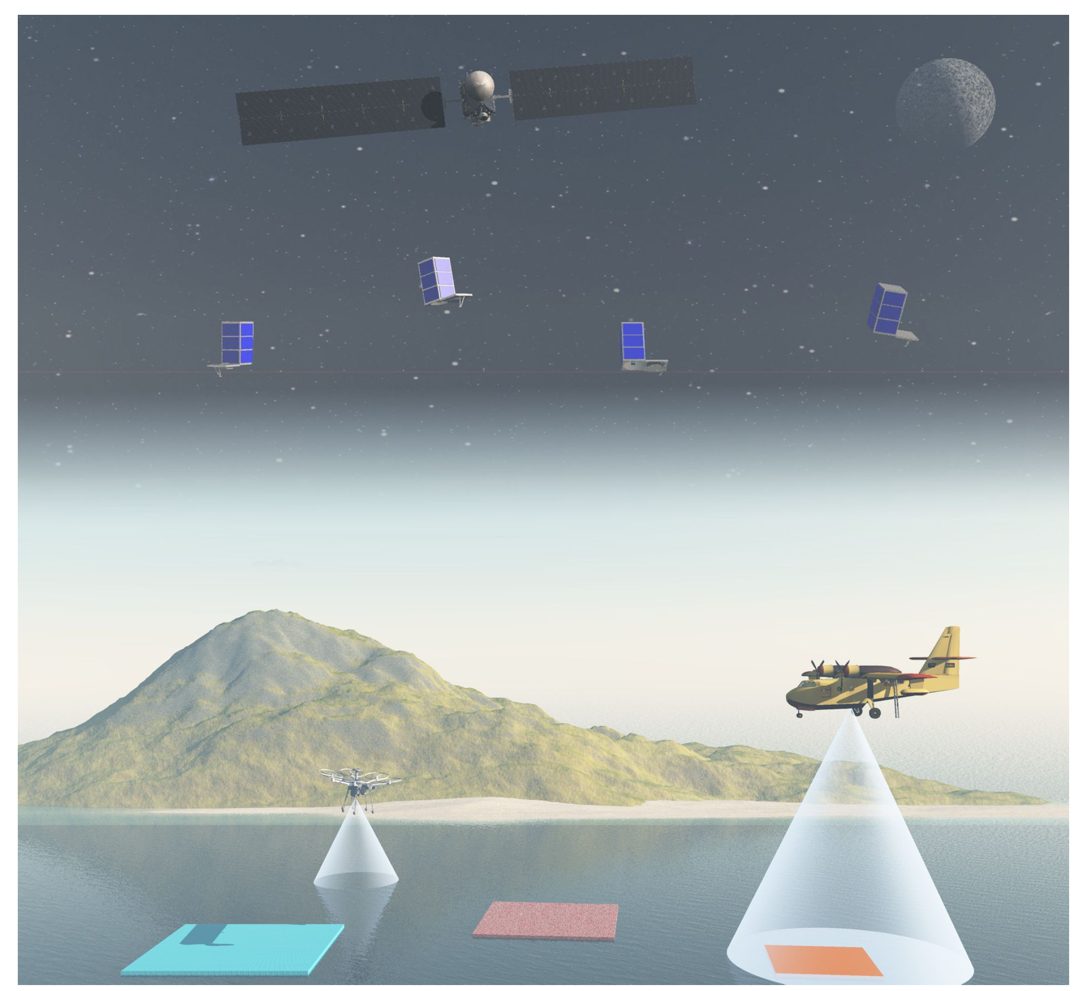
One way to overcome such limitations is by using airborne platforms equipped with hyperspectral imaging systems, which can analyse the requirements at the spatial and spectral data level for future sensors development and provide a remote conceptual framework for marine litter detection as illustrated in Figure 1.

Figure 1.
Conceptual framework for a remote marine litter detection system.
However, even with all the information provided by hyperspectral imaging systems, the problem of detection is still complex due to the number of different plastic materials present in marine litter (multiple spectral analysis). Furthermore, dealing with hyperspectral data is computationally expensive, and it is quite challenging to collect and manually label data for all types of existing plastic marine litter. By resorting to new deep learning methods, such as zero-shot learning (ZSL) approaches, it is possible to create a mixed approach between supervised and unsupervised techniques. We can also fostering a research path that in the future we can resort to in order to detect different plastic materials without an exhaustive manual classification, where the airborne platform equipped with the hyperspectral imaging system can detect and classify in near real time.
Zero-shot learning is a deep learning technique that detects and distinguishes unavailable classes during the training phase. By learning an intermediate semantic layer using the relation between the known and unknown classes, it can apply this at the inference time to predict a new class of data. This is usually completed by projecting the test data to a new space (using regression or classification), and a similarity measure with each unknown class is used for prediction. It has been used in different research areas, such as face verification [12], object recognition [13], video understanding [14,15,16,17] and natural language processing [18].
The taxonomy on ZSL copes with different configurations, namely inductive ZSL [13,19,20,21,22,23,24,25,26,27] and transductive [28,29,30,31,32,33]). There are some variations such as few-shot learning [34,35] (during training, some labelled samples from each unknown class are used) and generalised zero-shot learning [36,37,38].
Up until now, most researched ZSL methods have been applied to visible image (RGB) data. There are advances in ZSL for hyperspectral imaging but are mainly using a Few-Shot learning (FSL) configuration. Examples of FSL methods are presented in [39,40,41]. The first method [39] presents a novel algorithm that uses a transfer learning scheme to share intrinsic representations from the same type of objects in different domains. Other authors [40] display the MDL4OW method, which can classify and reconstruct the data simultaneously. Finally, [41] develops a heterogeneous few-shot learning (HFSL) for hyperspectral imaging classification, resorting to a residual network to extract spectral information and a convolution network to analyse the spatial information.
There are other FSL approaches to tackle specific problems with the data, as in [42], where the authors developed a new method called deep cross-domain few-shot learning (DCFSL) to mitigate the domain shift issue. They resorted to a conditional adversarial domain adaptation strategy and an FSL application strategy to discover transferable knowledge between the classes. The authors of [43] developed the novel Attention-weighted Graph Convolution (AwGCN), where the internal data relationships are explored for semi-supervised label propagation. Meanwhile, the work of [44] shows a novel approach to mitigate over-fitting by using an auxiliary set of unlabeled samples with soft pseudo-labels to enhance the feature extractor training on a few labeled samples. A more recent work [45] proposes a novel outlier calibration network (OCN) combined with a feature extraction module integrated into the meta-training phase. This feature extraction module comprises a novel residual 3D convolutional block attention network (R3CBAM) for improving spectral–spatial feature learning. This novel approach focuses on the few-shot open-set recognition problem and uses a Variational Autoencoder (VAE) to augment the query set.
In [46], a novel approach for signal recognition, SR2CNN, is developed based on a generalised zero-shot learning approach. The method is divided into four components: feature extractor, classifier, decoder, and discriminator. The algorithm can learn a representation of signal semantic feature space by combining cross-entropy loss, centre loss, and reconstruction loss. This allows discriminating signals not seen during the training phase and improves itself by creating new classes with unseen signals.
The work presented in this paper contributes to the ongoing research efforts to use new unsupervised algorithms for marine litter detection and classification. Our work follows the work developed in [46] but updates the method to cope with hyperspectral imaging data (spectral) and introduces a novel attention layer mechanism to extract meaningful information from the data.
Summarising, the main contributions of this work are:
- A ZSL approach for hyperspectral data, using purely spectral information, that is able to classify pixel by pixel regardless of its shape, which is usually affected by sun exposure and erosion caused by water and rocks;
- This ZSL approach is based on a generalised methodology, which means that it is trained with the known classes, and the classification is performed in all classes, known and unknown. The algorithm is adaptable, meaning that it can classify the samples from unknown classes into different classes;
- The algorithm is tested and evaluated using a real hyperspectral imaging dataset, holding marine litter data acquired during field experiments in Porto Pim bay, Faial island, Azores.
This paper is organised as follows: Section 2 describes the hyperspectral generalised zero-shot learning algorithm, and Section 3 describes the marine litter dataset and the experimental setup. Section 4 presents the results, and Section 5 contains the discussion. The final section draws some conclusions on the work carried out and describes future work.
2. Hyperspectral Zero-Shot Learning Method
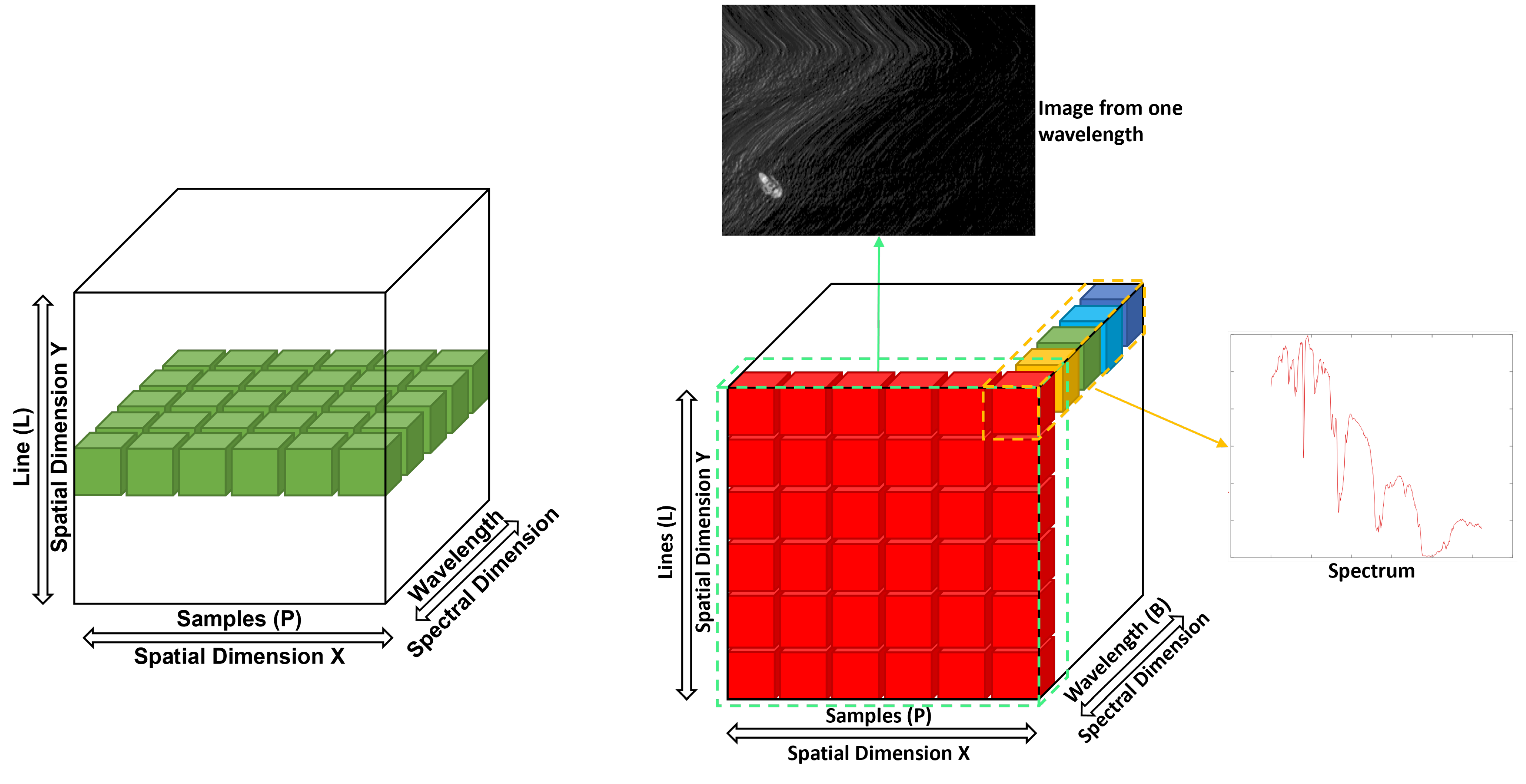
Hyperspectral imaging systems can acquire data using different formats. Our data were acquired resorting to pushbroom hyperspectral cameras, which acquire data simultaneously for each pixel line by line. By combining all the lines, it is possible to obtain a hyperspectral cube represented by a 3D matrix of spectral pixels that can be represented by , where L is the number of lines, P is the number of pixels and W is the number of wavelengths. Each pixel will contain the spectra with the responses in each wavelength, and each pixel will belong to a class assigned by visual inspection. Figure 2 shows a scheme of the data acquired in a single frame using a pushbroom hyperspectral system.

Figure 2.
Acquisition scheme for pushbroom hyperspectral cameras: the left image shows the data that are acquired in each frame, in the case of the hyperspectral system, this is denominated as a line, and it is comprised by all the samples (pixels) and all the bands for each pixel in that line. The right image displays the information that is possible to extract from the hyperspectral cube.
The data acquisition was completed in the radiance domain, from 400 to 2500 nm. The pre-processing of the data is composed of two main steps: normalisation and dimensionality reduction. The first allowed us to normalise the data to have zero mean. The second was needed due to the amount of data and because not all bands contribute equally to the detection of the marine litter samples. In this case, the method used was Principal Component Analysis (PCA) [47], reducing the number of utilised bands from 524 to 64 PCA bands.
Generalised zero-shot learning (GZSL) solves the problem of classic ZSL approaches, where the prediction step consists of using unknown samples. In this case, our training dataset is composed of multiple spectra, each corresponding to one pixel of the pushbroom hyperspectral data cube, all belonging to known classes. Then, the prediction will also have the unknown classes of which the model has no information and has never seen. Let denote the known classes, while represents the unknown class labels, in which X and Y are the input and the output space, respectively. The input is composed of the , while the output is composed of and . In the GZSL, , with . Given the training data, where belongs to X and the label belongs to , the goal is to extrapolate and recognise the spectra in Y. This algorithm can predict the label from sample , where Y contains both known and unknown classes. The algorithm aims to extract semantic information about X, recognise K, and extrapolate to U, by mapping the training space X into a semantic space Z, and then, this semantic encoding is mapped to a class label.
This approach is an updated and enhanced version of the work presented in [46], and it is composed of four different components:
- Feature Extractor (F)—Convolutional Neural Network (CNN), with channel attention modules after each convolutional block [48];
- Classifier (C)—Fully Connected Neural Network;
- Decoder (D)—Autoencoder;
- Discriminator (P).
The first three components, F, C, and D, are used to build a spectral semantic space. Figure 3 shows a scheme for these blocks, while the following sections describe each one in detail.
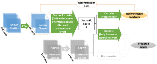
Figure 3.
Schematic of the algorithm used: first, the PCA method is used to reduce the data dimensionality for both the training and prediction phase. To train the algorithm, first, a feature extractor with channel attention modules after each convolutional layer is used to create a semantic space Z. Then, this semantic space is used for the classifier, a fully connected neural network, and by the decoder to create a reconstructed spectrum. To perform the prediction, both the classifier and the discriminator are used, giving a predicted label to each pixel.
2.1. Feature Extractor
The input signal consists of one row with 64 PCA bands. The Feature Extractor (F) module comprises a CNN architecture with four convolutional layers and three fully connected layers. After each convolutional block, a channel attention module improves the CNN architecture. This channel attention module is one part of the well-known Convolutional Block Attention Module (CBAM) [48], given that, in this case, there is no improvement in using both components of CBAM. To minimise the intra-class variations in space Z and, simultaneously, maintain the inter-classes semantic features separated, this component resorts to centre loss [49]. Assuming that batch size is represented by B, and that , with label , so , the centre loss is given by Equation (1), where corresponds to the semantic centre vector of the class in Z, and will be updated according to the class semantic features changes.
Given the limitations with the amount of hyperspectral data, the training dataset will be analysed in batches, which makes updated according to , where denotes the learning rate and can be obtained with Equation (2), where is equal to 1 if the condition is true and 0 otherwise.
2.2. Classifier
The classifier, C, discriminates between the sample labels based on semantic features and comprises several fully connected layers. In this case, we used the cross-entropy loss defined in Equation (3), where is the prediction for the sample .
2.3. Decoder
The decoder is composed of an autoencoder, using deconvolutions, unpolling, and fully connected layers. This component allows the reconstruction of the signal from the latent space Z, using the reconstruction loss to analyse the difference between the input and reconstructed signals. The loss is obtained with Equation (4), where corresponds to the input signal reconstructed.
The total loss function combining all the losses can be expressed as Equation (5).
2.4. Discriminator
Given the latent space Z, the discriminator can distinguish between known and unknown classes by using Equation (6) with the feature extractor F for each known class k, obtaining the semantic centre vector for each known class, where m represents the number of training samples.
when a test spectrum Q is considered and is obtained, the difference between and is measured for each known class k. This distance is obtained by using the Mahalanobis distance with Equation (7), where corresponds to the covariance matrix of semantic features of signals of class k, transformation matrix associated to class k, and is the inverse matrix of .
Given this distance, , it is possible to distinguish between known and unknown classes. This is performed by comparing the threshold with the minimal distance given by Equation (8), where H corresponds to the set of known semantic centre vectors.
Considering that represents the prediction of Q, if , otherwise , where is given by Equation (9), where is the discrimination coefficient.
However, if Q is classified as unknown in the previous step, it is necessary to understand if it will be part of a new class or must be combined with another class. If R refers to the recorded unknown classes, and refers to the set of semantic centre vectors of R, if , a new class label is added to R and is set to be the semantic centre vector . The unknown spectrum Q of an unknown class is saved in set and . If , the threshold defined in Equation (11), which is based on the distance between and , is compared to the minimal distance defined in Equation (10).
Considering that corresponds to the number of record spectrum labels registered in R, and if , a new spectrum label is added to R and set . Given that has no restriction, the model never knows the number of unknown classes left to be discriminated. If , then and the spectrum Q is saved in . The is updated using Equation (12), where corresponds to the number of spectra in the set .
Using this discriminator, the model can distinguish test samples into classes, where is the number of unknown classes distinguished by the model.
3. Marine Litter Dataset Acquisition and Experimental Setup
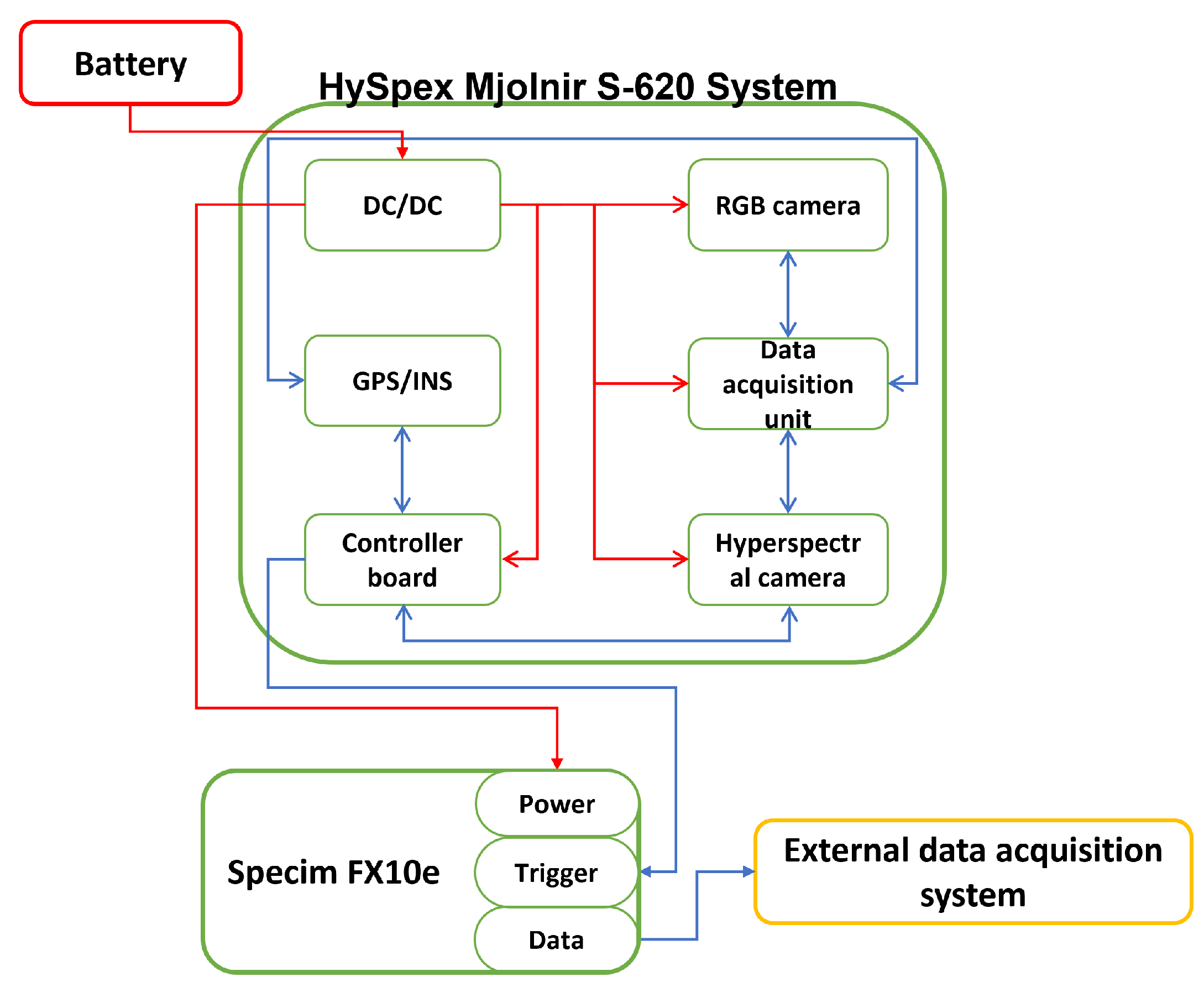
The remote sensing of marine litter with hyperspectral systems from visible to the SWIR range is scarce, a series of issues related to the price of the systems and airborne campaign make it difficult to find available open-source data, and most of the datasets available are from satellite data. Therefore, we resort to a hyperspectral imaging system setup composed of two pushbroom cameras: a Specim FX10e (1024 spatial pixels, spectral range from 400 to 1000 nm) and a HySpex Mjolnir S-620 (620 spatial pixels, spectral range from 970 to 2500 nm). The second camera was inserted into an off-the-shelf system, including a CPU unit, GPS, and an inertial system. Both cameras were synchronised by the HySpex system, controlled by the GPS/INS unit (Applanix APX-15 UAV). Regarding the data acquisition, both cameras acquire data in a raw format that is afterwards calibrated and converted to radiance by the camera manufacturers software, removing the effects of the sensor during the acquisition. The connections between the multiple components of these system are shown in Figure 4, and it is possible to find a detailed description about each module in [5,6].
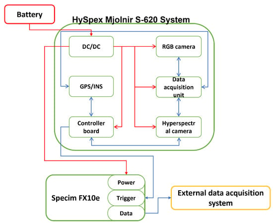
Figure 4.
Hyperspectral imaging system hardware connections.
The hyperspectral imaging system was then installed in a Cessna aircraft, F-BUMA, as shown in Figure 5, where it is possible to see the airplane, and the payload is already mounted on the airplane landing gear. For the dataset acquisition, the flight altitude was around 600 m above sea level.

Figure 5.
On the left-hand side image, the F-BUMA aircraft, and on the right side of the image, the hyperspectral imaging payload installation on aircraft landing gear.
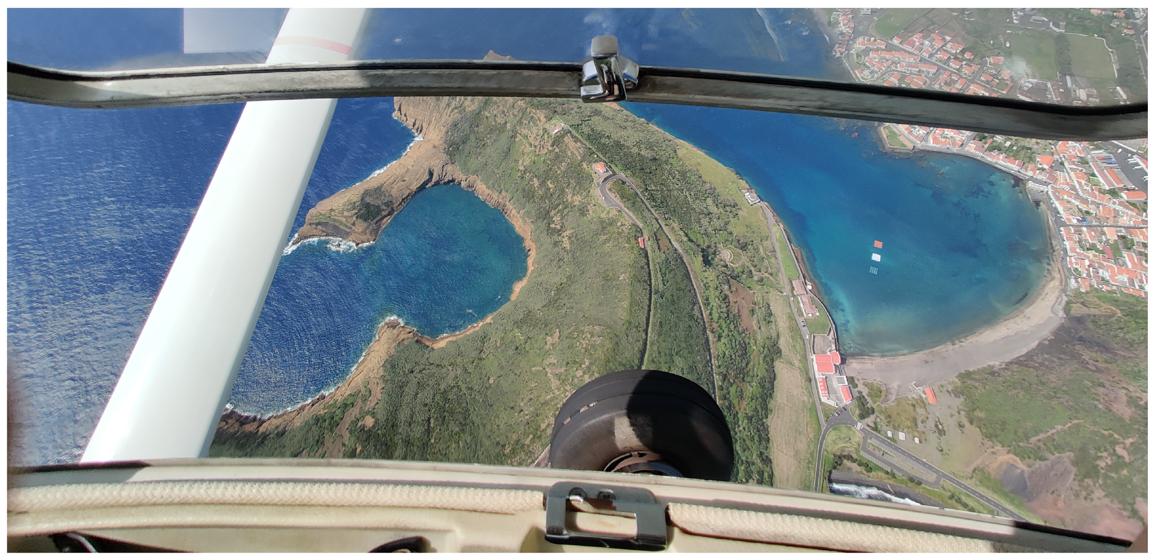
One of the goals of this campaign was also to assess Sentinel-2 (S2) satellite capability to detect marine litter and compare the results using satellite and airborne data. Due to the S2 spatial resolution, there was the need of having 10 × 10 metre artificial targets to be visible by the satellite. For this purpose, we used three different artificial targets, which were composed of distinct types of plastic: low-density polyethylene orange plastic (used oyster spat collectors), white plastic film, and ropes. Figure 6 shows the targets already in the water. In addition to the flybys over the targets, the dataset also holds information about other materials and objects present in the data, namely: water, concrete pier, trees, and boats. These data will also be used in our algorithm to train the ZSL method.

Figure 6.
Image acquired from the aircraft during a flight with the artificial targets placed in the water.
Due to the type of hyperspectral image acquisition system (pushbroom), the dataset was collected during a single flight and contains information about other artefacts that are difficult to manually label such as streets with moving cars and houses. Therefore, the solution used was to divide the dataset into flybys over the classes that can be manually labelled, such as water, orange target, white target, rope target, concrete pier, trees, and boats.
Table 1 shows the description of all the data present in the dataset and provides an example of each class.

Table 1.
Classes used for the ZSL algorithm, and main characteristics, e.g., description, known and unknown information, image and number of pixels.
Having defined the classes for the ZSL implementation, one needs to divide them into the set of known and unknown classes. Since our objective was to detect marine litter (plastic), we choose two of the artificial plastic targets as unknown classes: class 1—orange plastic target and class 3—ropes target.
We then started the training procedure, where adjustments had to be performed to overcome the limitations of the training data, namely:
- Class imbalance: As shown in Table 1, the number of pixels for each class is different. To minimise the probability of overfitting during training, we use the lower number of pixels as a reference to randomly select samples from the other classes;
- Feature normalisation: The hyperspectral data acquisition is affected by the variability of atmospheric conditions, mainly direct sunlight. To minimise this effect, there is the need to perform the data normalisation in order to normalise the feature data to unit variance.
In addition to the aforementioned pre-processing techniques, we also had to take into account some items concerning each of the known and unknown classes, such as:
- Due to the flight altitude, some of the classes will have small (resolution) in the datasets. In addition to this, there are classes with artefacts in the middle due to their physical characteristics and construction. This happens in class 1, orange target, and class 3, rope target. The first, given the physical design of the multiple components (used oyster spat collectors) and their orientation, can accumulate more water, while the second (rope target) has more gaps in the middle of the target. Additionally, this target also uses two different rope targets with variable flutuability.
- The water contains points with high exposure due to the wave effects and the camera adjustment.
- The concrete pier also contains rocks.
- It is necessary to take into account that in class 6, boats have different hulls, and there are artefacts inside the boat that also have different materials. However, the flight altitude combined with the cameras spatial resolution does not allow a better distinction to facilitate the manual labelling process.
Another influential aspect is the camera exposure time. During the data collection, the exposure time was set to acquire the plastic targets in the best manner possible. Therefore, it can lead to overexposed zones that hold other classes and negatively influences the results.
4. Results
In this section, we will display the ZSL results for marine litter detection and classification. In this experiment, the algorithm was trained using seven classes in total: class 0, 2, 4, 5, and 6 are the known classes, while the unknown classes (two of the plastic targets) were classes 1 and 3. Since one the main objectives is to understand if the method can detect new plastic types that are not yet determined (unknown), we prefer to train with only one known plastic type. However, this will negatively influence the results due to the intrinsic physical characteristics of the plastic materials.
After performing the selection, we divided the dataset into training, validation, and test data. To promote the balance between the data, the number of points for each class used for training was 5023, and the number of pixels present in the class with fewer samples, class 6—boats, was selected randomly. The data were then divided using 70% to train, 10% for validation, and all the remaining data to test, including data outside the first division.
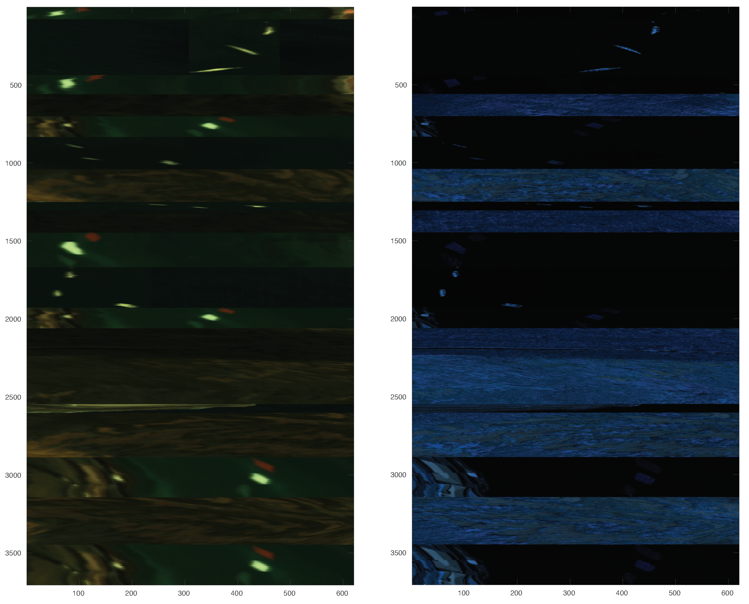
Figure 7 shows the reconstructed image of the dataset for both SPECIM FX10E (400–1000 nm) and HySpex Mjolnir S-620 (970–2500 nm) systems, respectively, where it is possible to observe that there are multiple flybys over all the targets.
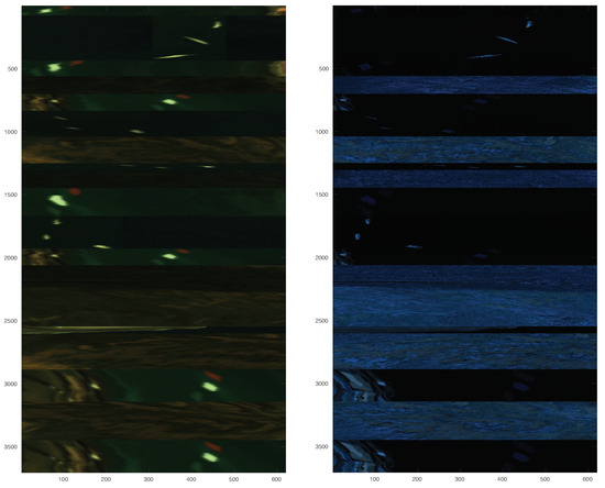
Figure 7.
Reconstructed image for each hyperspectral camera used. Left image shows the Specim FX-10e data, while right image shows the HySpex Mjolnir S-620 data.
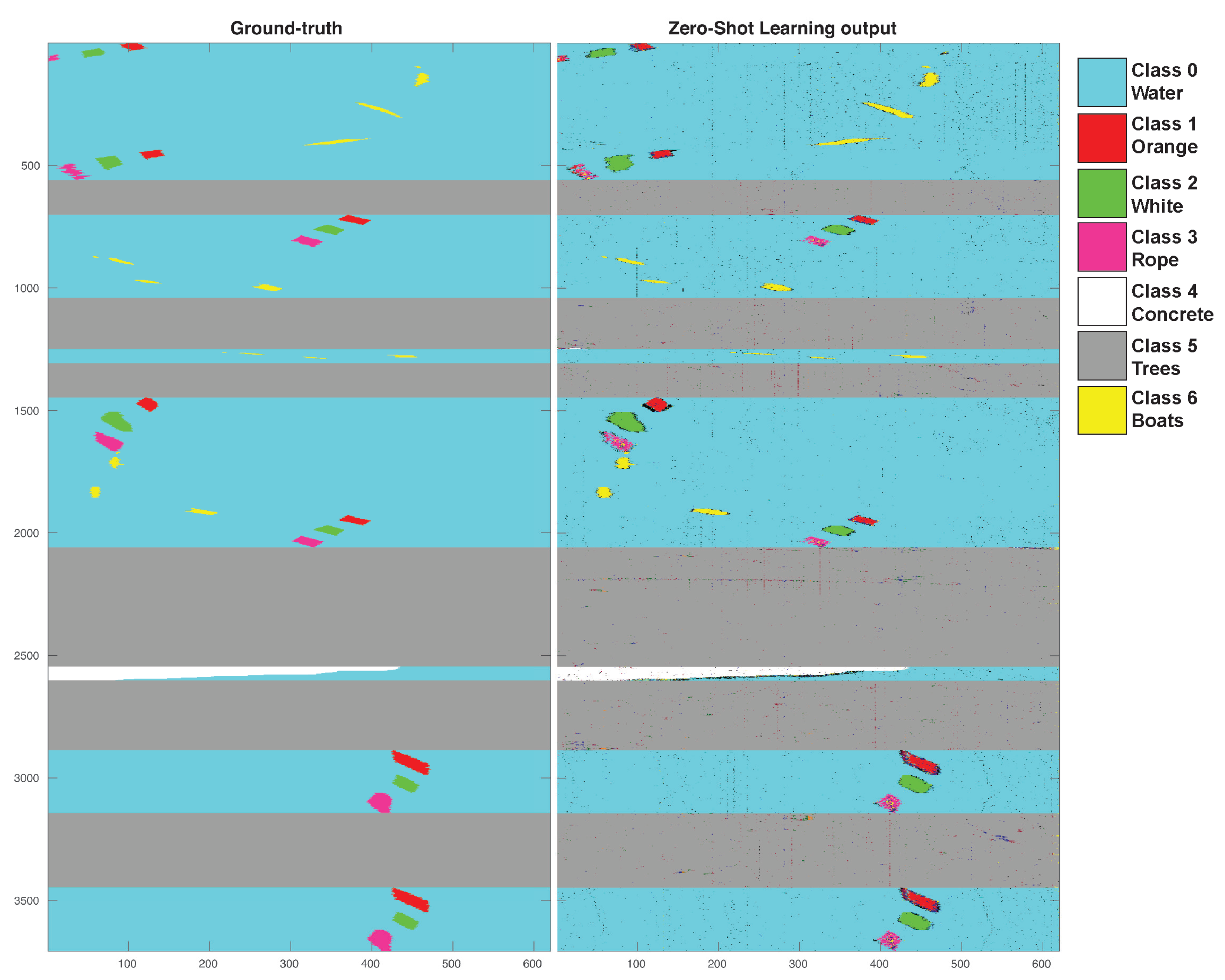
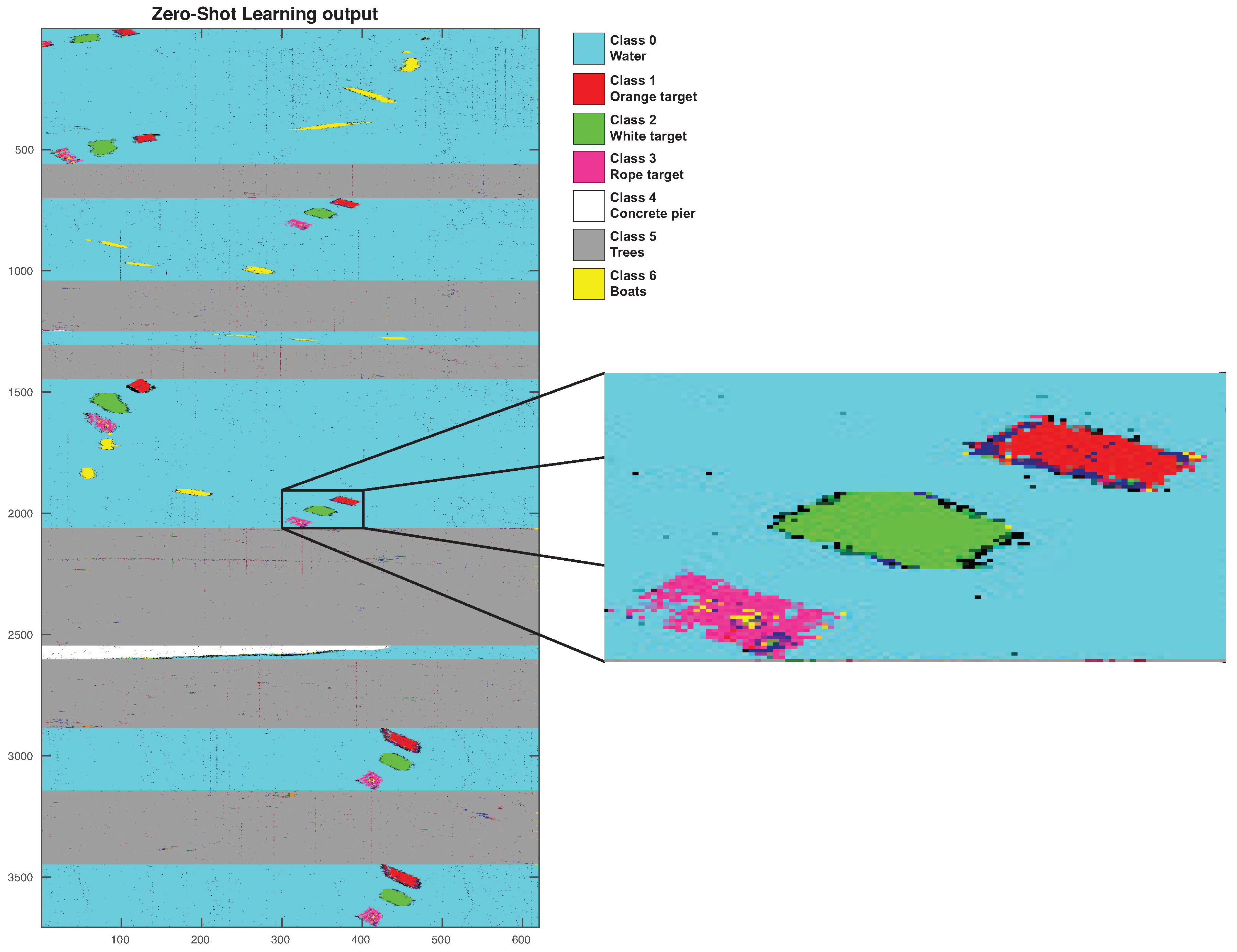
Figure 8 shows the manually annotated ground truth image on the left-hand side, while the right-hand side of the figure contains the ZSL results. Both images follow the same colour scheme to identify the different classes. There are some pixel outliers that represent four more classes, which are represented in orange, light pink, light grey and dark green. The colour scheme for each class is identified in the first column of Table 1. Figure 9 shows a zoom-enhanced version of one of the artificial target detections. It is possible to observe the two unknown classes (class 1—orange target, red colour, and class 3—rope target, pink colour) and some of the outliers around the edges.

Figure 8.
Left image holds the ground truth while the right image shows the zero-shot learning results.

Figure 9.
Zero-shot learning results zooming on one of the artificial target’s detections (including the two unknown classes (class 1, identified with the colour red, and class 3, identified with the colour pink).
Concerning the experimental setup, the tests were performed in a workstation with an Intel Core i7-8700k @ 3.70 GHz CPU, 32 GB RAM memory and one GeForce RTX 2080 Super 8 GB. The training stage took approximately 1052.71 s, while the prediction took approximately 243.44 s to finish.
To perform a comparison between the novel ZSL approach and already established state-of-the-art approaches, we compared the results (for the unknown samples) obtained by the ZSL with our previous work Random Forest (RF) and Support Vector Machines (SVM) implementation [5], and CNN-3D [6] for the same experimental data setup. We expect the ZSL performance metrics to be below that of the other methods, as in the ZSL RGB approaches, since the other methods are based on supervised approaches with all known samples. However, it is important to understand the order of magnitude the ZSL can perform and if it is viable to use this semi-supervised or even unsupervised approaches in remote airborne hyperspectral imaging systems for marine litter detection.
Table 2 shows the zero-shot learning results, while Table 3 shows a comparison between these and the previous results, obtained and presented in [5,6].

Table 2.
Zero-Shot Learning Results.

Table 3.
Results comparison using RF, SVM, CNN and ZSL methods.
5. Discussion
In this section, we will discuss the results obtained by the ZSL method, particularly focusing on the ability to detect the unknown classes. We also compare and discuss the results obtained with our previous implementations (RF, SVM and CNN3D). Table 2 depicts each class’s precision, recall, f1-score, the accuracy of each class, and overall accuracy (OA). One can observe that unknown classes 1 and 3 both have recall values over 57%, which means that the true positive pixels were higher than 57% of the total samples in both cases. In terms of precision, class 1 has more than 66% while class 3 has more than 56%.
Given the average flight altitude, 600 m, is it difficult to manually annotate the pixels as being purely belonging to a single class. This makes it difficult to assure that each pixel in the targets belonging to classes 1, 2, and 3 is not contaminated by water. In addition, the targets’ morphology and their constituents also make this task difficult. The targets had 10 × 10 m, composed of four squares, each one with 2.5 × 2.5 m, each target filled with the corresponding material. However, for example, in the case of class 3—ropes, the filling is not uniform due to the water effects, creating areas where the target is submerged, which is a phenomena that also occurs with class 1—orange target.
Regarding class 6—boats, precision is over 58%, and the recall is over 99%, which indicates a high number of true positives (over 99% of the pixels are correctly identified as class 6). However, it also shows some false positives. In this case, the false positives are present in the water, which raises the issue of the ground truth annotation: due to the resolution, it is impossible to understand what is inside the boats. These were not placed in the water, especially for dataset purposes, so we do not have any control over what is inside them.
Figure 9 shows a zoom for one of the artificial target’s ZSL results. As observed, the class 3—rope target, represented by the pink points, exhibits some points marked as class 6—boats (yellow). This shows that some of the boats can probably have ropes inside them. However, the spatial resolution makes it impossible to understand what is inside the boat. The pixel may not be pure (representing only one type of material) and instead be a combination of different materials inside the boat. It is also possible to observe some points marked as class 6—boats (yellow) in the limits of the artificial targets, which is probably due to the water bottles used to help them float. Another issue is the camera configuration and the set of the camera gain that is configured to acquire the artificial target data. Effects such as sun reflections can result in over-exposure pixels, mainly on pixels that do not represent the classes that the cameras were configured to acquire. This is especially noticeable in the waves of the water, which have several over-exposure pixels.
Analysing the left image in Figure 8, it is possible to observe the presence of different classes that do not belong to the ones identified by the ground truth near the concrete pier (class 5, color grey). These are located in the rocks of the pier, which is most likely due to the foam created with the ocean motion due to oil residues, among others. However, it is impossible to identify this on the ground truth due to the camera’s spatial resolution. This is also visible in Figure 9, in the contour of the orange and white artificial targets, and it can also be due to the foam that forms next to these targets due to the water ripple. This is not so visible in the rope target due to its characteristics: the ropes absorb much more water and offers less resistance to the water passage due to their shape.
Despite being a challenging dataset, due to the impossibility of controlling what is in the data that do not belong to the artificial targets, the ZSL algorithm acquired knowledge about the known classes and was able to detect and classify the unknown classes to a reasonable extent.
Although this approach presents interesting results, using other algorithms to extract more meaningful information from the spectra can be an interesting solution. One approach that could extract more information about the characteristics of the plastics is the band selection algorithm, which will not project the data to another space, such as the method used for dimensionality reduction in this work (PCA algorithm).
Using spatial information combined with spectral one can be an interesting solution. However, this dataset was built from multiple flybys over points of interest (over the different classes: artificial targets, water, trees and boats), since the full dataset contained several areas whose ground truth was impossible to perform (roads with cars and people moving, for example), so there was a need to discard these data. Given this, the spatial information was compromised by this dataset construction and could negatively influence the algorithm to learn some spatial representation that is not true. In addition to this, there is the fact that the artificial targets used for proof-of-concept are a perfectly square shape, which will not happen in a real scenario. The deformations suffered by the marine litter during their life are mainly due to sun exposure and water erosion and hitting other artefacts such as more marine litter and rocks, among others. These deformations will change the marine litter shape but without affecting the spectral information.
In Table 3, it is possible to compare our state-of-the art results and the zero-shot learning approach. Some remarks should be addressed before analysing this table:
- Random Forest (RF), Support Vector Machine (SVM) and the Convolutional Neural Network 3D (CNN3D) were all implemented using only four classes:
- –
- Class 0: For the RF and SVM algorithm, it represents the water and land (houses, trees, streets, cars and other materials) to train the algorithms to learn the characteristics of the non-marine litter pixels. In the case of the CNN3D algorithm, it represents the water;
- –
- Class 1: orange target;
- –
- Class 2: white target;
- –
- Class 3: rope target.
- RF, SVM, and ZSL approaches use the F-BUMA data, while the CNN3D resorts to the drone data, using the same artificial targets and in the same test site. Due to the lack of resolution of the F-BUMA data, the results of the CNN3D were unsatisfactory due to the lack of distinct spatial features. Although the drone data have much more spatial information, as can be observed in [6], it does not contain data from any other class besides the artificial targets and the water, which was not enough for the ZSL algorithm. It would be possible to use RF and SVM with drone data. However, the algorithms will not benefit from the spatial information, and therefore, no novelty will be added to the results obtained with the F-BUMA data;
- The datasets used for RF, SVM and CNN3D algorithms were organised by flyby over the artificial targets, giving each flyby its results. In the case of the SVM and RF, Table 3 only presents the results for a single flybys (there were six flybys in total), while in the case of the CNN3D, all the results are presented.
Due to the difference in the number of classes, it is impossible to compare the accuracy directly. However, it is possible to analyse the precision, recall and F1-score for the artificial targets classes (classes 1, 2 and 3). However, given that F1-score is a combination of the precision and recall values, the analysis will focus on the precision and recall results. Observing the results for class 1, orange target, in terms of precision, the values are similar. In the case of the ZSL approach, this algorithm was not trained with data from this class and can still obtain comparable results in terms of precision compared to the other three algorithms. When comparing the recall values, it is possible to observe that both the RF and SVM results are lower than the ZSL approach, and when comparing ZSL and CNN3D, the results are similar. Class 2, white target, a known class for the ZSL algorithm, i.e., the model was trained with data from this class, also presents similar results for all the approaches. SVM shows lower performance, while CNN3D display better results. However, ZSL performs better than the RF algorithm in terms of precision and recall. The last comparable class is the number 3, rope target, which is the most challenging for all the methods due to their characteristics. This is evident in the results presented for all the algorithms, with CNN3D performing slightly better. ZSL overcomes both RF and SVM approaches, even considering that this was an unknown class whose data were hidden during the training phase of the ZSL model.
Overall, the ZSL algorithm shows potential to detect unknown marine litter, i.e., plastic samples using a hyperspectral imaging system installed in an aircraft at approximately 600 m altitude, with precision values over 56% for all the classes, including the two unknown classes, which are not used to train the model. This is in line with the results obtained by ZSL methods using only visible images and therefore shows that ZSL methods can also have potential applications in hyperspectral imaging data.
6. Conclusions
Novel research aims to provide solutions to detect and analyse marine litter, to understand its origin and the best way to decrease its presence in our oceans. Hyperspectral imaging is one possible solutions due to the amount of relevant information collected from a scene. However, most detection algorithms are based on supervised machine learning techniques, which implies using labelled data for all classes. This is a difficult task in the marine litter field due to the massive amount of different artefacts and the changes they suffer from erosion and sunlight.
Our work focuses on the development of a zero-shot learning method for remote hyperspectral imaging data on detecting and classifying marine litter. This novel algorithm detects unknown classes, i.e., classes not seen by the model during the training stage, which is useful to decrease the number of samples needed to train the model and allows the classification of samples without previous information.
We used an approach divided into four different components: feature extractor, classifier, decoder, and discriminator, where the first three components are used to build a semantic space for the spectra. We were able to train a model with only five known classes capable of recognising two new types of plastic. All metrics for both unknown classes are over 56%, which proves the algorithm’s capability to detect and classify new classes that were never seen during training. The overall accuracy for all classes is over 98%, showing promising results for this type of classification. All the results were evaluated using a previously acquired dataset [5].
Zero-shot learning approaches show an advantage of classifying samples for which the model was not trained and did not have access during the training stage. Although these methods do not achieve the same results as the state-of-the-art classification algorithms for hyperspectral imaging, they reduce the training data, and it can detect and classify classes that were never seen by the algorithm.
In future work, we would like to focus on applying this ZSL algorithm in real time, to perform regular flights and identify marine litter concentrations near coastal areas, offshore aquaculture farms, and remote locations that are not covered by satellites. The application of this algorithm to satellite data would also be interesting. Another question we would like to focus our attention is on is the application of band selection methods to extract more meaningful information about the plastics that allow a more robust classification even of the unknown classes.
Author Contributions
Conceptualization, H.S. and E.S.; methodology, H.S. and S.F.; software, S.F.; validation, S.F.; formal analysis, H.S.; investigation, S.F.; resources, E.S. and H.S.; data curation, S.F.; writing—original draft preparation, S.F.; writing—review and editing, H.S.; visualization, S.F.; supervision, H.S.; project administration, E.S.; funding acquisition, E.S. All authors have read and agreed to the published version of the manuscript.
Funding
This work is financed by National Funds through the Portuguese funding agency, FCT—Fundação para a Ciência e Tecnologia, within project UIDB/50014/2020, by the European Space Agency (ESA) within the contract 4000129488/19/NL/BJ/ig, by the European Commission under the H2020 EU Framework Programme for Research and Innovation within project H2020-WIDESPREAD-2018-03, 857339 and by National Funds through the FCT-Fundação para a Ciência e Tecnologia under grant SFRH/BD/139103/2018 and COVID/BD/152190/2021.
Acknowledgments
The authors would like to thank ACTV (Aeroclube Torres de Vedras) for providing the F-BUMA airplane, and Ocean Science Institute–OKEANOS Universidade dos Açores team for providing the targets and personal help during the experiments. Additionally, we thank the Observatório do Mar dos Açores (OMA) for accessing their facilities during the operation.
Conflicts of Interest
The authors declare no conflict of interest.
References
- Ciappa, A. Marine Litter Detection by Sentinel-2: A Case Study in North Adriatic (Summer 2020). Remote Sens. 2022, 14, 2409. [Google Scholar] [CrossRef]
- Maximenko, N.; Corradi, P.; Law, K.L.; Van Sebille, E.; Garaba, S.P.; Lampitt, R.S.; Galgani, F.E.A. Toward the Integrated Marine Debris Observing System. Front. Mar. Sci. 2019. [Google Scholar] [CrossRef]
- Topouzelis, K.; Papageorgiou, D.; Suaria, G.; Aliani, S. Floating marine litter detection algorithms and techniques using optical remote sensing data: A review. Mar. Pollut. Bull. 2021, 170, 112675. [Google Scholar] [CrossRef] [PubMed]
- Fulton, M.; Hong, J.; Islam, M.J.; Sattar, J. Robotic Detection of Marine Litter Using Deep Visual Detection Models. arXiv 2019, arXiv:1804.01079. [Google Scholar] [CrossRef]
- Freitas, S.; Silva, H.; Silva, E. Remote Hyperspectral Imaging Acquisition and Characterization for Marine Litter Detection. Remote Sens. 2021, 13, 2536. [Google Scholar] [CrossRef]
- Freitas, S.; Silva, H.; Almeida, C.; Viegas, D.; Amaral, A.; Santos, T.; Dias, A.; Jorge, P.A.S.; Pham, C.K.; Moutinho, J.; et al. Hyperspectral Imaging System for Marine Litter Detection. In OCEANS 2021: San Diego—Porto; IEEE: New York, NY, USA, 2021; pp. 1–6. [Google Scholar] [CrossRef]
- Martínez-Vicente, V.; Clark, J.R.; Corradi, P.; Aliani, S.; Arias, M.; Bochow, M.; Bonnery, G.; Cole, M.; Cózar, A.; Donnelly, R.; et al. Measuring Marine Plastic Debris from Space: Initial Assessment of Observation Requirements. Remote Sens. 2019, 11, 2443. [Google Scholar] [CrossRef]
- Kremezi, M.; Kristollari, V.; Karathanassi, V.; Topouzelis, K.; Kolokoussis, P.; Taggio, N.; Aiello, A.; Ceriola, G.; Barbone, E.; Corradi, P. Pansharpening PRISMA Data for Marine Plastic Litter Detection Using Plastic Indexes. IEEE Access 2021, 9, 61955–61971. [Google Scholar] [CrossRef]
- Topouzelis, K.; Papageorgiou, D.; Karagaitanakis, A.; Papakonstantinou, A.; Arias Ballesteros, M. Remote Sensing of Sea Surface Artificial Floating Plastic Targets with Sentinel-2 and Unmanned Aerial Systems (Plastic Litter Project 2019). Remote Sens. 2020, 12, 2013. [Google Scholar] [CrossRef]
- Wolf, M.; van den Berg, K.; Garaba, S.P.; Gnann, N.; Sattler, K.; Stahl, F.; Zielinski, O. Machine learning for aquatic plastic litter detection, classification and quantification (APLASTIC-Q). Environ. Res. Lett. 2020, 15, 114042. [Google Scholar] [CrossRef]
- Park, Y.J.; Garaba, S.P.; Sainte-Rose, B. Detecting the Great Pacific Garbage Patch floating plastic litter using WorldView-3 satellite imagery. Opt. Express 2021, 29, 35288–35298. [Google Scholar] [CrossRef]
- Kumar, N.; Berg, A.C.; Belhumeur, P.N.; Nayar, S.K. Attribute and Simile Classifiers for Face Verification. In Proceedings of the IEEE International Conference on Computer Vision (ICCV), Kyoto, Japan, 29 September–2 October 2009. [Google Scholar]
- Lampert, C.H.; Nickisch, H.; Harmeling, S. Attribute-Based Classification for Zero-Shot Visual Object Categorization. IEEE Trans. Pattern Anal. Mach. Intell. 2014, 36, 453–465. [Google Scholar] [CrossRef] [PubMed]
- Xu, B.; Fu, Y.; Jiang, Y.; Li, B.; Sigal, L. Video Emotion Recognition with Transferred Deep Feature Encodings. In Proceedings of the 2016 ACM on International Conference on Multimedia Retrieval, New York, NY, USA, 6–9 June 2016. [Google Scholar]
- Fu, Y.; Hospedales, T.M.; Xiang, T.; Gong, S. Attribute Learning for Understanding Unstructured Social Activity. In Computer Vision—ECCV 2012. ECCV 2012. Lecture Notes in Computer Science; Springer: Berlin/Heidelberg, Germany, 2012; Volume 7575. [Google Scholar] [CrossRef]
- Liu, J.; Kuipers, B.; Savarese, S. Recognizing Human Actions by Attributes. In Proceedings of the IEEE Conference on Computer Vision and Pattern Recognition (CVPR), Colorado Springs, CO, USA, 20–25 June 2011; pp. 3337–3344. [Google Scholar]
- Fu, Y.; Hospedales, T.M.; Xiang, T.; Gong, S. Learning Multimodal Latent Attributes. IEEE Trans. Pattern Anal. Mach. Intell. 2014, 36, 303–316. [Google Scholar] [CrossRef] [PubMed]
- Blitzer, J.; Foster, D.P.; Kakade, S.M. Zero-Shot Domain Adaptation: A Multi-View Approach. Technical Report TTI-TR-2009-1. 2009. Available online: https://www.ttic.edu/technical_reports/ttic-tr-2009-1.pdf (accessed on 29 July 2022).
- Long, Y.; Liu, L.; Shao, L. Attribute embedding with visual-semantic ambiguity removal for zero-shot learning. In Proceedings of the British Machine Vision Conference 2016, York, UK, 19–22 September 2016. [Google Scholar]
- Zhang, Z.; Saligrama, V. Zero-shot learning via joint latent similarity embedding. In Proceedings of the IEEE Conference on Computer Vision and Pattern Recognition (CVPR), Las Vegas, NV, USA, 27–30 June 2016; pp. 6034–6042. [Google Scholar]
- Xian, Y.; Akata, Z.; Sharma, G.; Nguyen, Q.; Hein, M.; Schiele, B. Latent embeddings for zero-shot classification. In Proceedings of the IEEE Conference on Computer Vision and Pattern Recognition, Las Vegas, NV, USA, 27–30 June 2016; pp. 69–77. [Google Scholar]
- Norouzi, M.; Mikolov, T.; Bengio, S.; Singer, Y.; Shlens, J.; Frome, A.; Corrado, G.; Dean, J. Zero-Shot Learning by Convex Combination of Semantic Embeddings. arXiv 2013, arXiv:1312.5650. [Google Scholar]
- Zhang, Z.; Saligrama, V. Zero-shot learning via semantic similarity embedding. In Proceedings of the IEEE International Conference on Computer Vision, Santiago, Chile, 7–13 December 2015; pp. 4166–4174. [Google Scholar]
- Akata, Z.; Perronnin, F.; Harchaoui, Z.; Schmid, C. Label-Embedding for Image Classification. IEEE Trans. Pattern Anal. Mach. Intell. 2016, 38, 1425–1438. [Google Scholar] [CrossRef]
- Frome, A.; Corrado, G.; Shlens, J.; Bengio, S.; Dean, J.; Ranzato, M.; Mikolov, T. DeViSE: A Deep Visual-Semantic Embedding Model. In Proceedings of the Advances in Neural Information Processing Systems 26 (NIPS 2013), Lake Tahoe, NV, USA, 5–10 December 2013; pp. 2121–2129. [Google Scholar]
- Paredes, B.R.; Torr, P.H.S. An Embarrassingly Simple Approach to Zero-shot Learning. In Proceedings of the 32nd International Conference on International Conference on Machine Learning—Volume 37. JMLR.org, Lille, France, 7–9 July 2015; pp. 2152–2161. [Google Scholar]
- Changpinyo, S.; Chao, W.; Gong, B.; Sha, F. Synthesized Classifiers for Zero-Shot Learning. In Proceedings of the IEEE Conference on Computer Vision and Pattern Recognition (CVPR), Las Vegas, NV, USA, 27–30 June 2016. [Google Scholar]
- Zhang, Z.; Saligrama, V. Learning Joint Feature Adaptation for Zero-Shot Recognition. arXiv 2016, arXiv:1611.07593. [Google Scholar]
- Kodirov, E.; Xiang, T.; Fu, Z.; Gong, S. Unsupervised domain adaptation for zero-shot learning. In Proceedings of the IEEE International Conference on Computer Vision, Santiago, Chile, 7–13 December 2015; pp. 2452–2460. [Google Scholar]
- Zhang, Z.; Saligrama, V. Zero-shot recognition via structured prediction. In Proceedings of the European Conference on Computer Vision (ECCV), Amsterdam, The Netherlands, 11–14 October 2016; pp. 533–548. [Google Scholar]
- Fu, Y.; Hospedales, T.M.; Xiang, T.; Fu, Z.; Gong, S. Transductive multi-view embedding for zero-shot recognition and annotation. In Proceedings of the European Conference on Computer Vision (ECCV), Zurich, Switzerland, 6–12 September 2014; pp. 584–599. [Google Scholar]
- Guo, Y.; Ding, G.; Jin, X.; Wang, J. Transductive Zero-shot Recognition via Shared Model Space Learning. In Proceedings of the Thirtieth AAAI Conference on Artificial Intelligence, Phoenix, AZ, USA, 12–17 February 2016; pp. 3494–3500. [Google Scholar]
- Song, J.; Shen, C.; Yang, Y.; Liu, Y.; Song, M. Transductive Unbiased Embedding for Zero-Shot Learning. In Proceedings of the 2018 IEEE/CVF Conference on Computer Vision and Pattern Recognition (CVPR), Salt Lake City, UT, USA, 18–23 June 2018. [Google Scholar]
- Salakhutdinov, R.; Tenenbaum, J.B.; Torralba, A. Learning with Hierarchical-Deep Models. IEEE Trans. Pattern Anal. Mach. Intell. 2013, 35, 1958–1971. [Google Scholar] [CrossRef]
- Mensink, T.; Gavves, E.; Snoek, C.G.M. COSTA: Co-Occurrence Statistics for Zero-Shot Classification. In Proceedings of the IEEE Conference on Computer Vision and Pattern Recognition (CVPR), Columbus, OH, USA, 23–28 June 2014; pp. 2441–2448. [Google Scholar] [CrossRef]
- Chao, W.; Changpinyo, S.; Gong, B.; Sha, F. An Empirical Study and Analysis of Generalized Zero-Shot Learning for Object Recognition in the Wild. In Proceedings of the Computer Vision–ECCV 2016, Amsterdam, The Netherlands, 11–14 October 2016; pp. 52–68. [Google Scholar]
- Felix, R.; Kumar, B.G.V.; Reid, I.; Carneiro, G. Multi-modal Cycle-consistent Generalized Zero-Shot Learning. In Proceedings of the European Conference on Computer Vision (ECCV), Munich, Germany, 8–14 September 2018. [Google Scholar]
- Verma, V.K.; Arora, G.; Mishra, A.; Rai, P. Generalized Zero-Shot Learning via Synthesized Examples. In Proceedings of the IEEE Conference on Computer Vision and Pattern Recognition (CVPR), Salt Lake City, UT, USA, 18–23 June 2018. [Google Scholar]
- Qu, Y.; Baghbaderani, R.K.; Qi, H. Few-Shot Hyperspectral Image Classification Through Multitask Transfer Learning. In Proceedings of the 10th Workshop on Hyperspectral Imaging and Signal Processing: Evolution in Remote Sensing (WHISPERS), Amsterdam, The Netherlands, 24–26 September 2019; pp. 1–5. [Google Scholar] [CrossRef]
- Liu, S.; Shi, Q.; Zhang, L. Few-Shot Hyperspectral Image Classification With Unknown Classes Using Multitask Deep Learning. IEEE Trans. Geosci. Remote Sens. 2021, 59, 5085–5102. [Google Scholar] [CrossRef]
- Wang, Y.; Liu, M.; Yang, Y.; Li, Z.; Du, Q.; Chen, Y.; Li, F.; Yang, H. Heterogeneous Few-Shot Learning for Hyperspectral Image Classification. IEEE Geosci. Remote Sens. Lett. 2022, 19, 1–5. [Google Scholar] [CrossRef]
- Li, Z.; Liu, M.; Chen, Y.; Xu, Y.; Li, W.; Du, Q. Deep Cross-Domain Few-Shot Learning for Hyperspectral Image Classification. IEEE Trans. Geosci. Remote Sens. 2022, 60, 1–18. [Google Scholar] [CrossRef]
- Tong, X.; Yin, J.; Han, B.; Qv, H. Few-Shot Learning With Attention-Weighted Graph Convolutional Networks For Hyperspectral Image Classification. In Proceedings of the IEEE International Conference on Image Processing (ICIP), Abu Dhabi, United Arab Emirates, 25–28 October 2020; pp. 1686–1690. [Google Scholar] [CrossRef]
- Ding, C.; Li, Y.; Wen, Y.; Zheng, M.; Zhang, L.; Wei, W.; Zhang, Y. Boosting Few-Shot Hyperspectral Image Classification Using Pseudo-Label Learning. Remote Sens. 2021, 13, 3539. [Google Scholar] [CrossRef]
- Pal, D.; Bundele, V.; Sharma, R.; Banerjee, B.; Jeppu, Y. Few-Shot Open-Set Recognition of Hyperspectral Images with Outlier Calibration Network. In Proceedings of the IEEE/CVF Winter Conference on Applications of Computer Vision (WACV), Waikoloa, HI, USA, 3–8 January 2022; pp. 2091–2100. [Google Scholar] [CrossRef]
- Dong, Y.; Jiang, X.; Zhou, H.; Lin, Y.; Shi, Q. SR2CNN: Zero-Shot Learning for Signal Recognition. arXiv 2020, arXiv:2004.04892. [Google Scholar] [CrossRef]
- Rodarmel, C.; Shan, J. Principal Component Analysis for Hyperspectral Image Classification. Surv. Land Inf. Syst. 2002, 62, 115–122. [Google Scholar]
- Woo, S.; Park, J.; Lee, J.Y.; Kweon, I.S. CBAM: Convolutional Block Attention Module. arXiv 2018, arXiv:1807.06521. [Google Scholar] [CrossRef]
- Wen, Y.; Zhang, K.; Li, Z.; Qiao, Y. A Discriminative Feature Learning Approach for Deep Face Recognition. In Computer Vision—ECCV 2016; Leibe, B., Matas, J., Sebe, N., Welling, M., Eds.; Springer International Publishing: Cham, Switzerland, 2016; pp. 499–515. [Google Scholar]
Publisher’s Note: MDPI stays neutral with regard to jurisdictional claims in published maps and institutional affiliations. |
© 2022 by the authors. Licensee MDPI, Basel, Switzerland. This article is an open access article distributed under the terms and conditions of the Creative Commons Attribution (CC BY) license (https://creativecommons.org/licenses/by/4.0/).

