Convolutional Neural Networks for Agricultural Land Use Classification from Sentinel-2 Image Time Series

Abstract

Land use classification (LUC) is the process of providing information on land cover and the types of human activity involved in land use. In this study, we perform agricultural LUC using sequences of multispectral reflectance Sentinel-2 images taken in 2018. LUC can be carried out using machine or deep learning techniques. Some existing models process data at the pixel level, performing LUC successfully with a reduced number of images. Part of the pixel information corresponds to multispectral temporal patterns that, despite not being especially complex, might remain undetected by models such as random forests or multilayer perceptrons. Thus, we propose to arrange pixel information as 2D yearly fingerprints so as to render such patterns explicit and make use of a CNN to model and capture them. The results show that our proposal reaches a 91% weighted accuracy in classifying pixels among 19 classes, outperforming random forest by 8%, or a specifically tuned multilayer perceptron by 4%. Furthermore, models were also used to perform a ternary classification in order to detect irrigated fields, reaching a 97% global accuracy. We can conclude that this is a promising operational tool for monitoring crops and water use over large areas.

1. Introduction

Agriculture is a key sector from an economic, social, and environmental point of view. Because of its high demand for water and nutrient inputs for increasing the yield, agriculture places high pressure on the surface and groundwater resources. This is an important issue for governments, policymakers, farmers, and other organizations, as estimations predict that, in order to cover the food demand by 2050, a 60% increment production will be needed [1]. Policies from the international to local scale are facing the challenge of providing natural resource managers with the tools required for the sustainability of food supply sectors and resilience to climate change [2,3,4]. In particular, the European and national authorities estimate the number of subsidies on the farm scale by considering farmers’ reports about their practices for crop management, such as water use, fertilizers, and energy, which are properly supervised by experts who help to encourage sustainable use. In this scenario, precise crop and land use classification (LUC) are necessary for assisting in the management of sustainable natural resources [5] and also facing the consequences of climate change [6]. LUC is the basic information required for the sustainable use of land, water, energy management, and the environment [7]. Nevertheless, even gathering information about the harvested crops and their management has a high cost when it requires fieldwork.

Remote sensing is one of the main sources of information in this context. It can be applied to large areas and provides classification maps at a lower cost. The plot scale in remote sensing is limited by the pixel size of the images acquired by the sensors. However, due to the increase in both the spatiotemporal resolution of the data and processing power, improvements are becoming important in recent years [8]. Hence, Sentinel and Landsat constellations provide data to monitor plots below 0.3 ha, which is adequate for most agricultural areas [9].

Traditionally, the generation of an LUC map has consisted of the examination of multi-spectral and temporal sensor data at single positions and their surrounding areas. Therefore, a long time series of images at a high temporal frequency provides data that can be used to identify vegetation types with a high confidence level [10]. Those algorithms are based on biophysical variables that vary over time according to the specific phenology of each crop, the agronomic management, and the environmental conditions. Regarding the importance of such temporal signatures, sensors with a high temporal resolution, such as MODIS, have been used for this purpose despite their low resolution (from 250 m to 1 km depending on the data) [11,12], providing good results, since they gather the sequential information of a specific location over time [13]. The scenario is even more favorable nowadays, as there is an availability of multi-spectral remote sensing data of a relatively fine resolution (from 10 m to 60 m), provided by the Sentinel 2 constellation with a reasonable revisit frequency of 5 days [14].

The first generation of procedures for LUC maps relied on experts who built models based on indexes calculated from the bands of the satellite images, such as the temporal evolution of NDVI, which is calculated as the near-infrared (NIR) minus red reflectance, divided by the near-infrared plus red reflectance [15]. NDVI can be used to identify the land use of a single point with a reasonable computational cost [16]. The attempts and the progress in efforts to automate the process of land use classification are moving towards the use of machine learning, an area of artificial intelligence. Machine learning models use features to identify patterns in datasets. When such patterns involve a target variable, these can be used to perform tasks such as classification. Gilabert et al. showed that temporal information can be extracted from the spectral bands [17]. Experts manually fine-tuned the rules of those interpretable models based on simpler variables, according to their expertise regarding how features determine the type of crop and the knowledge about a concrete region [18]. Foerster et al. [13] and Hao et al. [19] proposed solutions based on NDVI that use decision trees and random forest models, respectively, with a pixel-based approach. J. Inglada et al. tested random forests and support vector machines in crop classification using feature extractions, such as derived indices [9]. Immitzer et al. proved that the most important bands of the Sentinel-2 images are the blue, red-edge, and shortwave infrared for crop classification in a study applying a random forest model [20]. Additionally, authors such as Hao et al. indicated that it is possible to merge datasets with a similar spatial resolution in order to enrich the time series [21]. Zhou et al. reported that optimizing the required number of images, resulting in a reduction in the time series length, had almost no impact on the accuracy of the classification [22].

On the other hand, deep learning is a recently adopted technique based on neural networks that infer those characteristics directly from data, comprising fewer pre-processing steps and improving the results, as compared to machine learning models [23]. There are many neural network types, but the convolutional (CNNs) and recurrent (RNNs) neural networks are the most useful in LUC. CNNs are mainly employed to process visual imagery, whereas RNNs are related to tasks whose input is sequential data [24,25]. As explained previously, deep learning algorithms represent a step forward, as they open the way to automatically apply models to time series of images collected from satellites throughout a crop cycle, classifying herbaceous and orchards crops and distinguishing between irrigated and non-irrigated lands. Consequently, despite not obtaining a fully automatic method of classification that is valid for all the land use cases, the use of deep learning models results in a reduction in the workload. Lyu et al. proposed an LSTM (long short-term memory, a kind of RNN) to extract spectral and temporal characteristics for change detection [26]. This work was continued by Mou et al. with the use of Conv2D layers to extract spatial features to be inputted to LSTM layers. This network, which enhanced the detection of the temporal dependency, achieved better results than detection algorithms based on spatial features alone [27]. The efficiency and the ability to ignore the shift in data so as to recognize patterns mean that the learning process of CNNs is the most suitable for image recognition [28]. Rußwurm and Körner extracted temporal features from image sequences to identify crop types with LSTMs [29]. They enhanced this model by using Conv2D layers to extract spatial features and an RNN with a bidirectional sequential encoder to introduce a sequence in a bidirectional manner [30]. Zhong et al. showed that models based on one-dimension convolutional layers (Conv1D) achieved better results than models which rely on long short-term memory layers, which achieved worse results despite being useful for analyzing sequential data. The Conv1D-based model achieved the best result among the tested classifiers [23]. Campos-Taberner et al. proposed a deep learning solution based on a recurrent neural network model with 2 Bi-LSTM layers and a fully connected layer to classify 10 crops using Sentinel-2 images and their bands, in addition to NDVI and enhanced NDVI [31]. Portalés-Julià et al. assessed Sentinel-2’s capabilities in identifying abandoned crops, achieving the best results with the Bi-LSTM neural networks and random forest by classifying two major classes: active or abandoned crops and eight subclasses [32]. Ruiz et al. presented a classification model using CNNs with very-high-resolution aerial orthoimages from the Spanish plan of aircraft orthophotography (PNOA) and calculated the NDVI from a Sentinel-2 level 2A image time series to determine the type of soil, according to six different classes and whether they were abandoned or not [33]. Amani et al. showed that models firstly trained offline can be used on cloud platforms and applied to classify available online data, taking advantage of their satellite imagery and geospatial datasets on the planetary scale [34].

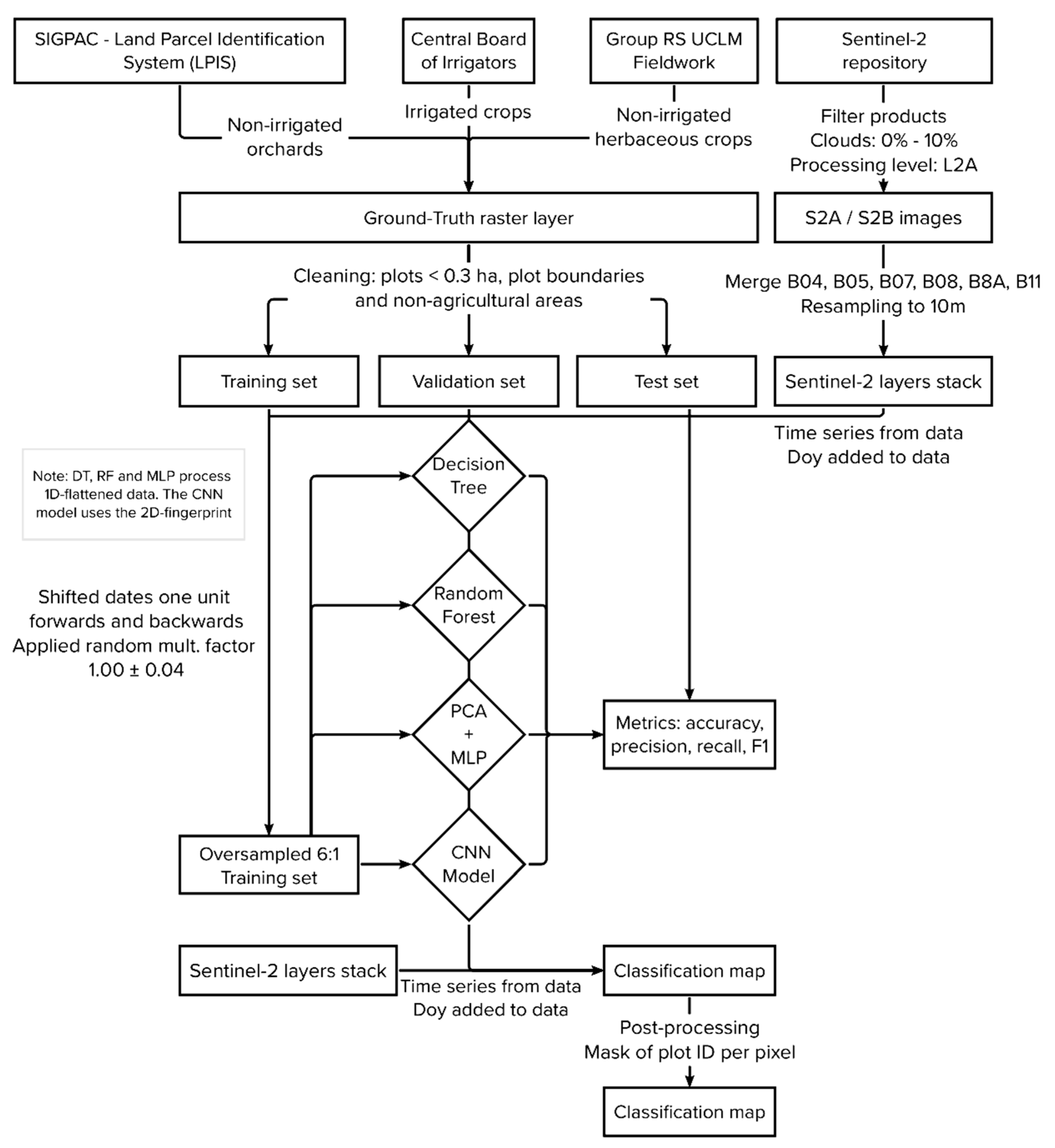
In this article, we propose a model for land use classification that requires few images and offers good results in the area of our focus. While some previous models work at the image level, carrying out segmentation and requiring large datasets, we consider that: (i) a pixel can contain enough information to successfully perform classification; (ii) part of this information lies in multispectral temporal patterns; and (iii) although such patterns are not especially complex, existing works based on random forest might not capture them, whereas others models, such as LTSM, are unnecessarily complex and require larger sequences. Based on these assumptions, we propose an approach that arranges the information corresponding to a pixel as a 2D yearly fingerprint and uses a convolution-based model (CNN) for the prediction. This approach can render multispectral temporal patterns more explicit and improve the classification. In fact, the state-of-the-art algorithms for time series classification are based on convolutions [35,36]. We also added a problem-specific process of oversampling, trying to deal with variations in phenology. We used this approach to perform (i) the classification of the main crop classes, focusing on herbaceous and woody crops, and (ii) discrimination between irrigated and non-irrigated areas.

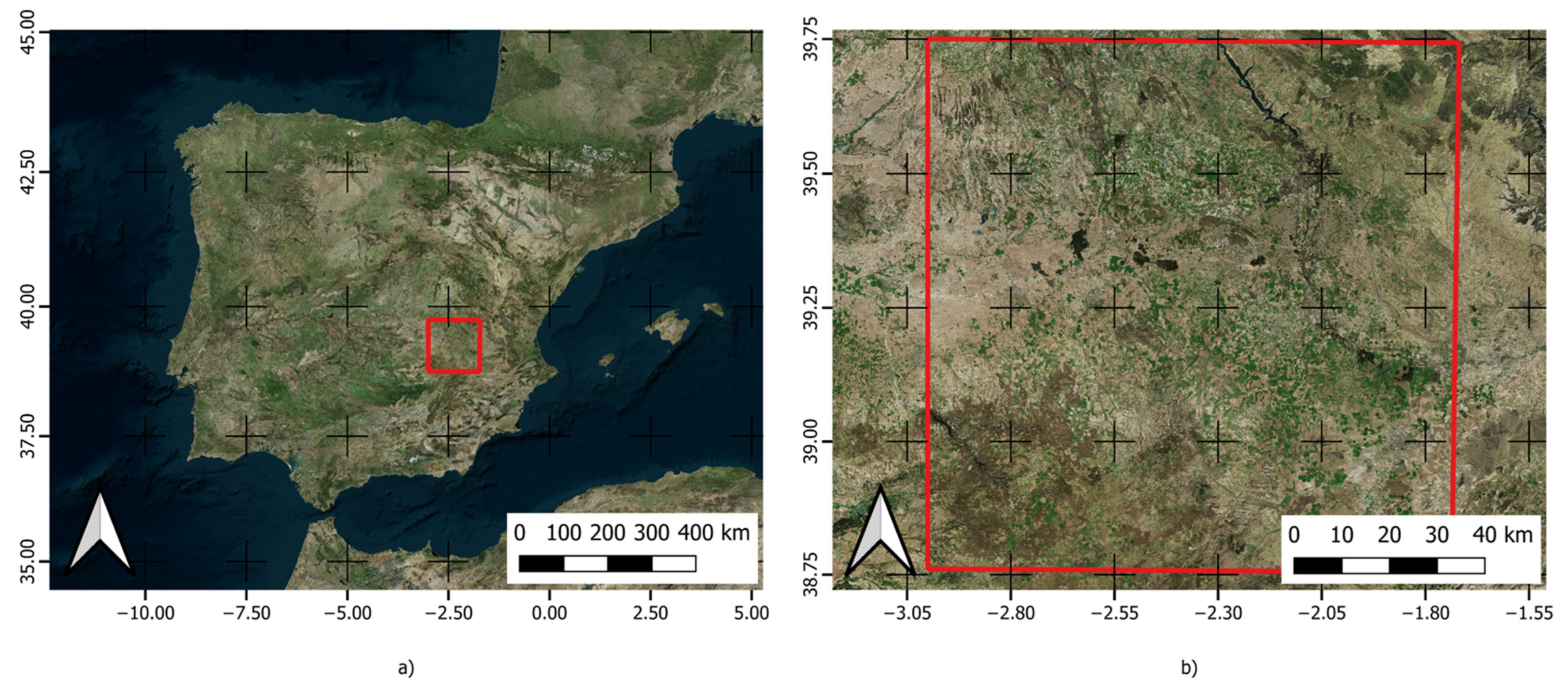
Therefore, a relevant contribution of this work is the consequent improvement in pixel-based land use classification with a small number of images by representing data as a 2D fingerprint and using a CNN model. We tested our proposal in a well-known agricultural area in the Mancha Oriental aquifer in Spain. Improvement regarding these issues is of great interest, as land use information is a basic input for water accounting [37], water footprint estimations for environmental management [38], and yield prediction modelling [39].

2. Materials and Methods

Figure 1 summarizes, in a workflow, the content of this section, showing how the satellite and labeled data are selected, gathered, and later processed to build, assess, and employ the model.

2.1. Input Data

Our study takes as its basis a set of 24 images from the year 2018, corresponding to different dates from March to October, as shown in

Table 1. Dates of the T30SWJ granule set of 24 Sentinel 2 images at level L2A, selected with a maximum of 10% cloud coverage in the study area.

2018
March	April	May	June	July	August	September	October
27	14, 26	4, 16	13, 18, 23	3, 8, 13, 18, 23, 28	2, 12, 17, 22, 27	1, 13, 21	3, 6

. The images were downloaded from the Copernicus Open Access Hub server, and we considered only those in which the percentage of clouds was below 10%, setting a processing level of L2A. This criterion reduces the noise introduced by the presence of clouds and shade on the surface. This set of images was used to generate spectral-temporal signatures.

Sentinel 2 data requires pre-processing, insofar as the information on the bands is stored in different files that have different resolutions. Thus, bands with the lowest resolution, which can range between 20 and 60 m, need to be resampled to obtain a resolution of 10 m so that they can all be merged into a single tiff file for each date (

Table 2. Pre-processed resampled tiff image correspondence with Sentinel-2 bands.

#	Sentinel-2 Band	Original Res.	Target Res.	Wavelength (µm)
1	B02	10 m	10 m	0.490
2	B03	10 m	10 m	0.560
3	B04	10 m	10 m	0.665
4	B08	10 m	10 m	0.842
5	B05	20 m	10 m	0.705
6	B06	20 m	10 m	0.740
7	B07	20 m	10 m	0.783
8	B8A	20 m	10 m	0.865
9	B11	20 m	10 m	1.610
10	B12	20 m	10 m	2.190
11	B01	60 m	10 m	0.443
12	B09	60 m	10 m	0.945

). In addition, those pixels belonging to plots with areas under 0.3 ha were excluded from the study because of the limitation of the resolution of the satellite.

As deep learning enables the identification of more patterns from the raw features of the input data, the experts’ need for the introduction of new features built using original data with their knowledge, such as NDVI, is not particularly relevant, although it may lead to an improvement in some cases. As a matter of fact, this characteristic results in a clear advantage when compared to traditional methods [40]. In this proposal, the information is managed at the pixel level, so that each one of them is treated as a single and independent entity that is formed by the bands of information for the 24 selected dates. Moreover, considering previous works that stated the importance of spectral information [41], the number of bands used in this practical case was reduced from 12 bands to 6 bands, without any impact on the performance of the model, in order to optimize the computational resources in terms of the memory usage. The chosen bands, ordered by relevance, are B4, B8, B11, B8A, B7, and B5. Figure 2 shows both the NDVI sequence and the 2D fingerprint at a pixel level that corresponds to the land use of forage irrigated crops. The NDVI sequence is an index that can be interpreted by agronomic experts and allows them to build models according to their knowledge of the phenology of the crops, as the curve is correlated with the different growing stages [42,43], although the classification process using only NDVI does not consider all the available relevant information. In contrast, the representation of data at a pixel level as a 2D fingerprint carries the most important information, and it can be processed as an image by employing algorithms, such as CNNs, to efficiently find patterns and relationships between the bands and the different dates.

2.2. Area of Study

The area of study (Figure 3) is located in Albacete, Spain. For this area, the Sentinel-2 granule corresponds to T30SWJ. This location was selected due to the variety of land use, the availability of images with a low percentage of clouds, and the high expertise in land use classification regarding this area, with many national and international projects having been carried out in this test location and accurate field information being available from recent years [44,45].

The ground truth data are composed of information corresponding to the year 2018. They were provided by the following sources: (i) the Central Board of Irrigators, which contributed the irrigated plot data, obtained from fieldwork; (ii) the non-irrigated data provided by the Remote Sensing and GIS Group (Albacete, University of Castilla-La Mancha), based on their fieldwork; and (iii) SIGPAC, the national Land Parcel Identification System in Spain, which provided non-irrigated woody crop field information based on the farmers’ reports. SIGPAC information is reliable, since it corresponds to long-term crops that are intended to be cultivated over many years. In order to facilitate the assessments by scientists, agronomists and technicians in the area, according to the experience derived from previous classification projects focusing on agronomic and sustainable criteria and considering the aim to deal with water management, the categories shown in

Table 3. Land use classification categories.

#	Class	Hectares	%
1	Forage irrigated	4331	2.75
2	Spring irrigated	28,473	18.05
3	Spring irrigated Chinese garlic	6483	4.11
4	Spring irrigated purple garlic and horticulture	2852	1.81
5	Late spring irrigated	1842	1.17
6	Summer irrigated, low cover and horticulture	5572	3.53
7	Summer irrigated, high coverage	7160	4.54
8	Irrigated alfalfa	5365	3.40
9	Double crop	6904	4.38
10	Non-irrigated	7275	4.61
11	Bare soil	1098	0.70
13	Irrigated vineyard	9704	6.15
15	Non-irrigated vineyard	37,263	23.62
16	Irrigated olive trees	753	0.48
18	Non-irrigated olive trees	9266	5.87
19	Irrigated shell fruit trees	6368	4.04
21	Non-irrigated shell fruit trees	14,915	9.45
22	Irrigated fruit trees	175	0.11
24	Non-irrigated fruit trees	1972	1.25
	Total	157,771

were selected, distinguishing between irrigated and non-irrigated crops.

2.3. Selected Models: Decision Tree, Random Forest, Multilayer Perceptron, and Neural Networks

Some existing works carry out LUC by means of a set of rules built and tuned by experts [18]. These can be represented as a decision tree. Therefore, the first method selected to test the proposed classification scheme was the automatic learning of decision trees, where nodes represent conditions for the variables and leaves correspond to classes. These models are popular because of their low learning complexity, being carried out with a greedy algorithm, and because they essentially perform a selection of relevant features, discarding the rest [46].

Depending on the problem, decision trees can under- or overfit the training data. In general, ensemble models are frequently used in machine learning because they can deal with both problems at the same time. One of the most popular ensembles is the random forest, which combines bagging and randomly built decision trees [47].

Neural networks (NN) are models inspired by the structure of biological neural networks. An artificial neuron is a simple processing unit characterized by a set of weights. It receives a finite set of values—i.e., as many as there are weights—as the input, creates a weighted linear combination of them, and applies an activation function to the resulting value to generate an output. In their most basic form, neural networks (NN) are composed of several layers of artificial neurons arranged as an input layer, an output layer, and several hidden layers. Each neuron in the input layer processes the input data, producing an output value. Then, for all the remaining neurons, the input values correspond to the outputs produced in the previous layer. Lastly, the values generated by the neuron of the output layer are predefined labels that correspond to the labels or target variable. This is called forward propagation. Activation functions, such as sigmoid or hyperbolic tangent, together with the use of hidden layers, allow neural networks to represent complex, non-linear decision functions [48]. Multilayer perceptrons (MLPs) are the most basic type of fully connected feedforward neural network [49]. In this work, MLPs were first tested on their own but did not obtain acceptable results. Finally, the performance of this model was remarkably improved by applying principal component analysis (PCA) [50]. This method captures linear dependences among the input features and projects data onto a set of components, retaining most of its variance while reducing dimensionality and noise, which, in this case, can be produced by the presence of clouds [51].

The last developed model is based on the use of CNNs to extract the temporal-multispectral patterns from time series. As stated, the data were prepared as 2D images which contain temporal and multispectral data on each of their axes. Therefore, this enables the application of two-dimensional CNNs, allowing them to identify those patterns in a 2D array. This model (Figure 4) is composed of six initial Conv2D layers, which receive input data, with dimensions 24 dates × 7 bands, and reduce the number of parameters for the next layers. Usually, pooling layers are used after each convolution to reduce the spatial dimension of the feature maps, which was not considered in this concrete case so as to preserve the information. Convolutions of 1 × 7, 3 × 3, and 1 × 5 are considered in this model; thus, it can identify the changes over time for each band and the relationships between them. Finally, the flattened output of the Conv2D layers is used as an input for the final four dense hidden layers, in which L2 regularization is also applied to avoid the overfitting of the data.

For this work, we used the machine learning methods implemented in Scikit-Learn. This is a state-of-the-art machine learning method, used in python, as it provides many tools for tasks such as the use of models for classification, regression, clustering, dimensionality reduction, etc. [52]. We also used TensorFlow to implement the convolutional neural networks. Its particular purpose is focused on deep neural networks, and it provides tools and options that can be used to configure and build deep learning models [53].

2.4. Data Preparation: Hold-Out, Oversampling, and Post-Processing

The whole dataset is composed of sequential data corresponding to the evolution of the spectrum of each pixel over a year. We used a hold-out procedure [54], dividing the data into one subset for the model training; another, the validation set, for the model tunning; and the last, the test set, for the model evaluation.

Table 4. Dataset divided for land use classification.

Crop and Irrigation Soil Classification
	Pixels	%
Training set	119,364	1.00
Validation set	834,753	6.97
Test set	11,030,736	92.03

shows the sizes of the resulting sets. Although larger training datasets help us to both detect more complex patterns and prevent overfitting, learning curves do not show improvement if the proportion of data used for training is increased above 1% of the data. On the other hand, test sets are usually smaller than training sets because of the lack of data. However, this leads to estimations affected by randomness and noise. In this scenario, models can be evaluated with the whole set of (remaining) pixels. This renders the estimation of the performance indicators far more robust.

We also improved the training with synthetic data. For the purpose of capturing the variations in the phenology over different years due to environmental and management conditions, we also propose a methodology based on oversampling, generating new instances by assigning the readings corresponding to pixels of the previous or later capture date. In addition to this, the data were replicated and multiplied by a random factor of 1.00 ± 0.04 to introduce an acceptable range of variation, which can represent the scenarios at different times or locations. Moreover, when the data are loaded, the day of the year is normalized using the sine function, so that it has a temporal reference, with values between zero and one. Thus, the first and last days of the year have similar values near zero.

Additionally, since our focus was on pixel-based classification, a procedure was proposed to integrate it into a plot level. This post-processing step consisted of overlaying the plot vector layer with the raster image of the classification, assigning the majority class to the pixels corresponding to each plot. The procedure consisted of checking every plot. When the majority class among the classified pixels for that plot is over 40%, it proceeds to verify the rest of the classes of the classified pixels. In a case where the previous condition holds, and the pixel representation of a minority class is under 25%, those underrepresented pixels, which are considered to be misclassified, change their classification value to the majority class of the pixels in that plot.

2.5. Evaluation

The classes are unbalanced in the dataset, as can be observed from the areas and the percentages in Table 3. This dataset was treated by selecting a minimum number of instances of each class for the training set and considering the weights of each class so as to adjust their importance during the training. In this way, the models do not overfit the most representative classes, and their ability to predict the classes in which there are fewer samples is improved [55].

In order to assess the results, the following metrics were applied to the validation and test sets [56,57]: (i) accuracy, which shows the rate of correct predictions (CP) made by the model and is the ratio between the number of CP divided by the number of total cases (TC); (ii) recall, which is the number of total correctly predicted positive results (TP) divided by the total number of cases which should be detected as positive (sum of the false negatives, FN and TP); (iii) precision, which expresses the rate between the TP and the sum of the TP and false negatives (FN); and the (iv) F1-score, which is the harmonic mean between the precision and recall, with values within the range of [0, 1]. The recall, precision, and F1-Score are defined for the binary classification and are calculated for each class, considering the class in question as positive and the rest as negative. The summary results reported for each model correspond to the weighted average of the metrics, whose weights correspond to the number of pixels of each class.

$$Accuracy=\frac{CP}{TC},$$

(1)

$$Recall=\frac{TP}{\left(FN+TP\right)},$$

(2)

$$Precision=\frac{TP}{\left(FP+TP\right)},$$

(3)

$$F_{1}Score=2·\frac{Precision·Recall}{Precision+Recall}.$$

(4)

3. Results

The selected models were applied to the test set to assess them and validate their performance according to the statistics proposed. Thus far, this section has shown how traditional machine and deep learning models perform in these tasks.

3.1. Decision Tree

The report in

Table 5. Land use classification: decision tree.

Class	Precision	Recall	F1	Support
Forage irrigated	0.61	0.68	0.64	343,643
Spring irrigated	0.91	0.90	0.91	2,373,450
Spring irrigated Chinese garlic	0.82	0.83	0.82	546,212
Spring irrigated purple garlic and horticulture	0.88	0.90	0.89	235,297
Late spring irrigated	0.64	0.73	0.68	141,147
Summer irrigated, low cover and horticulture	0.84	0.82	0.83	455,175
Summer irrigated, high coverage	0.89	0.87	0.88	585,448
Irrigated alfalfa	0.94	0.91	0.93	445,925
Double crop	0.87	0.80	0.83	572,968
Herbaceous non-irrigated	0.62	0.58	0.60	569,945
Bare soil	0.49	0.71	0.58	77,114
Irrigated vineyard	0.54	0.51	0.53	734,295
Non-irrigated vineyard	0.74	0.72	0.73	2,111,911
Irrigated olive trees	0.41	0.57	0.48	43,715
Non-irrigated olive trees	0.38	0.34	0.36	321,381
Irrigated shell fruit trees	0.51	0.51	0.51	514,900
Non-irrigated shell fruit trees	0.50	0.58	0.54	888,792
Irrigated fruit trees	0.20	0.78	0.32	6974
Non-irrigated fruit trees	0.14	0.11	0.12	62,444
Accuracy			0.73	11,030,736
Weighted avg.	0.74	0.73	0.74

shows the expected behavior regarding the low complexity of this algorithm, which is not capable of training a robust model. Considering each class, the F1 is slightly higher in the herbaceous irrigated crops than in the herbaceous non-irrigated crops, bare soil, and orchards. There are specific classes, such as bare soil or irrigated fruit trees, that are correctly detected, as the recall shows a higher value. However, they are not well classified, as there is confusion with regard to the other classes, as the precision is low. This results in a low F1 because those previous metrics are not balanced. According to these metrics and the achieved 73% overall accuracy, this model lacks robustness.

3.2. Random Forest

Random forest has a great modelling power but, at the same time, it maintains a low variance and does not usually produce overfitting. The report in

Table 6. Land use classification: random forest.

Class	Precision	Recall	F1	Support
Forage irrigated	0.90	0.80	0.85	343,643
Spring irrigated	0.95	0.95	0.95	2,373,450
Spring irrigated Chinese garlic	0.89	0.95	0.92	546,212
Spring irrigated purple garlic and horticulture	0.97	0.96	0.97	235,297
Late spring irrigated	0.97	0.80	0.87	141,147
Summer irrigated, low cover and horticulture	0.91	0.93	0.92	455,175
Summer irrigated, high coverage	0.97	0.93	0.95	585,448
Irrigated alfalfa	0.97	0.97	0.97	445,925
Double crop	0.96	0.91	0.93	572,968
Herbaceous non-irrigated	0.79	0.74	0.76	569,945
Bare soil	0.86	0.79	0.82	77,114
Irrigated vineyard	0.75	0.52	0.61	734,295
Non-irrigated vineyard	0.74	0.87	0.80	2,111,911
Irrigated olive trees	0.87	0.64	0.74	43,715
Non-irrigated olive trees	0.63	0.34	0.44	321,381
Irrigated shell fruit trees	0.78	0.64	0.70	514,900
Non-irrigated shell fruit trees	0.57	0.73	0.64	888,792
Irrigated fruit trees	0.68	0.89	0.77	6974
Non-irrigated fruit trees	0.35	0.14	0.20	62,444
Accuracy			0.83	11,030,736
Weighted avg.	0.83	0.83	0.83

shows the expected improvement compared to the decision tree. Thus, the overall accuracy reaches 83%, and the average F1 also reaches 83%. However, the assessment needs to be performed considering each class. The F1 is above 85% in the herbaceous irrigated crops, whereas the model is not as accurate in distinguishing the bare soil or herbaceous non-irrigated crops. Even so, it reaches an 80% F1 for those two classes. Regarding the orchards, these results are one step ahead of the previous ones, despite the fact that there is still room for refinement. The F1 of the irrigated herbaceous crops is over 90%, high enough to be used to identify those classes with acceptable confidence in an application scenario.

3.3. Multilayer Perceptron with PCA

The multilayer perceptron (MLP) algorithm was applied on its own, without preprocessing or cleaning the data, and we found that the model performed poorly. The application of PCA to the spectro-temporal sequences resulted in a notable gain in the performance of the MLP in the training process, with the advantage of its ability to reduce the number of features per sample and the noise of the dataset. As shown in

Table 7. Land use classification: MLP + PCA.

Class	Precision	Recall	F1	Support
Forage irrigated	0.86	0.85	0.86	343,643
Spring irrigated	0.96	0.94	0.95	2,373,450
Spring irrigated Chinese garlic	0.95	0.95	0.95	546,212
Spring irrigated purple garlic and horticulture	0.97	0.98	0.97	235,297
Late spring irrigated	0.88	0.92	0.90	141,147
Summer irrigated, low cover and horticulture	0.93	0.93	0.93	455,175
Summer irrigated, high coverage	0.96	0.94	0.95	585,448
Irrigated alfalfa	0.97	0.97	0.97	445,925
Double crop	0.93	0.94	0.94	572,968
Herbaceous non-irrigated	0.81	0.80	0.81	569,945
Bare soil	0.86	0.95	0.90	77,114
Irrigated vineyard	0.72	0.70	0.71	734,295
Non-irrigated vineyard	0.86	0.85	0.85	2,111,911
Irrigated olive trees	0.70	0.83	0.76	43,715
Non-irrigated olive trees	0.70	0.55	0.62	321,381
Irrigated shell fruit trees	0.78	0.80	0.79	514,900
Non-irrigated shell fruit trees	0.72	0.79	0.76	888,792
Irrigated fruit trees	0.39	0.96	0.56	6974
Non-irrigated fruit trees	0.22	0.33	0.26	62,444
Accuracy			0.87	11,030,736
Weighted avg.	0.87	0.87	0.87

, the most basic neural network outperforms the results from the decision tree and random forest, with an 87% weighted F1. Observing the F1 in each class, it can be inferred that both the precision and the recall are balanced, with promising results in the case of herbaceous irrigated crops.

3.4. Convolutional Neural Network

The report on the crop classification (

Table 8. Land use classification CNN. Pixel-based.

Class	Precision	Recall	F1	Support
Forage irrigated	0.93	0.93	0.93	343,643
Spring irrigated	0.97	0.97	0.97	2,373,450
Spring irrigated Chinese garlic	0.97	0.96	0.97	546,212
Spring irrigated purple garlic and horticulture	0.98	0.98	0.98	235,297
Late spring irrigated	0.95	0.96	0.95	141,147
Summer irrigated, low cover and horticulture	0.96	0.95	0.96	455,175
Summer irrigated, high coverage	0.97	0.96	0.97	585,448
Irrigated alfalfa	0.98	0.98	0.98	445,925
Double crop	0.96	0.96	0.96	572,968
Herbaceous non-irrigated	0.89	0.89	0.89	569,945
Bare soil	0.89	0.98	0.93	77,114
Irrigated vineyard	0.82	0.79	0.80	734,295
Non-irrigated vineyard	0.89	0.89	0.89	2,111,911
Irrigated olive trees	0.73	0.91	0.81	43,715
Non-irrigated olive trees	0.66	0.64	0.65	321,381
Irrigated shell fruit trees	0.87	0.87	0.87	514,900
Non-irrigated shell fruit trees	0.82	0.82	0.82	888,792
Irrigated fruit trees	0.52	0.97	0.67	6974
Non-irrigated fruit trees	0.31	0.41	0.36	62,444
Accuracy			0.91	11,030,736
Weighted avg.	0.91	0.91	0.91

) with the use of deep learning shows a substantial improvement compared to the previous results. In this case, the CNNs behaved as expected by recognizing temporal patterns in the time series of the reflectance bands, represented as a 2D array. In other words, the temporal fingerprint per pixel is treated as an image. This raises the overall accuracy to 91%, performing better than the other models. The highest performance is obtained in irrigated herbaceous crops, with the F1 scores ranging from 93% to 98%. As for the non-irrigated herbaceous crops and bare soil, the F1 is around 90%, significantly higher than the rest of the presented models. Regarding orchards, it shows the best performance in the detection of vineyard and shell fruit trees, with an F1 between 80% and 89%. In the case of olive trees, the detection is better, with an F1 of 81% if irrigation is present and 65% if not. The F1 drops dramatically in the classes of fruit trees, not surpassing 67%. This is due to the lower number of pixels of these classes in the dataset. This issue will be explained further in the discussion. A sample of the classification is included in Figure 5. Figure 6 shows the results of the classification in this area compared to the available ground truth data.

Considering the lower F1 in the categories corresponding to orchards, it is worth verifying this in the confusion matrix (Figure 7). As can be observed in detail, those cases of misclassification mainly refer to crops of the same two major aggregated categories, herbaceous crops and orchards, with no mismatch between them. Moreover, it is also relevant that irrigated crops tend to be misclassified, with other irrigated crops and non-irrigated crops repeating this same pattern. Therefore, we considered using the same architecture to build a model with the sole purpose of identifying irrigated soil as an aggregated category.

3.5. Identification of Irrigated Crops

As can be observed, the performance of the model based on CNNs in detecting irrigated crops separately seems to be high. The original categories were grouped into three classes, irrigated, non-irrigated, and bare ground, to build and train another model with the same architecture. The results (

Table 9. Classification of irrigated, non-irrigated, and bare ground. Pixel-based.

Class	Precision	Recall	F1	Support
Irrigated	0.97	0.96	0.96	6,999,149
Non-irrigated	0.93	0.95	0.94	3,954,473
Bare ground	0.92	0.98	0.95	77,114
Accuracy			0.95	11,030,736
Weighted avg.	0.95	0.95	0.95

) for the identification of the irrigated soil are outstanding, since the most relevant class is the one corresponding to irrigated crops, and 96% of pixels are detected, as the recall shows. At the same time, the model prediction is right 97% of the time, when it classifies a pixel as irrigated. A sample of the classification is included in Figure 8. Both the overall accuracy and the average F1-score are 0.95.

3.6. Analysis at the Plot Level

Since the results of the deep neural network with the use of convolutional layers offer the best statistics among all the tested models, the previously exposed post-processing algorithm was applied to the classification generated using the CNN, thereby integrating the pixel-based classification into a plot level. This resulted in a slight overall improvement (

Table 10. Land use classification CNN. Post-processing.

Class	Precision	Recall	F1	Support
Forage irrigated	0.91	0.90	0.91	343,643
Spring irrigated	0.94	0.97	0.95	2,373,450
Spring irrigated Chinese garlic	0.96	0.93	0.95	546,212
Spring irrigated purple garlic and horticulture	0.96	0.95	0.96	235,297
Late spring irrigated	0.93	0.84	0.88	141,147
Summer irrigated, low cover and horticulture	0.94	0.91	0.93	455,175
Summer irrigated, high coverage	0.97	0.93	0.95	585,448
Irrigated alfalfa	0.96	0.97	0.96	445,925
Double crop	0.92	0.94	0.93	572,968
Herbaceous non-irrigated	0.93	0.93	0.93	569,945
Bare soil	0.94	1.00	0.97	77,114
Irrigated vineyard	0.88	0.84	0.86	734,295
Non-irrigated vineyard	0.89	0.93	0.91	2,111,911
Irrigated olive trees	0.84	0.94	0.89	43,715
Non-irrigated olive trees	0.76	0.64	0.69	321,381
Irrigated shell fruit trees	0.92	0.93	0.92	514,900
Non-irrigated shell fruit trees	0.87	0.86	0.87	888,792
Irrigated fruit trees	0.72	0.99	0.83	6974
Non-irrigated fruit trees	0.45	0.43	0.44	62,444
Accuracy			0.92	11,030,736
Weighted avg.	0.91	0.92	0.91

), which is mainly noticeable for the orchards, with a higher F1-score, whereas it is slightly lower in the case of the herbaceous irrigated crops. A sample of the classification is included in Figure 9.

After applying post-processing, in the case of the classification of irrigated crops, the results were slightly improved compared to those obtained using the base algorithm, as shown in

Table 11. Classification of irrigated, non-irrigated, and bare ground. Post-processing.

Class	Precision	Recall	F1	Support
Irrigated	0.98	0.97	0.98	6,999,149
Non-irrigated	0.95	0.96	0.96	3,954,473
Bare ground	0.96	1.00	0.98	77,114
Accuracy			0.97	11,030,736
Weighted avg.	0.97	0.97	0.97

.

The recall shows a 97% accuracy in detecting the irrigated pixels, whereas 98% of the pixels classified within the irrigated category actually correspond to that class. A sample of the classification is included in Figure 10.

4. Discussion

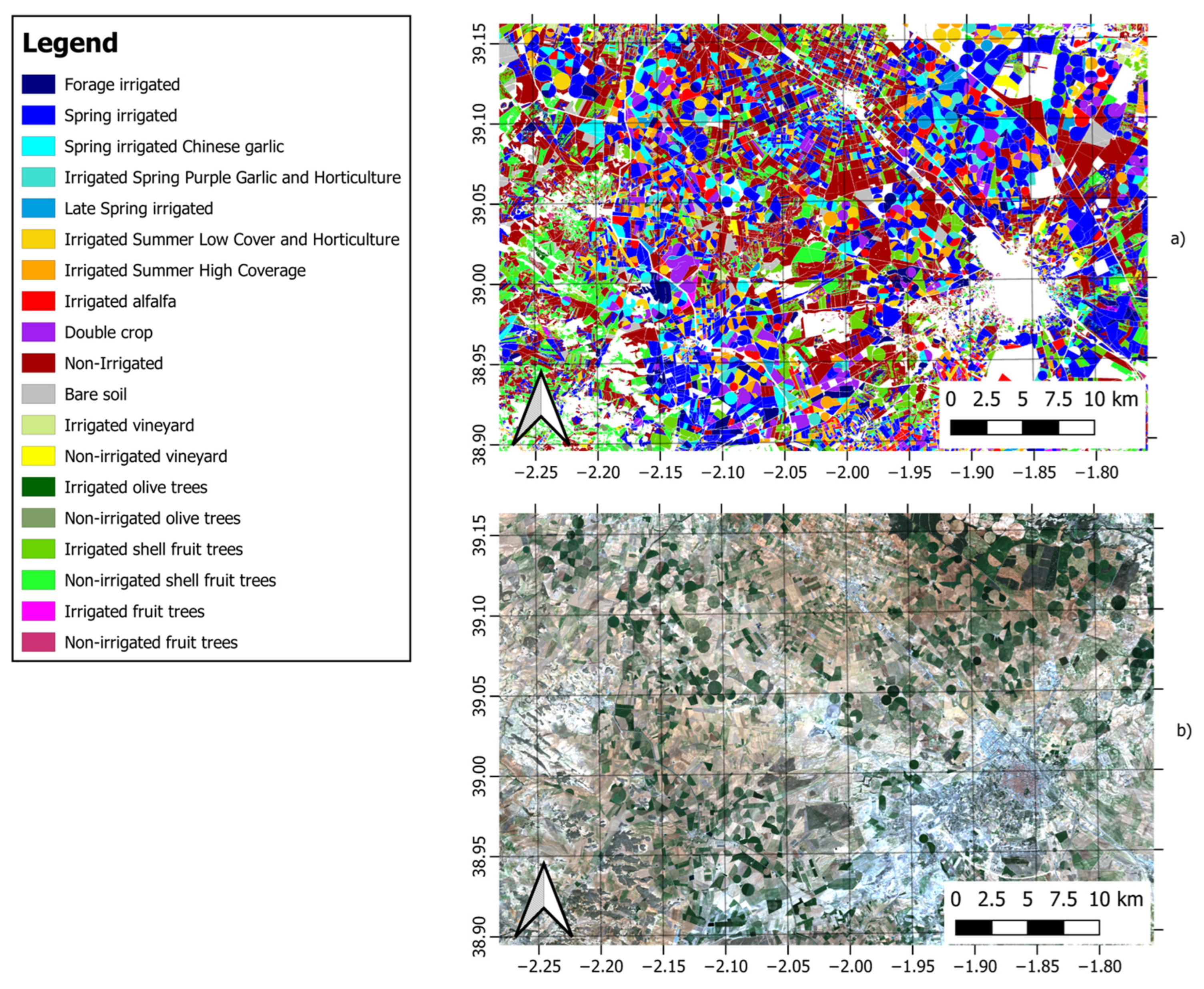
The core information for the crop classification comes from the Sentinel 2A and 2B constellations of the Copernicus program, which, nowadays, provide a high temporal and spatial resolution. A total of 24 images gathered on different dates from March to October were used. Despite observing a considerable time gap between May and June in this application, such a situation did not affect the performance of the model, as shown by the results. Additional data from different sources could be added, such as Landsat or national orthophotography program images and local sensors, so as to provide biophysical variables. For operational purposes, according to the computational resources, and to ensure the future scalability to other areas, Sentinel-2 sensors provide enough information for a successful classification for the purpose of pursuing an automatic process.

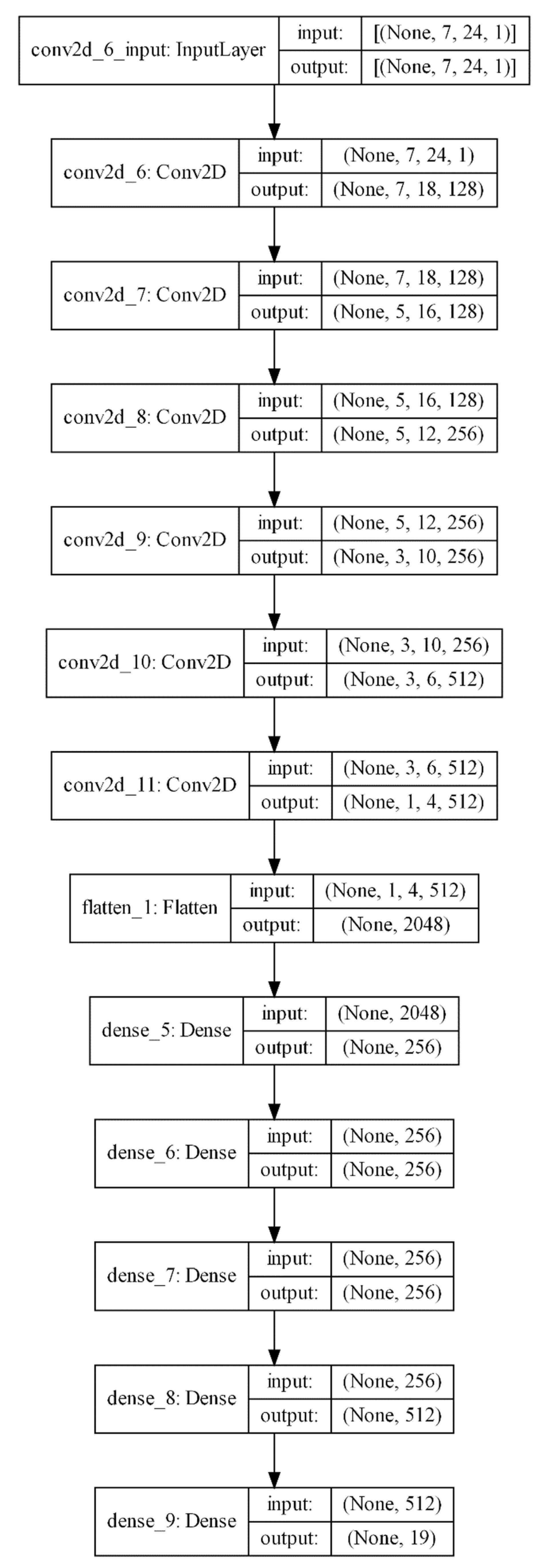
Our main objective was to represent the sequential data as a 2D spectro-temporal fingerprint of each pixel, which is particularly interesting with respect to its processing with machine learning. Therefore, it was tested using several algorithms, including CNNs, reducing the number of parameters for the fully connected layers and thus obtaining an enhancement of the speed and a reduction in the complexity of the model used to train and evaluate the data. The process of classification, designed to generate a land use cover, considers only the multispectral and temporal dimensions of the information at the pixel level.

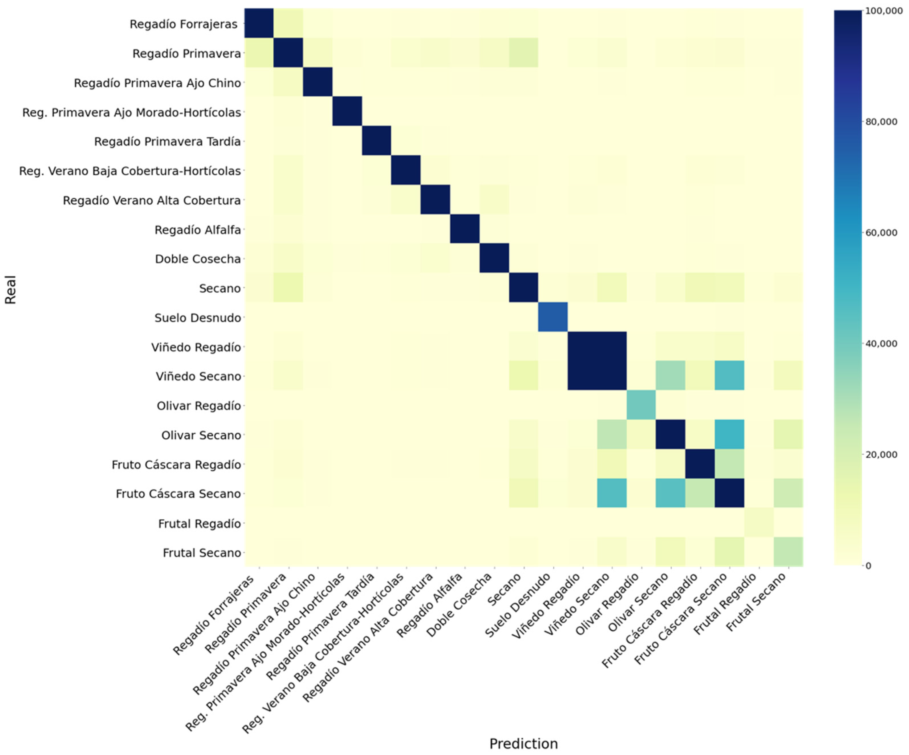
The convolutional neural network output was compared to those generated using other, simpler algorithms in global terms (

Table 12. Statistics for the comparison of the five selected models used to identify 19 classes.

Model	Metrics
	19 Classes Accuracy	19 Classes Weighted Avg. F1	Irrigation Detection Accuracy	Irrigation Detection Weighted Avg. F1	Fitting Time (s)	Prediction Time Per Million Samples (s)
Decision Tree	73%	74%			448	0.60
Random Forest	83%	83%			257	12.74
PCA + MLP	87%	87%			1505	11.69
CNN	91%	91%	95%	95%	11,576	13.76
CNN w/Postprocessing	92%	91%	97%	97%

) and compared by considering each separate class (

Table 13. Comparison of F1s for each model per class.

Class	F1
	DT	RF	PCA + MLP	CNN
Forage irrigated	0.64	0.85	0.86	0.93
Spring irrigated	0.91	0.95	0.95	0.97
Spring irrigated Chinese garlic	0.82	0.92	0.95	0.97
Spring irrigated purple garlic and horticulture	0.89	0.97	0.97	0.98
Late spring irrigated	0.68	0.87	0.90	0.95
Summer irrigated, low cover and horticulture	0.83	0.92	0.93	0.96
Summer irrigated, high coverage	0.88	0.95	0.95	0.97
Irrigated alfalfa	0.93	0.97	0.97	0.98
Double crop	0.83	0.93	0.94	0.96
Herbaceous non-irrigated	0.60	0.76	0.81	0.89
Bare soil	0.58	0.82	0.90	0.93
Irrigated vineyard	0.53	0.61	0.71	0.80
Non-irrigated vineyard	0.73	0.80	0.85	0.89
Irrigated olive trees	0.48	0.74	0.76	0.81
Non-irrigated olive trees	0.36	0.44	0.62	0.65
Irrigated shell fruit trees	0.51	0.70	0.79	0.87
Non-irrigated shell fruit trees	0.54	0.64	0.76	0.82
Irrigated fruit trees	0.32	0.77	0.56	0.67
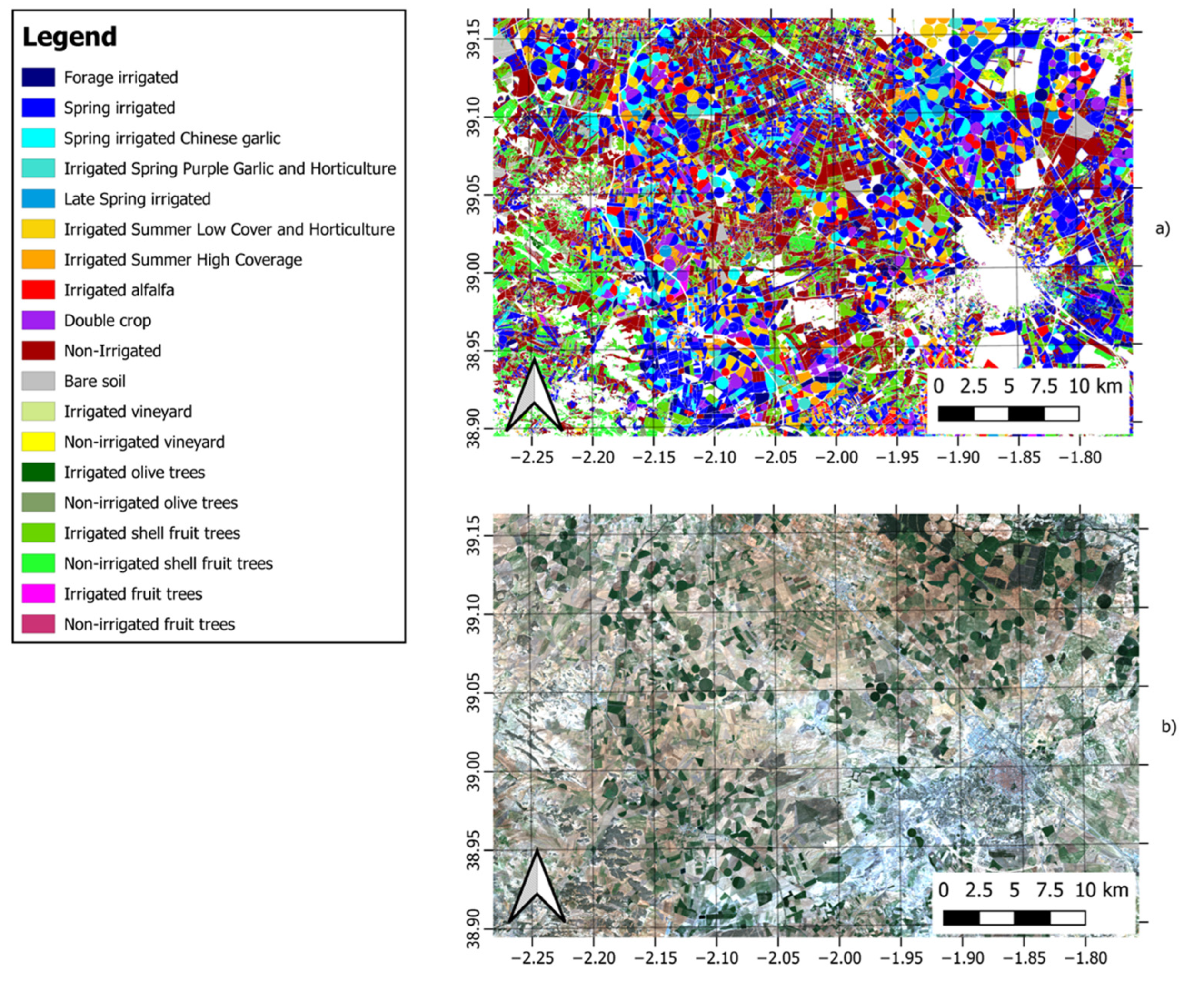
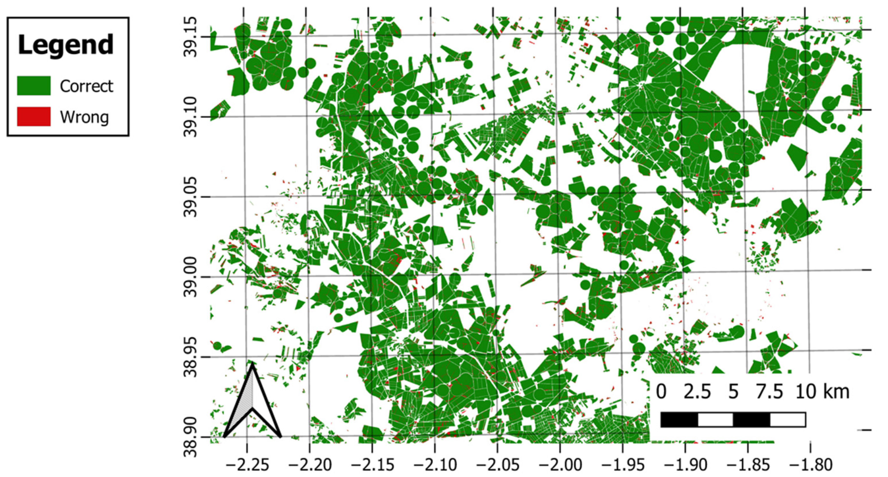
Non-irrigated fruit trees	0.12	0.20	0.26	0.36

). CNNs were proved to outperform any other model applied to the experimental data considered in this study with a similar prediction time. Since the training phase can only take place once the model has been updated, the improvement in global accuracy highly compensates for the training time, which is important for generating reliable land use classification maps. Both the overall accuracy and weighted average F1 are affected by all the results achieved for every class. In general, the performance of all the models considered is high. However, considering the resolution of the satellite images, we expected this to result in a slightly lower performance in the case of orchards. The mismatches between these classes correspond mainly to the same aggregated categories distinguishing between irrigated and non-irrigated crops. Considering the importance of identifying irrigated crops, a specific model for this purpose was considered, using the same architecture, to identify the irrigated land use, showing a 95% accuracy and a 95% F1, whereas it increased to 97% for both metrics when post-processing was applied.

According to the proposals shown in

Table 14. Previous proposals’ overall performance.

Proposal	RS	Features	Model	Accuracy	Classes
Ours	Sentinel-2	BOA ref.	Conv2D	91%	19
Portalés-Julià et al. [32]	Sentinel-2	Ref. and BSI	Bi-LSTM	98.2%	9
Campos-Taberner et al. [31]	Sentinel-2	Ref. and NDVI	Bi-LSTM	98.6%	16
Fan et al. [58]	Sentinel-2	BOA ref.	RF	96–98%	9
Zhong et al. [23]	Landsat	EVI	Conv1D	85.5%	14
Rußwurm and Körner [30]	Sentinel-2	TOA ref.	Bi-ConvLSTM	89.6%	17
Hao et al. [19]	MODIS	Phenological metrics	RF	89%	6
Foerster et al. [13]	Landsat	NDVI	DT	73%	11

, different types of models can be used in land use classification. These include traditional models based on decision trees and random forests, which constitute one of the most successful machine learning methods and deep learning models based on the use of recurrent neural networks, such as long short-term memory and convolutional neural networks.

Similar works applied to a set of images with pixel sizes larger than the plot showed a low accuracy of 50% in crop classification in some areas because of the presence of trees in the fields and the lack of resolution [9]. In light of this, the input information was filtered with a minimum threshold of 0.3 ha per plot, as explained in the methodology.

Hao et al. proposed a model which employs the phenological features obtained from a MODIS time series, whose resolution is lower than that of Landsat and Sentinel-2 images. They aimed to classify a reduced group of six classes, achieving an overall accuracy of 89% with a model based on random forest [19].

As Fan et al. demonstrated [58], the data volume of the Sentinel 2 images is large compared to the data provided by other satellites because of the medium-high resolution of the sensors. Therefore, we considered a similar solution, optimizing the volume of the training, while obtaining data to enable the model to learn without making the training set too large to be processed. Their model consists of a random forest that classifies the land use among nine classes. In this respect, it is necessary to point out that, when comparing algorithms, a smaller number of classes leads to simpler and more accurate models. In our proposal, we used CNNs inspired by Zhong et al.’s work [23], consisting of Conv1D layers that can be used to extract temporal patterns from an enhanced vegetation index (EVI) time series for 14 classes, whereas our model used Conv2D layers to extract temporal and multispectral patterns from the 2D fingerprint so as to classify 19 classes.

Rußwurm and Körner proposed a model whose input is derived from a Sentinel-2 top-of-atmosphere (TOA) time series and a maximum cloud level of 80%. They employed a Bi-ConvLSTM model, which obtained an 89.6% global accuracy in classifying 17 herbaceous crops, considering the spatial and temporal distribution [30]. In contrast, our proposal establishes a threshold of 10% for the presence of clouds in the image in order to consider it acceptable and employs a bottom-of-atmosphere (BOA) time series to perform the classification of both herbaceous crops and orchards, considering only the temporal distribution per pixel.

Campos-Taberner et al. presented a study which aimed to explain deep learning, in which they employed a bidirectional LSTM model [31]. Portalés-Julià et al. made improvements on their previous work, in which they continued using Bi-LSTM models [32], obtaining a 94.3% accuracy using random forests and an over 98% accuracy in their study area using Bi-LSTM networks. This may be the result of both the fact that the model did not discriminate irrigated areas and classified fewer classes. The use of LSTMs leads to higher computational costs in terms of time and resources compared to CNNs, which we used in our proposal with the aim of achieving an efficient model with a reduced number of parameters and a similar performance [36].

5. Conclusions

This work offered a comparison of different deep learning algorithms, which were used to identify 19 agricultural land use classes in the area of Albacete, Spain, a well-known testing area for the use of traditional decision tree algorithms. For this purpose, each pixel was characterized as a 2D fingerprint using a sequence of one-granule Sentinel 2 multispectral data over the year of 2018, developing traditional machine learning and deep neural networks models in order to classify the land use as herbaceous and orchards crops and consider whether they are irrigated or not. The best results were achieved by the deep neural networks containing two-dimensional convolutional layers (Conv2D), which outperformed the other accepted classifiers, such as random forests and multilayer perceptron, whose results were good in previous works. This model, based on CNNs, performs a pixel-based classification that analyzes the multispectral and temporal components, proving that it can obtain a high overall accuracy of 91%, regardless of the spatial distribution, by identifying multispectral-temporal patterns in the 2D pixel fingerprint. The accuracy of the model is higher in case of the herbaceous crops than the orchards, a which is even more notable if irrigation is applied. Additionally, the model we built to detect irrigated areas detects 97% of the irrigated areas with a 98% precision. Considering these achievements, a model based on two-dimensional convolutional layers shows promising results and potential to be applied to the area in question. This model is trained for a specific area; thus, the crops or the characteristics of other locations are not within its knowledge. For that purpose, additional possibilities for future work can be conceived in two different ways. The first option is to re-train the model with new samples from the other area, so that its weight changes to fit the new data. A second option is to take the layers of this model as a base in order to build a new one. These choices would allow for the application of transfer learning and take advantage of this previous work. This also implies an improvement, since experts in agronomy are currently performing heavy manual work in order to make classifications, which is a task that can take months to complete [18].

References

1. Dubois, O.; Faurès, J.; Felix, E.; Flammini, A.; Hoogeveen, J.; Pluschke, L.; Puri, M.; Ünver, O. The Water-Energy-Food Nexus. A New Approach in Support of Food Security and Sustainable Agriculture |Policy Support and Governance| Food and Agriculture Organization of the United Nations. Available online: https://www.fao.org/policy-support/tools-and-publications/resources-details/es/c/421718/ (accessed on 16 November 2021).
2. Deng, L.; Guo, S.; Yin, J.; Zeng, Y.; Chen, K. Multi-objective optimization of water resources allocation in Han River basin (China) integrating efficiency, equity and sustainability. Sci. Rep. 2022, 12, 798. [Google Scholar] [CrossRef] [PubMed]
3. Drakvik, E.; Kogevinas, M.; Bergman, Å.; Devouge, A.; Barouki, R.; on behalf of the HERA (Health and Environment Research Agenda) Consortium; Kogevinas, M.; Bergman, Å.; Drakvik, E. Priorities for research on environment, climate and health, a European perspective. Environ. Health 2022, 21, 37. [Google Scholar] [CrossRef] [PubMed]
4. Elliot, T.; Torres-Matallana, J.A.; Goldstein, B.; Babí Almenar, J.; Gómez-Baggethun, E.; Proença, V.; Rugani, B. An expanded framing of ecosystem services is needed for a sustainable urban future. Renew. Sustain. Energy Rev. 2022, 162, 112418. [Google Scholar] [CrossRef]
5. Matton, N.; Canto, G.S.; Waldner, F.; Valero, S.; Morin, D.; Inglada, J.; Arias, M.; Bontemps, S.; Koetz, B.; Defourny, P. An Automated Method for Annual Cropland Mapping along the Season for Various Globally-Distributed Agrosystems Using High Spatial and Temporal Resolution Time Series. Remote Sens. 2015, 7, 13208–13232. [Google Scholar] [CrossRef] [Green Version]
6. Gómez, C.; White, J.C.; Wulder, M.A. Optical remotely sensed time series data for land cover classification: A review. ISPRS J. Photogramm. Remote Sens. 2016, 116, 55–72. [Google Scholar] [CrossRef] [Green Version]
7. Leemhuis, C.; Thonfeld, F.; Näschen, K.; Steinbach, S.; Muro, J.; Strauch, A.; López, A.; Daconto, G.; Games, I.; Diekkrüger, B. Sustainability in the Food-Water-Ecosystem Nexus: The Role of Land Use and Land Cover Change for Water Resources and Ecosystems in the Kilombero Wetland, Tanzania. Sustainability 2017, 9, 1513. [Google Scholar] [CrossRef] [Green Version]
8. Sánchez, J.M.; Galve, J.M.; González-Piqueras, J.; López-Urrea, R.; Niclòs, R.; Calera, A. Downscaling MODIS land surface temperature to Sentinel-2 spatial resolution in the Barrax test site. SPIE 2019, 11174, 317–323. [Google Scholar]
9. Inglada, J.; Arias, M.; Tardy, B.; Hagolle, O.; Valero, S.; Morin, D.; Dedieu, G.; Sepulcre, G.; Bontemps, S.; Defourny, P.; et al. Assessment of an Operational System for Crop Type Map Production Using High Temporal and Spatial Resolution Satellite Optical Imagery. Remote Sens. 2015, 7, 12356–12379. [Google Scholar] [CrossRef] [Green Version]
10. Vuolo, F.; Neuwirth, M.; Immitzer, M.; Atzberger, C.; Ng, W.-T. How much does multi-temporal Sentinel-2 data improve crop type classification? Int. J. Appl. Earth Obs. Geoinf. 2018, 72, 122–130. [Google Scholar] [CrossRef]
11. Carrao, H.; Gonçalves, P.; Caetano, M. Contribution of multispectral and multitemporal information from MODIS images to land cover classification. Remote Sens. Environ. 2008, 112, 986–997. [Google Scholar] [CrossRef]
12. Friedl, M.A.; McIver, D.K.; Hodges, J.C.F.; Zhang, X.Y.; Muchoney, D.; Strahler, A.H.; Woodcock, C.E.; Gopal, S.; Schneider, A.; Cooper, A.; et al. Global land cover mapping from MODIS: Algorithms and early results. Remote Sens. Environ. 2002, 83, 287–302. [Google Scholar] [CrossRef]
13. Foerster, S.; Kaden, K.; Förster, M.; Itzerott, S. Crop type mapping using spectral-temporal profiles and phenological information. Comput. Electron. Agric. 2012, 89, 30–40. [Google Scholar] [CrossRef] [Green Version]
14. Revill, A.; Florence, A.; MacArthur, A.; Hoad, S.P.; Rees, R.M.; Williams, M. The Value of Sentinel-2 Spectral Bands for the Assessment of Winter Wheat Growth and Development. Remote Sens. 2019, 11, 2050. [Google Scholar] [CrossRef] [Green Version]
15. Huang, S.; Tang, L.; Hupy, J.P.; Wang, Y.; Shao, G. A commentary review on the use of normalized difference vegetation index (NDVI) in the era of popular remote sensing. J. For. Res. 2021, 32, 1–6. [Google Scholar] [CrossRef]
16. Silleos, N.; Misopolinos, N.; Perakis, K. Relationships between remote sensing spectral indices and crops discrimination. Geocarto Int. 1992, 7, 41–51. [Google Scholar] [CrossRef]
17. Gilabert, M.A.; González-Piqueras, J.; García-Haro, J. Acerca de los Indices de Vegetación. Rev. Teledetec. 1997, 8, 10. [Google Scholar]
18. Conrad, C.; Fritsch, S.; Zeidler, J.; Rücker, G.; Dech, S. Per-Field Irrigated Crop Classification in Arid Central Asia Using SPOT and ASTER Data. Remote Sens. 2010, 2, 1035–1056. [Google Scholar] [CrossRef] [Green Version]
19. Hao, P.; Zhan, Y.; Wang, L.; Niu, Z.; Shakir, M. Feature Selection of Time Series MODIS Data for Early Crop Classification Using Random Forest: A Case Study in Kansas, USA. Remote Sens. 2015, 7, 5347–5369. [Google Scholar] [CrossRef] [Green Version]
20. Immitzer, M.; Vuolo, F.; Atzberger, C. First experience with Sentinel-2 data for crop and tree species classifications in central Europe. Remote Sens. 2016, 8, 166. [Google Scholar] [CrossRef]
21. Hao, P.; Wang, L.; Niu, Z.; Aablikim, A.; Huang, N.; Xu, S.; Chen, F. The Potential of Time Series Merged from Landsat-5 TM and HJ-1 CCD for Crop Classification: A Case Study for Bole and Manas Counties in Xinjiang, China. Remote Sens. 2014, 6, 7610–7631. [Google Scholar] [CrossRef] [Green Version]
22. Zhou, F.; Aining, Z.; Townley-Smith, L. A data mining approach for evaluation of optimal time-series of MODIS data for land cover mapping at a regional level. ISPRS J. Photogramm. Remote Sens. 2013, 84, 114–129. [Google Scholar] [CrossRef]
23. Zhong, L.; Hu, L.; Zhou, H. Deep learning based multi-temporal crop classification. Remote Sens. Environ. 2019, 221, 430–443. [Google Scholar] [CrossRef]
24. Valueva, M.V.; Nagornov, N.N.; Lyakhov, P.A.; Valuev, G.V.; Chervyakov, N.I. Application of the residue number system to reduce hardware costs of the convolutional neural network implementation. Math. Comput. Simul. 2020, 177, 232–243. [Google Scholar] [CrossRef]
25. Li, X.; Wu, X. Constructing Long Short-Term Memory based Deep Recurrent Neural Networks for Large Vocabulary Speech Recognition. arXiv 2015, arXiv:Computer Science/1410.4281. [Google Scholar] [CrossRef]
26. Lyu, H.; Lu, H.; Mou, L. Learning a Transferable Change Rule from a Recurrent Neural Network for Land Cover Change Detection. Remote Sens. 2016, 8, 506. [Google Scholar] [CrossRef] [Green Version]
27. Mou, L.; Bruzzone, L.; Zhu, X.X. Learning Spectral-Spatial-Temporal Features via a Recurrent Convolutional Neural Network for Change Detection in Multispectral Imagery. IEEE Trans. Geosci. Remote Sens. 2019, 57, 924–935. [Google Scholar] [CrossRef] [Green Version]
28. Krizhevsky, A.; Sutskever, I.; Hinton, G.E. ImageNet classification with deep convolutional neural networks. Commun. ACM 2012, 2, 1097–1105. [Google Scholar] [CrossRef] [Green Version]
29. Rußwurm, M.; Korner, M. Temporal Vegetation Modelling Using Long Short-Term Memory Networks for Crop Identification from Medium-Resolution Multi-spectral Satellite Images. In Proceedings of the 2017 IEEE Conference on Computer Vision and Pattern Recognition Workshops (CVPRW), Honolulu, HI, USA, 21 July 2017; pp. 1496–1504. [Google Scholar]
30. Rußwurm, M.; Körner, M. Multi-Temporal Land Cover Classification with Sequential Recurrent Encoders. ISPRS Int. J. Geo Inf. 2018, 7, 129. [Google Scholar] [CrossRef] [Green Version]
31. Campos-Taberner, M.; García-Haro, F.J.; Martínez, B.; Gilabert, M.A. Deep learning for agricultural land use classification from Sentinel-2. Rev. Teledetec. 2020, 56, 35–48. [Google Scholar] [CrossRef]
32. Portalés-Julià, E.; Campos-Taberner, M.; García-Haro, F.J.; Gilabert, M.A. Assessing the sentinel-2 capabilities to identify abandoned crops using deep learning. Agronomy 2021, 11, 654. [Google Scholar] [CrossRef]
33. Ruiz, L.A.; Almonacid-Caballer, J.; Crespo-Peremarch, P.; Recio, J.A.; Pardo-Pascual, J.E.; Sánchez-García, E. Automated classification of crop types and condition in a mediterranean area using a fine-tuned convolutional neural network. Int. Soc. Photogramm. Remote Sens. 2020, 43, 1061–1068. [Google Scholar] [CrossRef]
34. Amani, M.; Kakooei, M.; Moghimi, A.; Ghorbanian, A.; Ranjgar, B.; Mahdavi, S.; Davidson, A.; Fisette, T.; Rollin, P.; Brisco, B.; et al. Application of Google Earth Engine Cloud Computing Platform, Sentinel Imagery, and Neural Networks for Crop Mapping in Canada. Remote Sens. 2020, 12, 3561. [Google Scholar] [CrossRef]
35. Dempster, A.; Petitjean, F.; Webb, G.I. ROCKET: Exceptionally fast and accurate time series classification using random convolutional kernels. Data Min. Knowl. Discov. 2019, 34, 1454–1495. [Google Scholar] [CrossRef]
36. Weytjens, H.; De Weerdt, J. Process Outcome Prediction: CNN vs. LSTM (with Attention). Int. Conf. Bus. Process Manag. 2020, 397, 321–333. [Google Scholar] [CrossRef]
37. Murmu, S.; Biswas, S. Application of Fuzzy Logic and Neural Network in Crop Classification: A Review. Aquat. Procedia 2015, 4, 1203–1210. [Google Scholar] [CrossRef]
38. Garrido-Rubio, J.; González-Piqueras, J.; Campos, I.; Osann, A.; González-Gómez, L.; Calera, A. Remote sensing–based soil water balance for irrigation water accounting at plot and water user association management scale. Agric. Water Manag. 2020, 238, 106236. [Google Scholar] [CrossRef]
39. Campos, I.; González-Gómez, L.; Villodre, J.; González-Piqueras, J.; Suyker, A.E.; Calera, A. Remote sensing-based crop biomass with water or light-driven crop growth models in wheat commercial fields. Field Crops Res. 2018, 216, 175–188. [Google Scholar] [CrossRef]
40. Anuradha, T.; Tigadi, A.; Ravikumar, M.; Nalajala, P.; Hemavathi, S.; Dash, M. Feature Extraction and Representation Learning via Deep Neural Network. In Proceedings of the Computer Networks, Big Data and IoT; Pandian, A.P., Fernando, X., Haoxiang, W., Eds.; Springer Nature: Singapore, 2022; pp. 551–564. [Google Scholar]
41. Campos-Taberner, M.; García-Haro, F.J.; Martínez, B.; Izquierdo-Verdiguier, E.; Atzberger, C.; Camps-Valls, G.; Gilabert, M.A. Understanding deep learning in land use classification based on Sentinel-2 time series. Sci. Rep. 2020, 10, 17188. [Google Scholar] [CrossRef]
42. González-Piqueras, J.; Rubio, E.; Calera, A.; Moratalla, A. Intensive field campaigns in the framework of demeter project. AIP Conf. Proc. 2006, 852, 67–74. [Google Scholar]
43. Calera, A.; González-Piqueras, J.; Melia, J. Monitoring barley and corn growth from remote sensing data at field scale. Int. J. Remote Sens. 2004, 25, 97–109. [Google Scholar] [CrossRef]
44. Sánchez, J.M.; Galve, J.M.; González-Piqueras, J.; López-Urrea, R.; Niclòs, R.; Calera, A. Monitoring 10-m LST from the combination MODIS/Sentinel-2, validation in a high contrast semi-arid agroecosystem. Remote Sens. 2020, 12, 1453. [Google Scholar] [CrossRef]
45. Solano-Correa, Y.T.; Bovolo, F.; Bruzzone, L.; Fernandez-Prieto, D. A Method for the Analysis of Small Crop Fields in Sentinel-2 Dense Time Series. IEEE Trans. Geosci. Remote Sens. 2020, 58, 2150–2164. [Google Scholar] [CrossRef]
46. Breiman, L.; Friedman, J.; Stone, C.J.; Olshen, R.A. Classification and Regression Trees; Taylor & Francis: New York, NY, USA, 1984; ISBN 978-0-412-04841-8. [Google Scholar]
47. Breiman, L. Random Forests. Mach. Learn. 2001, 45, 5–32. [Google Scholar] [CrossRef]
48. Matheus, C.J.; Hohensee, W.E. Learning in artificial neural systems. Comput. Intell. 1987, 3, 283–294. [Google Scholar] [CrossRef] [Green Version]
49. Bebis, G.; Georgiopoulos, M. Feed-forward neural networks. IEEE Potentials 1994, 13, 27–31. [Google Scholar] [CrossRef]
50. Multilayer Perceptron. Available online: https://deepai.org/machine-learning-glossary-and-terms/multilayer-perceptron (accessed on 15 December 2021).
51. Bro, R.; Smilde, A.K. Principal component analysis. Anal. Methods 2014, 6, 2812–2831. [Google Scholar] [CrossRef] [Green Version]
52. Scikit-Learn: Machine Learning in Python—Scikit-Learn 1.0.1 Documentation. Available online: https://scikit-learn.org/stable/ (accessed on 20 December 2021).
53. TensorFlow Core | Machine Learning for Beginners and Experts. Available online: https://www.tensorflow.org/overview (accessed on 1 January 2022).
54. Ripley, B.D. Pattern Recognition and Neural Networks; Cambridge University Press: Cambridge, UK, 1996; ISBN 978-0-521-71770-0. [Google Scholar]
55. King, G.; Zeng, L. Logistic Regression in Rare Events Data. Polit. Anal. 2001, 9, 137–163. [Google Scholar] [CrossRef] [Green Version]
56. Glossary of Terms Journal of Machine Learning. Available online: http://robotics.stanford.edu/~ronnyk/glossary.html (accessed on 20 December 2021).
57. Zhao, C.; Yang, J.; Shi, H.; Chen, T. Transforming approach for assessing the performance and applicability of rice arsenic contamination forecasting models based on regression and probability methods. J. Hazard. Mater. 2022, 424, 127375. [Google Scholar] [CrossRef]
58. Fan, J.; Zhang, X.; Zhao, C.; Qin, Z.; De Vroey, M.; Defourny, P. Evaluation of crop type classification with different high resolution satellite data sources. Remote Sens. 2021, 13, 911. [Google Scholar] [CrossRef]
Figure 1. Classification workflow.
Remotesensing 14 05373 g001
Figure 2. NDVI and 2D fingerprint representation of a forage irrigated pixel. Day 224 indicates the presence of a cloud.
Remotesensing 14 05373 g002
Figure 3. (a) Location of the experimental area in the Iberian Peninsula. (b) View of the experimental area (coordinates in EPSG: 4326).
Remotesensing 14 05373 g003
Figure 4. Representation of the model architecture.
Remotesensing 14 05373 g004
Figure 5. (a) Land use classification among 19 classes. (b) View with RGB bands from Sentinel-2 image in Albacete, Spain (coordinates in EPSG: 4326).
Remotesensing 14 05373 g005
Figure 6. Classification results compared to ground truth data (coordinates in EPSG: 4326).
Remotesensing 14 05373 g006
Figure 7. Confusion matrix: convolutional neural network.
Remotesensing 14 05373 g007
Figure 8. (a) Land use classification per irrigation management. (b) View with RGB bands from Sentinel-2 image in Albacete-Spain (Coordinates in EPSG: 4326).
Remotesensing 14 05373 g008
Figure 9. (a) Land use classification among 19 classes. Post-processing. (b) View with RGB bands from Sentinel-2 image in Albacete, Spain (coordinates in EPSG: 4326).
Remotesensing 14 05373 g009
Figure 10. (a) Land use classification per irrigation management. Post-processing. (b) View with RGB bands from Sentinel-2 image in Albacete, Spain (Coordinates in EPSG: 4326).
Remotesensing 14 05373 g010