Drone-Borne Electromagnetic (DR-EM) Surveying in The Netherlands: Lab and Field Validation Results

Abstract

In the past decade, drones have become available and affordable for civil applications, including mapping and monitoring the Earth with geophysical sensors. In 2017 and 2019, the feasibility of executing frequency domain electromagnetic (FDEM) surveys using an off-the-shelf drone was investigated at Deltares Institute. This paper reports firstly the preparatory tests executed to determine the optimal instrumental configuration, flight path, data processing and inversion schemes and secondly the three field validation tests executed to demonstrate the feasibility of the drone-borne electromagnetic survey in real-scale applications. At several test sites, the optimal configuration of the drone and electromagnetic instruments, such as the mounting device and distance of the electromagnetic (EM) sensor with respect to the drone, the flight altitude, the coil separation and frequency of the EM source, efficiency and safety, and the assemblage of instrument and drone data were investigated. This has resulted in a robust method to acquire accurate and repeatable in-phase, quadrature and apparent resistivity data, and a workflow for data correction, processing and inversion scheme was developed. During those tests, three EM instruments were tested. The drone-borne electromagnetic (DR-EM) system has the ability and efficacy to fly over inaccessible areas and surface water. Compared to helicopter-borne electromagnetic surveys, the spatial resolution is much higher, which allows very detailed 3D mapping of subsurface targets, and the survey costs are relatively low. Repeated drone-borne electromagnetic (DR-EM) surveys allow low-cost monitoring of local changes in water saturation and salinity.

1. Introduction

Frequency domain electromagnetic (FDEM) methods on land for local and regional geological, groundwater and geotechnical applications have been operational internationally and in the Netherlands since the early 1980s [1,2,3,4,5,6,7,8,9]. Airborne electromagnetic surveying originated in the 1930s and was internationally used for mining, geological mapping and groundwater applications in the 1980s [3]. The first regional helicopter-borne time domain electromagnetic (TDEM) method surveys in the Netherlands were carried out in 2009 in Groningen province [10] and in 2017 in Zeeland province [11].

As many low-elevation coastal zones are around or below sea level, fresh groundwater resources suffer from saline intrusion. An accurate understanding of the fresh–saline groundwater distribution is therefore required for effective groundwater management. Non-intrusive helicopter electromagnetic (HEM) techniques offer a rapid and cost-effective method with which to achieve this, in contrast to conventional ground-based techniques which offer limited spatial resolution at the larger regional scales required. The costs associated with HLM surveys are significantly high, while drone-based EM surveys are ideal for freshwater resource detection in remote areas such as SIDSs and for salinity in secondary surface water systems. Other benefits of using drone-based EM surveys are relevant to dike safety, as they allow long stretches of levees and dams to be inspected at low costs. Finally, infrastructure and utility detection are suitable applications for this type of measurement.

The geophysical utilization of drones is a new and active research topic mainly deploying visible and infrared and radar electromagnetic spectra [12]. Within this paper, we address only the EM surveys using drones and not the use of drones in Earth sciences in general. An overview of additional application can be seen in [12]. In the magnetic and electromagnetic field, not many cases have been publicly presented. A noise test was conducted by the authors of [13] based on early work in magnetic surveys [14]. The MGT-GEO company presented a prototype of a drone carrying a receiver coil (http://www.mgt-geo.com/ (accessed on 10 June 2021)). Several magnetic drone-borne surveys were performed (https://www.seequent.com/drones-making-light-of-geophysical-surveying/ (accessed on 10 June 2021), https://www.gemsys.ca/uavs-pathway-to-the-future/ (accessed on 10 June 2021)) while Geophex Ltd. presented a prototype EM drone tool (http://www.geophex.com/Product%20-%20UAV-mounted.htm (accessed on 10 June 2021)). No detailed study or data were presented or published in any academic journals. The current technology readiness level (TRL) of drones and EM systems can be split in two parts:

(a)

The hardware part, where the industry has presented some designs and tests (TRL 4);

(b)

The data collection and processing, where there is no established workflow, besides scattered information (TRL 3). Please note that the processing of land-based EM data is a well-known problem.

Our aim with this work is to bring the hardware part to TRL 6 and the software and processing part to TRL 7. Yet, our main goal is not to present a fully operational system, but the steps necessary to achieve one.

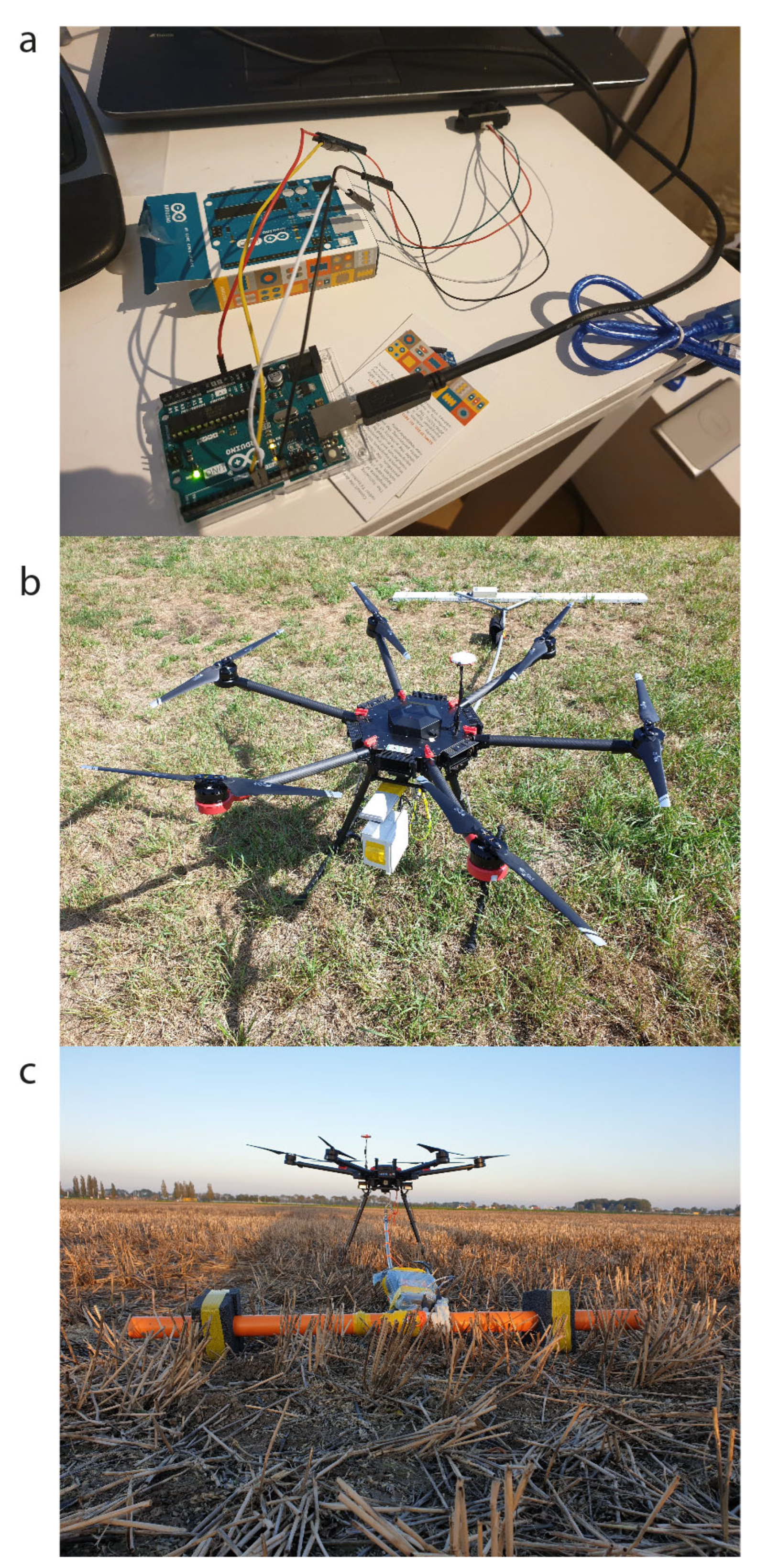
In phase 1 of our work, between 2017 and 2019, the feasibility of executing frequency domain electromagnetic surveys using affordable drones, which can carry a payload of 5 kg, was investigated (TRL level 3). Trial tests in 2017 using an off-the-shelf Geophex GEM-2 FDEM system towed on a custom-made Deltares drone showed that qualitatively acceptable FDEM data could be obtained rather easily (Figure 1a). However, several problems with respect to drone–instrument interference; safety of lift-off and landing; stable altitude flying; and the importance of accurate calibration, filtering, and altitude corrections were identified and recommended for further study. Figure 1a shows the apparent resistivity data (raw data) obtained with the GEM-2 at 8225 Hz mounted on the Deltares drone to test mapping capabilities during the flight test. In this step, we observed that the EM system was stable, and the pilot could always maintain control. Still, there were many unresolved issues, which we identified during the test flight. The most profound is the altitude control and the distance of the drone from the EM system. Those effects are illustrated in Figure 1b, where a more detailed instrument–drone separation test dataset is shown, which was later acquired using a DualEM instrument operating at 9 kHz and two coil separations at 2.0 m and 2.1 m (see Section 1 for further instrumental details). During various tests, the DualEM sensor was continuously recording and kept at a constant position, at 10 cm height, with the help of wooden blocks, and the position and activities of the drone were varied. The following sequence of recordings summarizes those main issues:

• From 0 to 600 s: recording without drone in the vicinity. Noise at about 250 s originates from users walking nearby with various clothes, smartphones, keys, etc.
• From 600 to 850 s: drone with engine off (no current) placed on top of the DualEM system.
• From 850 to 1200 s: drone with engine on stationary, placed on top of the DualEM system; Bluetooth connection of DualEM system and logger started.
• From 1200 to 1400 s: drone engines at full power on top of the DualEM system.
• From 1400 to 1450 s: drone taking off and flying fast to an altitude of several meters (no record of the exact value).
• From 1450 to 2100 s: drone flying at various heights (25, 35, 45, 55, 65, 75 cm) above the DualEM system.
• From 2100 to 2300 s: drone landed on top of the EM system; engine switched off. We observe interference, but the two frequencies have different values than before (600–800 s). We believe this is related to the drone landing with a different location and orientation with respect to the DualEM sensors than before taking off (600–800 s).
• From 2300 to 2800 s: some repetitions of the tests above. Observe the different interference after the next landing, 2650–2800 s.
• From 2800 s to end: drone was completely removed from the vicinity of the DualEM system. We observe that the values for both frequencies are the same as those at the start of the experiment.

These tests showed us that the interference from the drone is a complex matter that required further attention. It became clear that the drone needed to be separated at a sufficient distance from the EM systems to exclude any interference. The data from 2017 were not further analyzed, and we present them here as part of our first step to focus action to solve the issues.

In phase 2 in 2019 (TRL 5), the activities restarted to address the identified issues. Firstly, activities focused on safe and reliable drone-borne instrument operationalization are reported in Section 2. We discuss the preparatory tests to quantify and avoid drone–instrument interference, design a safe mounting device, optimally calibrate and correct for flight elevation variations and segment and use sounding and horizontal data. Secondly, activities focused on the data processing and interpretation scheme, as reported in Section 3.

In phase 3, also in 2019 (TRL 6), the improved and validated instrumental configurations and processing schemes were performed in three, full-scale, field validation tests which are discussed in Section 4. One validation test concerned mapping and monitoring of fresh–saline water distribution in both groundwater and surface water. The results were compared with earlier land-based geophysical data. The second field validation test considered the mapping and monitoring of sand–clay distributions near levees, relevant for seepage risk. The third field validation test was focused on the capability to detect metal cables or pipelines. The results were compared with available cone penetration tests (CPTs), borehole data and electrical conductivity measurements of surface water and groundwater.

As one can see, this work reflects our efforts from multiple scattered subprojects using various EM sensors and drones. Our initial plan could not materialize, due to sudden law changes on the payload weight, which did not allow us to fly with the Deltares custom eight-engine drone (with 15 kg payload weight, Figure 2c) with the full EM system (DualEM 842 s). Our approach can therefore be summarized in three phases:

(1)

Preliminary study to test the feasibility of flying and understand the noise level. In this phase, we used the eight-engine Deltares drone and GEM-2 system

(2)

Noise interference test, where we investigated the noise level that drones generate and performed test flights. In this phase, we used the DJI Matrice 600 and CMD MiniExplorer together with the DualEM sensors.

(3)

Data collection phase, where we utilized the DJI Matrice and CMD MiniExplorer together with the GEM-2.

2. Instrumental Principles and Tests

An FDEM instrument consists of a transmitter (TX) coil and one (or more) receiver (RX) coils. The TX coil generates a primary magnetic field (dipole) by a sinusoidal current at a discrete frequency (typically in the range of 400 Hz to 100 kHz) or multiple frequencies at once. The eddy currents induced by the primary magnetic field generate a secondary magnetic field in the subsurface that is dependent on the electrical resistivity structure of the subsurface. The secondary magnetic field alters the primary magnetic field, and the total field is captured by the receiver (RX) coil(s). The secondary field in general is very small relative to the primary field, and the total field is expressed as perturbation of the primary field in parts per million (ppm). Due to the induction process in the Earth, there is a small phase shift between the primary and secondary fields, i.e., the relative secondary magnetic field is a complex quantity with in-phase IP and quadrature Q components. The orientation of a transmitter coil is horizontal (vertical magnetic dipole (VMD)) or vertical (horizontal magnetic dipole (HMD)) and the corresponding receiver coil is oriented in a maximum coupled position, resulting in a horizontal coplanar (HCP), vertical coplanar (VCP) or perpendicular (PRP) system. By changing the transmitted frequency of the primary field and/or changing the distances between the TX and RX coils, information from different depths can be obtained.

In general, the quadrature Q ppm values of the secondary field with respect to the primary are converted to apparent resistivities, which are average resistivity values of the specific frequency and coil separation in that specific depth of investigation (McNeill, 1980). Realizing using both in-phase and quadrature data could add value, we nevertheless decided to only use apparent resistivities. To reconstruct the vertical resistivity distribution of the subsurface, a collection of apparent resistivity measurements using different frequencies/coil separations/coil orientations is gathered over an area and processed with inversion algorithms. Details about the principles and processing of EM data can be found in [15].

When combining EM sensors and drones, we are filling the gap between ground-based surveys and airborne surveys. While the goal is to avoid the complexity of an airborne survey, some issues directly related to drone-based EM systems need to be resolved, since there is no off-the-shelf system. We categorize them into four major issues:

(1)

Noise generated from the drone. In a drone survey, the limited payload capacities and engines of a drone forbid too large a separation of drone and sensors, but larger separations reduce noise.

(2)

The height of the sensor above the ground. While it is desirable to have the sensors as close as possible to the ground (typically in the order of 10–20 cm), this is considered not safe for flying.

(3)

The height of the sensors always needs to be known. Small variations in altitude during the flight generate significant artifacts in the data. In order to correct and process the data accurately, the height of the drone above the ground always needs to be known accurately.

(4)

Mounting the EM sensors to any drone while enabling it to fly smoothly and take off or land safely.

2.1. Noise Interference

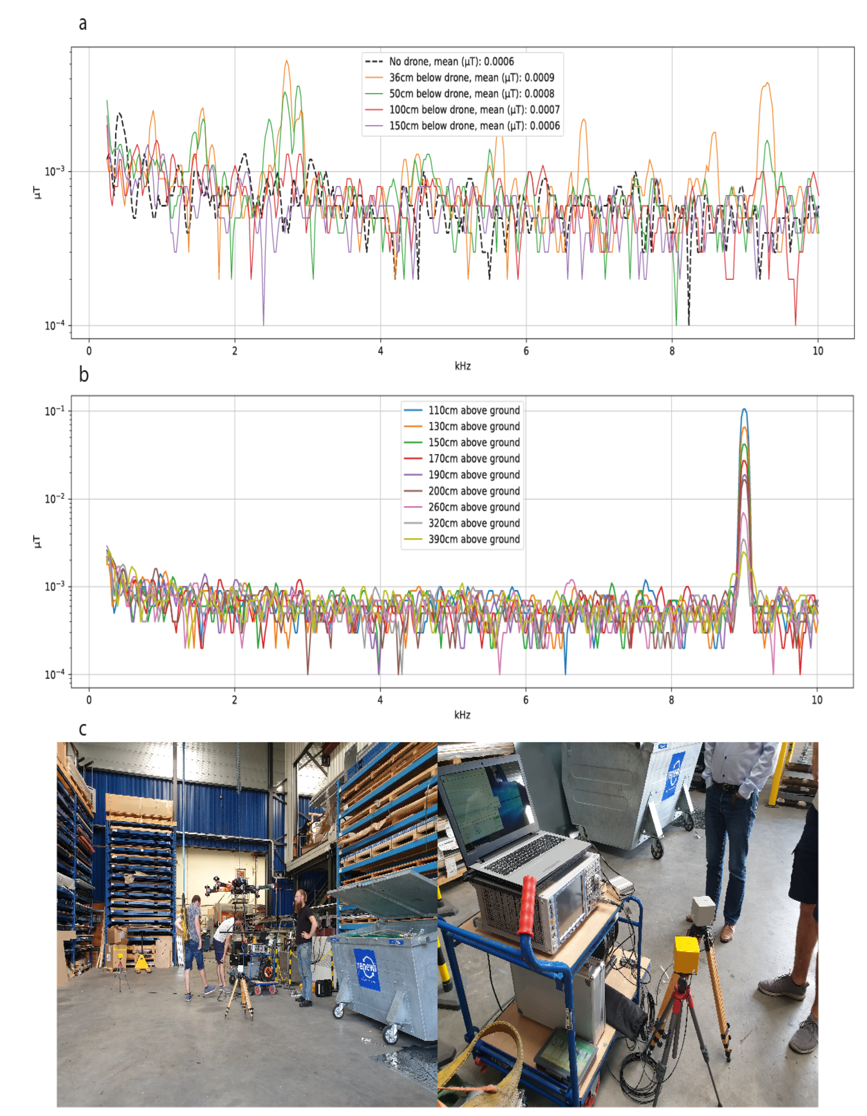
Electromagnetic interference tests were carried out by Holland Shielding systems using broadband EMF detection equipment (1 Hz–400 kHz) (Figure 2c) to determine the minimum distance between a drone and FDEM instruments and height above the ground to ensure reliable and useful data recording. The components selected and tested for interference were the following:

• Small (for geophysical applications) Deltares-developed eight-engine drones, including Global Position System (GPS) location and barometric altitude recordings.
• The 4 kg multi-coil CMD MiniExplorer (GF Instruments) that operates at 30 kHz and records with three receiver coils (at 32 cm, 71 cm and 118 cm). This tool is best suited for high-resolution near-surface investigations (up to 2 m depth).
• The 5 kg multifrequency GEM-2 that operates in a range of frequencies with one coil separation. This tool is best suited for applications deeper than 2 m and theoretically up to 15 m or more, based on the technical specifications. In most applications though, the real depth is limited to less than 10 m.
• The 28 kg DualEM 842 s that operates at 9 kHz and records with 6 coils (2.0 m, 2.1 m, 4.0 m, 4.1 m, 8.0 m and 8.1 m). This tool is also suited for deep operation (theoretically up to 13 m). In practice, the real depth of investigation is also less than 10 m.

It is common practice during surveys to avoid EM noise such as powerlines, fences and buried metallic pipes or vehicles in the vicinity. Even small metallic objects the operator could carry, such as safety shoes, mobile phones and belts, are best to be avoided during operation. Therefore, care must always be taken during the operation of an EM survey to eliminate the effect of sources, especially in the case of surveys using drones, as the drone typically has six or more electrical power engines, a carbon fiber frame and several metallic parts. In other words, it is an EM noise source itself. At the same time, the EM sensor cannot—for flight stability and safety reasons—be too distant from the drone itself.

The scope of the tests was to record the noise generated by the Deltares-developed drone and the engines in various scenarios (i.e., engine off, engine idle, engine in full power). Several components were from DJI, and thus we anticipated that commercially available drones (such as the DJI Matrice 600) would have similar behavior. The measurements were recorded with the Narda EHP-50F EMF measuring coil at a fixed location while varying the separation of the drone from the EMF coil. Figure 2a shows the results from 0.1 Hz to 10 kHz when recording without a drone (dashed black line) and a drone with engines at 36, 50, 100 and 150 cm distances from the ground (orange, green, red, and purple lines, respectively). Notice the Narda EMF sensors are held on a 30 cm base. As expected, when the separation is small (36 and 50 cm) we observe the highest mean value of noise (in the order of 8–9 × 10⁻⁴ μΤ), with some spikes well above 10⁻³ μΤ. Please note the spike at 9 kHz, the typical frequency of ground-based electromagnetic instruments. Larger separations (100 and 150 cm) show a decrease in the mean noise level; in particular, beyond a separation of 150 cm, the mean noise level is at the level of the background noise. Therefore, we decided that the separation of the drone from the sensor of electromagnetic instruments should be at least 150 cm to minimize the noise generated by the drone while at the same time having a strong primary field from the EM source.

2.2. Height above the Ground

In an EM survey, it is desirable for EM sensors to be close to the ground, although the desirable height also depends on the application. Typically, the EM sensors are held in a range of 10–100 cm above the ground, with near-surface soil investigations being in the range of 10–20 cm. Keeping that low altitude of the sensor above the ground while flying the drone is hardly possible for safety reasons. Drone pilots advised us that flying altitude, i.e., the distance of the sensor to the ground, should be in the range of 50–150 cm for safety. Considering that most ground-based EM instruments are optimized for that range and that the power of the induced EM field is limited, we investigated the strength of the responses, at different altitudes of the sensors, by elevating the instruments using a Clark device extended with wooden poles. Since most EM systems are usually designed to operate at heights of up to 1 m (human waist) we only tested heights above that. During this test, we only utilized the GF MiniExplorer in combination with the broadband EMF sensors from Holland Shielding, which were placed in a fixed position 30 cm above the ground (thus, distance from the sensor is 70 cm). No drone was present. Figure 2b shows the spectrum of the generated EM field in a range of frequencies between 0.1 Hz and 10 kHz. As expected, we observe a clear spike at 9 kHz, the operation frequency of the GF MiniExplorer. We observe a decrease in the strength of the signal with the increase in sensor separation. As mentioned, the average noise is in the order of 8–9 × 10⁻⁴ μΤ. We considered that the signal-to-noise ratio should be at least 100 times larger, and thus heights above 130 cm did not fully meet the criteria. We concluded that for the instruments selected, the optimal height above the ground, while maintaining flying safety, is in the range of 50–130 cm. The tests were also repeated with the drone at a few meters distance, resulting in the same observations and conclusions.

2.3. Analyzing Sounding Data, Calibration and Elevation Corrections

Flight elevation above the ground has a conductivity-decreasing effect on instrument readings for low-induction-number measuring methods [16]. Thus, it is of paramount importance to be able to quantify this effect using light detection and ranging (LiDAR) altitude data as well as the DEM model.

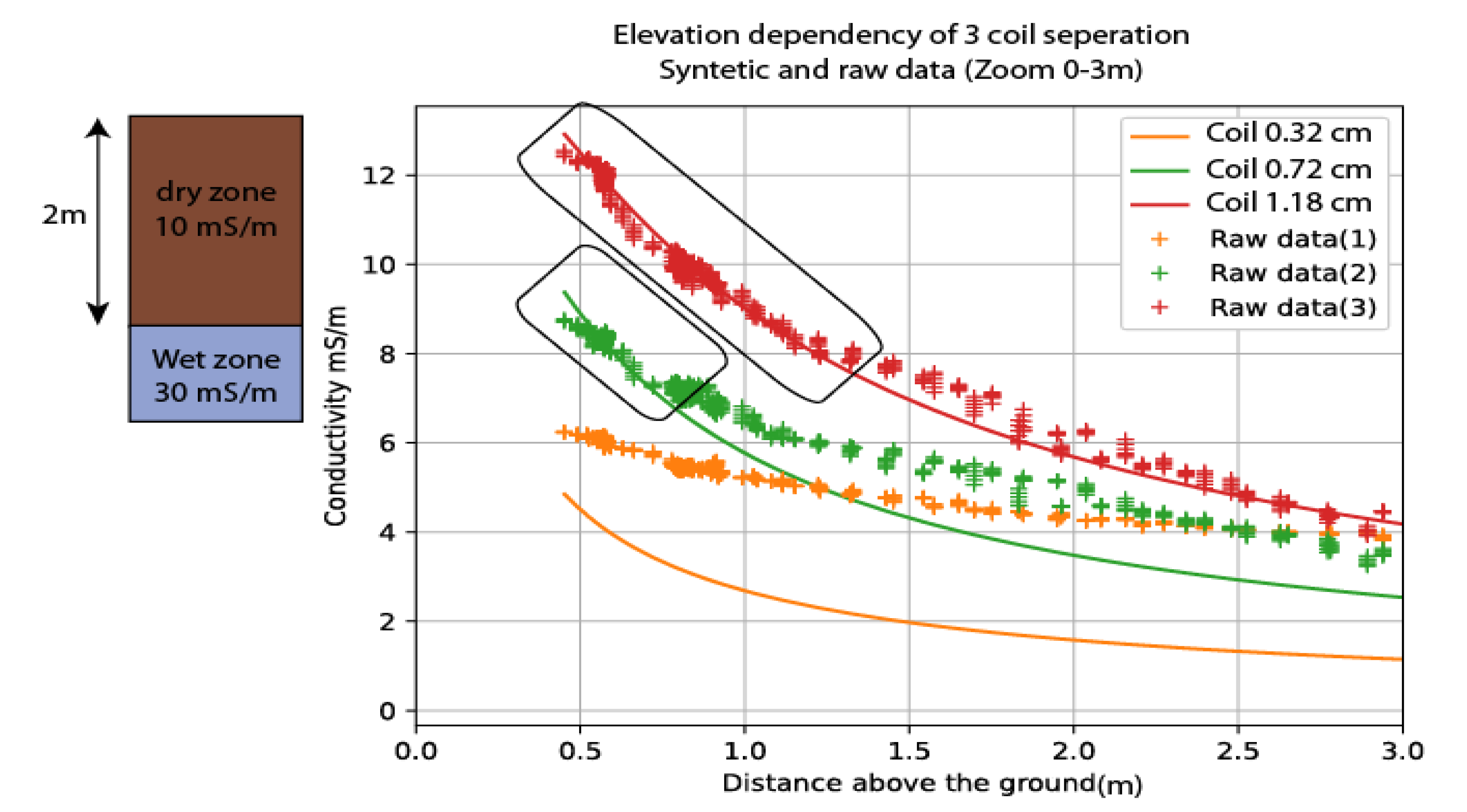
Based on the frequency, coil separation and the expected resistivity structure, it is important to estimate the usable altitude range in a process described by [16]. In our framework, we calibrate the measured data above ground with known properties, a two-layer sand zone, with a water table at 2 m depth. Figure 3 shows the raw data (scatter points) and synthetic data (continuous curves) for the CMD MiniExplorer, for different heights of the instrument. This graph shows with orthogonality the useful altitude range for the coil separations of 0.71 m and 1.18 m. The small coil separation deviates too much from the theoretical curve, and all measures were excluded from further analysis. In this graph, we proposed that the flight altitude should be no more than 0.7 m to have useful data from the two coils. Data that do not fulfill those criteria are excluded from further analysis. If the exact ground conditions are not known, it is advisable to use an averaged expected model of the area. It is worth mentioning that the CMD MiniExplorer is meant to be carried 20 cm above the ground, a height we did not test due to the flight limitations, making this small coil separation not suitable for drone flights. This is due to the thickness of the air layer between the CMD and the ground being much thicker than that expected in the intended use of the system, and for the small separation, only the air layer is sensed. In other words, as we discuss in the next section, the actual elevation is an important parameter that cannot be ignored.

As can be seen in the graph, it appears that instrumental calibration (for zero conductivity) is set at 2–3 mS/m. We collected data from higher altitudes up to 12 m, and the coil response never reached zero. We are not aware of the cause of this behavior. As mentioned, some systems allow zero-offset calibration, a practice that should be applied before each survey.

2.4. Elevation Effect on the Data

In a typical ground-based EM survey, the height of the instrument remains constant and easily controllable, as a user typically walks at a slow pace and keeps the instrument at a constant height. During the drone-based survey though, wind speed, obstacles and multiple take-offs and landings result in a variable flight elevation. Even though modern drones can automatically maintain constant height, this function is only allowed when flying above 20 m meters (according to DJI operational manual). Thus, the pilot flies in manual mode, and micro-adjustments of the height are constantly needed.

Figure 4 shows the raw recorded data (conductivity in mS/m) in a test flight for about 120 m survey length, using a CMD MiniExplorer and the DJI Matrice 600 drone. During this experiment, we flew at a constant height, increased the altitude of the drone at one location, made micro-adjustments in the altitude, and finally landed the drone. As expected, the relation between the raw measurements and height is significant. Besides the extremes (very high elevation or landing), we can see that even small elevation corrections at about 1610 m and 1680 m alter the data. Notice that in Figure 4 we show the drone height as measured by the built-in barometric sensor: the EM sensor height is below 2.5 (the pole length plus drone size). Additionally, we noted that the digital elevation model (DEM), AHN3 with 50 cm resolution from [17], and the barometric altitude show inconsistencies. The barometric altitude is valid for short periods of time and only when the weather remains constant. Therefore, it cannot be used to find the actual height accurately.

Thus, it is essential to know the height above ground of the instruments at all times. To cope with this, we developed a cheap Arduino-based LiDAR (TFmini-S) that has an operational range of 0.1 to 12 m and an accuracy of 6 cm. Additionally, to keep a timestamp of the measures, we added on the Arduino board a GPS model (Neo-6M) and an SD card module, where positioning, time and LiDAR measure are measured every second. We used the NEO-6M GPS only as a timestamp, to time-synchronize the LiDAR measures and drone positioning; thus, accuracy is of no importance. The cost of the Arduino-based LiDAR with all the components is roughly EUR 70, and it weighs around 100 g, including the protective case (see Figure 5a,b).

2.5. EM Instrument Calibration

The electromagnetic instruments of Geophex and GF Instruments are calibrated by the factory by measurements at high altitudes away from any conductive materials. However, due to conditions of the testing and field environment such as temperature or the DR-EM configuration itself, a recalibration of the instrument or a correction of the measured data is required. A procedure as described for helicopter electromagnetic surveys [15] was applied. The calibration for the data was determined by flying at a very high altitude (10 times the skin depth, >40 m). Note that some instruments (i.e., GEM-2) allow a zero-drift calibration with ferrite. Ferrite is placed on top of the RX coil and two recordings are made, one at a low altitude and one at a high altitude. If the instrument allows such calibration, it is advisable to perform it regularly or before any survey.

2.6. Mounting on the Drone and Flying

As mentioned in Section 2.1, it is best practice to have a safe distance of at least 150 cm in order to minimize the effect of the drone-generated noise. A two-axial two-meter mounting device and a 2 m long PVC-based pole were designed (see Figure 5c), limiting the instrumental rotational motion and thereby decreasing noise and increasing data quality compared to towed mounting and allowing safe lift-off, flying and sideways landing. Lastly, the pilot needed to be trained for safety assurance, and an effective drone battery change and reload procedure was developed to ensure full 8 h days of continuous DR-EM flight and recording.

2.7. Other Sources of Noise

DR-EM survey field procedures are identical to those of every land-based EM survey, excluding conditions that make flight unstable. If wind conditions allow a stable and safe flight, then DR-EM surveys follow the same steps as land-based EM surveys.

3. Data Integration, Processing and Inversion Principles and Methods Applied

In this section, we describe the steps we developed for processing the DR-EM data.

3.1. Data Integration

Before any interpretation or inversion can be executed, all measured data have to be organized. This includes integration of drone, LiDAR and electromagnetic data sources before data can be enhanced by filtering and recalibration and optionally an altitude correction of the electromagnetic profiling data. The data selection and integration are described below.

The raw data acquired in one flight are data coming from three different components of the drone-mounted electromagnetic system:

(1)

GPS time and location (Lat-Lon) and barometric altitude (bar, m) of DJI Matrice drone;

(2)

GPS time (s), location (Lat-Lon), altitude (m) and in-phase (ppm) I, quadrature (ppm) Q, resistivity (Ohm.m) or conductivity (mS/m) of each frequency;

(3)

LiDAR elevation of the altitude sensor combined with the built-in GPS.

The data are synchronized using GPS time and integrated into one raw dataset with consistent positional coordinates ready for further processing and interpretation. If the EM instrument provides I and Q values, it is best to use those values instead of resistivity or conductivity, since the altitude can be directly linked to the inversion process (airborne module) [17]. In our case, resistivity values were used (ground-based meter module) [17], and these values must be corrected for the actual height in a post-processing step. This requires a back transformation of I and Q from the exported height, with the use of the inverse Hankel transform [18,19,20]. Thus, it is important for the effect on the height to be thoroughly considered.

During the study, it soon became clear that very large quantities of data are recorded in a field survey. Typically, for every 5–10 cm of flight, over 10 parameters are recorded and processed, or in one hour, one collects 4 km and thus more than 40.000 data points, requiring proper file management. A semi-automatic processing toolbox for this and following processing steps is therefore highly recommended.

3.2. High-Frequency Noise Filtering

The data from the GEM system are already smoothed in the instrument by a low-pass filter to remove high-frequency noise. It is important to record with sufficiently high rates to capture anomalies. The raw data recordings of the CMD MiniExplorer might suffer from higher frequency noise. In the test, most sensors did not show much noise, except for the lower frequency sensors of the GEM-2. As stated in [21], applying a moving average filter is the right remedy.

3.3. Data Segmentation

The raw datasets are manually segmented into useless data, useful profile or grid data and vertical sounding data. The drone-mounted electromagnetic sensors measure continuously in a flight. The recorded data of lift-off and landing, as well as data recorded when the drone takes sharp curves at the end of a grid line and is not stable enough, are not useful. Some of the newer EM instruments record tilt and roll auxiliary data that can be used to correlate noise originating from instabilities during the flight. It is best to remove these unnecessary, often noisy, data.

The acquired data can now be split into data segments for 1D vertical electromagnetic soundings and for 2D profile and 3D grid inversion of horizontal profiling and grids.

The horizontal profile or grid segments can be split by deconvolution into two datasets:

• Datasets focusing on anomalies, caused by buried cables, pipelines, fences or metallic objects. These datasets are best analyzed with the in-phase and quadrature data.
• The overall electromagnetic response of laterally smoothly varying apparent conductivity of geological lithologies and groundwater quality are best analyzed by the procedures presented in Section 3.1.

This segmentation procedure results in sounding datasets, 2D/3D resistivity datasets and 2D/3D I/Q datasets.

3.4. Inversion and Interpretation

Inversion tries to find a model that explains the data sufficiently; i.e., synthetic data belonging to a specific resistivity model are compared with field data (apparent resistivities or in-phase quadrature). From the differences between field and synthetic data, corrections are derived and the model is updated iteratively, which is a nonlinear step. The goal of the nonlinear inversion least-squares algorithm is to recover the distribution of electrical resistivity with depth beneath each sounding. Since the data are a collation of multiple 1D measurements, data can be processed as 2D or 3D, depending on the flight paths. There are several options for inverting DR-EM apparent resistivity data, following helicopter EM (HEM) flowcharts. We chose the following ones: layered constrained inversion (LCI) if data are collected along 2D profiles [22] and spatially constrained inversion (SCI) if data are collected in grid surveys [23]. For inversion details, see the references below. In this work, we did not invert the data for anomaly interpretation (i.e., the burial depth), but only applied a qualitative analysis.

The entire flowchart of the processing of drone-borne electromagnetic survey datasets, which was applied, is shown in Figure 6. It consists of a step approach, similar to a helicopter-borne FDEM scheme published earlier [15].

3.5. Quantitative Field Data Validation

Validation of EM data and the quality of the produced inversion results is a challenge with no unique approach. In general, if all possible sources of noise that can affect the data are eliminated, the validation should be based on an independent dataset. Since resistivity is mostly sensitive to the water within the pores of the soil, the expected water level and water quality in the region can be very useful to constrain the invasions. In many cases, information about the water quality is not known, and thus the first stage of the validation is based on the existing geological maps. Even though there is no direct relation of resistivity values and geology, in a general sense, differences between sand and clay and between soil and hard rock are easily identified. If geological boreholes are present around the investigation site, then information with depth can also be obtained. Naturally, any other type of geophysical data available in the region can be used to validate the results. In the absence of any source of other datasets, then users can consider hand drilling in selected spots to investigate the soil nature and make estimations about the humidity in the ground.

Overall, the application of a DR-EM survey in the field follows the exact same conditions as a land-based EM survey, minus weather conditions affecting the stability of the flight. In other words, if the depth of investigation and the goal of the investigation can be achieved with a land-based EM system, then a drone application is also suitable. Users of DR-EM systems should base their field surveys on the suitability of the EM methods for their goal, excluding conditions forbidding the flying of drones. We believe that following this chart, the data processing has reached TRL 7.

4. Examples

Three areas were selected for DR-EM field testing:

-

A fresh–saline groundwater location grid in one of the polders near Gouda;

-

A lithological heterogeneity location profile along the levees at Vianen;

-

A cable and pipeline location near Vianen.

The coordinates used for all examples are the Amersfoort RD-new coordinates, and elevation refers to NAP (Normaal Amsterdams Peil (Amsterdam Ordnance Datum)) in meters. The flight height for all cases (i.e., the distance of the EM sensor to the ground) was in the range of 50 cm to 120 cm, as measured by the LiDAR (mean value 70 cm). In this work, we do not discuss the interpretation extensively, as this work intends to prove reliable and interpretable DR-EM data can be obtained.

4.1. Fresh–Saline Water Validation Test (Data Reported in Resistivities)

The drone-borne electromagnetic system (CMD MiniExplorer with DJI Matrice 600) was validated by executing a survey in 2020 over a known site where saline groundwater seepage occurs in a low-lying polder close to Gouda, in the Netherlands. Hydrogeological, salinity and geophysical (ERT and EM) data have been published before [24] and were available as a reference. The survey was manually flown in 4 h and resulted in a clear 3D resistivity model of the area, as shown in Figure 7.

The interpretation is as follows: Partially saturated and unsaturated zones have resistivity values of 80–250 Ohm.m (yellow to red), saline (ground)water resistivity values are <4 Ohm.m (blue), brackish groundwater has resistivity values of 10–20 Ohm.m (green, indicating total dissolved solids (TDS) of 13,000 mg/L given a formation factor of 4.1), and soil with groundwater resistivity values between 30 and 80 Ohm.m (green to yellow, indicating TDS of 3000 mg/L given a formation factor of 4.1) [25]. It is clearly visible in the data that the saline groundwater flows towards the surface in the low-lying polder. Around the polder, a levee and the higher-situated canal contain the relatively fresh polder water which was drained from the area. A ground-based EM survey was executed in 2019. During that survey, we recorded measurements using DualEM systems with 2.0 and 2.1 TX-RX separations, floating on the ditch. The scope of that survey was to measure the water salinity in ditches, and thus the depth of investigation was set to match the water depth. The results from the 2019 survey show that between the two ditches in the polder areas (the red survey lines), the north ditch shows saltier water than the south ditch. The same behavior was also observed with the drone survey, where in that case the water in the north ditch was saltier with the presence of a thin freshwater layer. The 2019 survey data are shown in Figure 7 as validation of the high contrast in the water salinities observed in the area, and that saltwater originates from the north.

The reproducibility of the data is perfect, also proven by comparing several flight path crossings. The survey speed is estimated to be 2–4 times that of an FDEM ground survey because no time is lost in crossing ditches, fences or canals. The survey duration depends very much on the logistics of drone battery management as drone batteries run out every half an hour, and the survey requires a battery charging station at hand. We were able to fly almost continuously for half a day, resulting in 7.3 km of data, four vertical soundings and six complete battery replacements. We conclude that the approach adds value in mapping fresh–saline (ground)water under these conditions.

4.2. Sand–Clay Lithology Validation Test (Data Reported in Resistivities)

The GEM-2 system with DJI Matrice 600 was also validated by executing a survey on the Lek riverside along its southern levee at Vianen in the Netherlands (Figure 8). The levee is built on top of Holocene deposits, with a variate lithology (sand, clay and peat). Sandy sediments next to and below the levees may threaten levee stability because underflow or piping can trigger a loss of stability when river water is high. Several profiles and grids were flown in 1 day to map the Holocene shallow sediments. Figure 8 shows the topographic maps, the survey lines and the locations of boreholes [17]. Notice that most of the borehole data are on top of the levee, which acts as a public road, and DR-EM data were not allowed to be collected for safety reasons.

The grid survey was able to map low-resistivity clayey soils in a few centimeters, followed by a sandy layer with variable thickness. In various locations, the sand layer can extend to −10 m NAP, even in very nearby locations (Figure 9). Overall, the area appears very heterogeneous, and the sampling density of the boreholes is not sufficient to fully capture this phenomenon. The reproducibility of the data is good as no differences occurred at crossing lines. The interpreted lithologies along the profiles and the grids are in high agreement with available borehole and cone penetration test data, based on visual inspection. More validation might be needed to get a better grip on the uncertainties in the formation factors of different lithologies.

In this case, the survey speed is also estimated to be 2–4 times that of an FDEM ground survey. In the preparation phase, it became clear that drones cannot be applied all along the river due to flight restrictions. Therefore, we conclude that the approach adds value in mapping different lithological units.

4.3. Pipeline, Cable and Fence Crossings (Data Reported in Resistivities)

The system was also validated by executing a survey over various man-made structures, such as pipelines, cables and fences, encountered at Vianen in the Netherlands. The line objects are in or on top of the Holocene deposits with varying lithology (sand, clay and peat) containing fresh groundwater. Several profiles and one grid survey flown in the previous example showed line objects. The results are shown in Figure 10.

The typical resistivity perpendicular profile over conductive line objects shows the typical anomaly with two higher resistivity lobes around a very low resistivity value trough. These anomalies are superimposed on the typical background resistivity values. It is recommended not to use the resistivity values but to use the in-phase and quadrature data recorded to interpret the anomalies for burial depth considering the obliqueness of crossing the structure, as described for instance in [7,26]. In the grid, anomalies were crossed obliquely and clearly visible in several profiles, one shown in Figure 10.

4.4. Discussion of Results

The work executed has clearly proved that drone-borne electromagnetic (DR-EM) surveying is feasible and results in high-resolution data that are comparable to those of ground surveys and much more detailed than those that can be obtained by airborne surveys. Experiences and analysis of the followed approach give indications of the conditions under which acceptable or very good quality conductivity, in-phase and quadrature data can be obtained.

Above all, there is the need for the sound selection of an instrument matching the target depth and a flying strategy to match the needs of the target of the investigation. In addition, flexible and robust data processing tools and workflow will allow cost-effective surveying and interpretation. Under these conditions, reliable data can be obtained easily. The survey speed is estimated to be 2–4 times faster than that of an FDEM ground survey.

Instrumentally, the assemblage should be designed to exclude drone–instrument interference; include elevation data recording, e.g., by LiDAR, as described before; and allow for continuous data recording and be flexible for mounting different electromagnetic instruments, suitable for different applications. For going into the field, the following flying conditions are required: drone flying permission (no-fly zones are excluded or need additional permissions), weather conditions (dry and wind speeds less than 4 Beaufort), experienced drone-pilot (capable of safe and steady manual or automatic flying), drone-battery recharging strategy (for continuous surveying) and accessibility of the area (line of sight to the drone).

The noise levels are in the order of 8–9 × 10⁻⁴ μΤ. The accuracies of conductivity values depend on whether the low-induction-number criterion is met, and this increases for low conductivity values (<0.1 mS/m) or high resistivities (>100 Ohm.m). High-frequency noise can be removed from the data by moving average filtering. This step reduces measurement noise errors significantly. Other measurement uncertainties arise from flight elevation variations and the capacity to adequately correct for them. These measurement uncertainties vary at different locations. Flight information can help indicate areas where the largest uncertainties can be expected. The test has shown that measurement accuracies are similar to or even better than those obtained by ground surveys. A great advantage is that anomalies are better detected and covered due to the high-spatial-density data collected.

With respect to the inversion, a priori information on expected lithologies or formation factors and (ground)water depth, quality or conductivity is essential for reliable interpretation of the inversion results. By using these a priori data to calibrate and constrain the inversion solutions, reliable interpretations are produced. In the example applications, the reproducibility is good and the interpreted lithologies are in high agreement with levee infrastructure maps, cone penetration soundings and visual inspection.

Three examples show the quality and use of the data and the potential for mapping saline water seepage in coastal areas; shallow geological mapping of sand, clay and peat; and shallow geological mapping of man-made conductive pipelines. Other applications envisaged are mapping water depth, water pollution, subsurface heterogeneities, faults or cavities and man-made underground infrastructures and buried objects, such as UXOs.

5. Conclusions

The first flexible drone-borne electromagnetic (DR-EM) system was designed, configured, tested and used to acquire a combination of sounding, profile and grid data of high quality in three example locations.

The three field trials showed that the data acquisition speed is 2–4 times faster than that for comparable land surveys and that, at the same time, spatial data density is 2–4 times higher. In principle, the approach followed will technically work for any drone and FDEM instrument combination. It is especially advantageous in poorly accessible terrains. However, no-fly zones and weather conditions restrict its applicability, as for airborne EM.

Using a processing scheme, adapted from HLEM, the acquired DR-EM data in the three application cases were successfully converted into quantitively accurate data allowing for a robust data inversion and interpretation of (ground)water salinity, lithology and conductive line structures, respectively. The approach is especially interesting for efficiently detailed, high-density resistivity mapping and anomaly delineation. It also works in areas that cannot or may not be accessed by foot. Repeated DR-EM surveying will allow cost-effective monitoring, for instance, of salinization.

Overall, drone-based EM surveys are in the early stages of development, requiring a high level of user input, especially on the combination of flight data and EM data. We consider the technology readiness level (TRL) to be 3 since the hardware is not mature enough yet to be used as an out-of-the-box solution. With our proposed methodology, we believe that we bring the TRL level of the hardware to level 6; i.e., the components can be used to perform a survey. On the other hand, the proposed data processing flowchart can set the TRL level to 7. Further developments can automate many of these steps of merging datasets and different sensors, so we can achieve a TRL of 9. Yet, as more field cases are published in peer-reviewed journals and attract attention from drone and EM hardware manufacturers, we expect the TRL level will increase.