Abstract
Atmospheric refraction is one of the most significant factors that affect the geolocation accuracy of high-resolution remote sensing images. However, most of the current atmospheric refraction correction methods based on empirical data neglect the spatiotemporal variation of pressure, temperature, and humidity of the atmosphere, inevitably resulting in poor geometric positioning accuracy. Therefore, in terms of the problems mentioned above, this study proposed a spatiotemporal atmospheric refraction correction method (SARCM) based on global measured data to avoid the uncertainty of traditional empirical models. Initially, the atmosphere was stratified into 42 layers according to their pressure property, and each layer was divided into 1,042,560 grid cells with intervals of 0.25 longitude and 0.25 latitude. Then, the atmospheric refractive index of each grid in the imaging region was accurately calculated using the high-precision Ciddor formula, and the result was interpolated using three splines. Subsequently, according to the rigorous geometric positioning model, the line-of-sight of each pixel and the viewing zenith angle outside the atmosphere in WGS84 were derived to provide input for atmospheric refraction correction. Finally, the coordinates of the ground control points were corrected with the calculated atmospheric refractive index and Snell’s law. The experimental results showed that the proposed SARCM could effectively improve the positioning accuracy of the image with a large viewing zenith angle, and especially, the improvement percentage for a viewing zenith angle of 34.2426° in the x-direction was 99.5%. Moreover, the atmospheric refraction correction result of the SARCM was better than that of the primary state-of-the-art methods.
1. Introduction
Achieving high-precision geolocation of remote sensing images is of great significance in the fields of mapping, resource monitoring, disaster security, and smart city construction [1,2,3]. The main factors affecting the geolocation accuracy of conventional optical sensors include internal positioning errors (main distance calibration error, internal aberration of optical lens), external positioning errors (camera installation angle error, orbit measurement error, attitude observation error), and other errors (terrain undulation) [4,5,6,7]. However, for high-resolution remote sensing images, in addition to the core errors of conventional sensors, the geolocation errors caused by atmospheric refraction are also critical for further quantitative applications [8,9]. Therefore, it is necessary to focus on the high-precision atmospheric refraction correction method for the accurate geometric calibration of high-resolution remote sensing images.
Previously, Noerdlinger proposed that the geometric error from atmospheric refraction increases with the increase in the viewing zenith angle [10]. When viewing zenith angles of 30° and 60°, the geometric errors of atmospheric refraction reach 2.22 m and 17.85 m, respectively. For this problem, satellites with kilometer resolution, such as FY-4A, Meteosat-11, and GOES-16, directly ignore this error in their geometric processing, which is because the error from atmospheric refraction when the sensor points at the nadir is much smaller than the one-kilometer resolution. In contrast, higher-resolution satellites, such as MODIS, use a constant as the atmospheric refractive index for the whole atmosphere to provide an atmospheric refraction correction. This method, known as the single-atmosphere model refraction correction method, briefly achieves a certain degree of atmospheric refraction correction, but the final correction result has a relatively large error due to the large refractive index and the small atmosphere height.
Then, with the advent of satellites with submeter resolution, it becomes more urgent to study higher precision atmospheric refraction correction methods [9,11,12,13]. One of the keys to accurate correction is the atmospheric refractive index. To this end, researchers first analyzed the atmospheric physical quantities that affect atmospheric refraction, including the imaging wavelength, air pressure, air temperature, humidity, and CO2 content [14]. The values of these physical quantities at different altitudes are then calculated using an empirical model [9,15,16]. To calculate the atmospheric refractive index, most researchers chose the Owens formula and the Weintraub and Smith formula [13,17,18,19]. Finally, two main atmospheric refraction correction methods were developed: the double-layer atmospheric refraction correction method and the multi-layer atmospheric refraction correction method [9,12,20]. The former only considers the troposphere and stratosphere [20]. It first calculates the empirical air temperature at the latitude of the imaging area to obtain the atmospheric refractive index values at different altitudes and then uses the weighted-average method to obtain the atmospheric refractive index in the troposphere and stratosphere to achieve an atmospheric correction. This method is applied to the direct geolocation of DMC3/TripleSat Constellation 1 m resolution images [20]. The latter sets the atmospheric height as and divides the atmosphere into m layers according to the equidistant . After calculating the atmospheric refractive index of each layer, the new line-of-sight after refraction is then calculated layer by layer to perform the atmospheric refraction correction. For this method, the correction accuracy improves with an increase in the number of layers. In addition, the atmospheric altitude is also one of the important factors that affect the atmospheric refraction correction results. Two atmospheric altitudes are mainly used in current multi-layer atmospheric refraction correction methods: one is the reference standard atmospheric altitude, which is mostly set to 80–87 km, and the other is the reference top stratospheric altitude, which is set to 46–50 km [9,12]. In general, although these two methods are more accurate than the single-layer model correction methods, they only consider the empirical variation with latitude and do not consider the temporal variation of air pressure, air temperature, and humidity, which inevitably causes the deviation of the atmospheric refractive index.
To solve the problem of empirical atmospheric data, some scholars recently proposed a more accurate atmospheric refraction correction method using the global measured atmospheric physical quantity data by considering the influence of different time and space [12]. Although this method directly sets the atmospheric altitude to 50 km and ignores the refraction error of atmospheric layers exceeding 50 km, as well as the errors of the measurement data itself, it provides a new idea for the study of high-precision atmospheric refraction correction.
To address the above problems, this study proposed a spatiotemporal atmospheric refraction correction method (SARCM) based on the global atmospheric physical quantity analysis data from the National Center for Environmental Prediction (NCEP). First, the atmosphere with an altitude greater than (the atmospheric height corresponding to a barometric pressure of 0.01 mb) was recognized as a vacuum, namely, the refractive index was set as 1, and the atmosphere was stratified into 42 layers according to the air pressure. Each layer was then divided into 1,042,560 grid cells of 0.25° by 0.25°, and the atmospheric refractive index of each grid was calculated according to the high-precision Ciddor formula [21]. Next, the viewing zenith angle and the line-of-sight of each pixel were calculated based on the original rigorous geometric positioning model (see Section 2.2.3 for the principles and Section 3.2.1 for the results), which were used as inputs for the atmospheric refraction correction. Finally, the refractive indices of the different layers for the particular time and space of the observation were substituted into Snell’s law to calculate the new refractive line-of-sight, and thus, obtain the corrected ground coordinates. The experimental results showed that the method proposed in this study could effectively improve the geolocation accuracy. When the viewing zenith angle was 34.2426°, the method could correct the refraction error of 2.6452 m, which was 99.5% better than that before correction in the x-direction. In addition, compared with other classical atmospheric refraction correction methods (Section 3.2.2), this method had a more accurate atmospheric height, carefully considered the variation of the atmospheric refractive index under different spatial and temporal conditions, reduced the data processing errors, and finally, achieved higher geolocation accuracy.
In the following sections, we first introduce the proposed atmospheric refraction correction method. Then, the high-precision atmospheric refraction correction was implemented using the measured data. Finally, the correction results of the method were compared with typical methods, and conclusions are given based on the experimental results.
2. The Spatiotemporal Atmospheric Refraction Correction Method
2.1. Atmospheric Refraction Error
When a sensor does not point at the nadir, the light propagates non-linearly through the atmosphere due to refractive index fluctuations in the atmosphere. Therefore, after calculating the theoretical WGS84 coordinates of the image point according to the original co-linearity equation, there will be a positioning error, that is, the atmospheric refraction error, which is shown as in Equation (1) and Figure 1:
where is the mean Earth radius of 6371.393 km. is inconsistently calculated in different atmospheric refraction correction methods. In the refraction correction method based on the single-atmosphere model:
where
where is the viewing zenith angle, is the off-nadir angle (it consists of the roll angle, the angle between the main optical axis of the camera and the Z-axis of the body coordinate system, and the scan angle of the camera pendulum mirror), is the satellite’s orbital altitude, is 1.002904 in the single-layer atmosphere model, and the atmosphere height is 10.5 km. Since is not only affected by but also varies with the orbit height altitude, the viewing zenith angle will be used to quantitatively describe the atmospheric refraction error under different observation conditions.
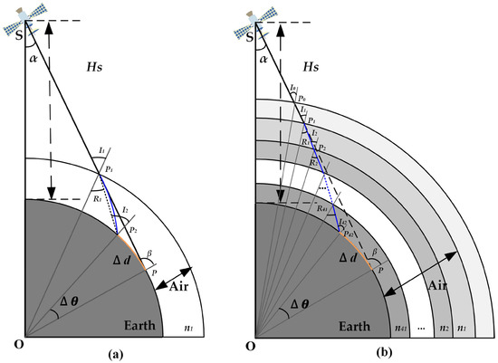
Figure 1.
Schematic of the atmospheric refraction error. (a) Atmospheric refraction error of the single-layer model. is the off-nadir angle, is the viewing zenith angle, is the satellite’s orbital altitude, is the atmospheric refraction error, and is the refractive index of the atmosphere in the model. (b) Atmospheric refraction error of the proposed model. The atmospheric refractive index value varies with time and space.
2.2. The Spatiotemporal Atmospheric Refraction Correction Method
To obtain a more accurate , this study used the pressure, temperature, humidity, and geopotential height from NCEP Global Data Assimilation System (GDAS)/Final (FNL) 0.25 Degree Global Tropospheric Analyses and Forecast Grids (083.3) to calculate the atmospheric refractive index under different atmospheric pressures and obtains the atmospheric refraction error based on the refraction line-of-sight layer-by-layer [22]. The detailed steps are as follows.
2.2.1. Calculation of the Atmospheric Refractive Index
One of the keys to achieving a high-precision atmospheric refraction correction is to calculate an accurate atmospheric refractive index. Since the refractive index fluctuates in the atmosphere, calculating an accurate atmospheric refractive index requires consideration of the effects of spatial and temporal variations. Based on previous studies, it is known that the physical quantities affecting the atmospheric refractive index mainly include the imaging wavelength, temperature, barometric pressure, humidity, and CO2 content. Among them, temperature and air pressure have significant effects on the atmospheric refractive index. In this work, two efforts were made to obtain a high-precision atmospheric refractive index: applying high-precision atmospheric refractive index formulas and using spatiotemporal atmospheric physical quantity data from the NCEP GDAS/FNL 0.25 Degree Global Tropospheric Analyses and Forecast Grids (083.3).
Regarding the former, different atmospheric refractive index formulas deal with atmospheric physical quantities differently. In 1939, Barrell and Sears first proposed a formula for the atmospheric refractive index under different meteorological conditions [14,23]:
where is the refractive index of the atmosphere under standard meteorological conditions (, , ), , is the air pressure, is the air temperature, and is the water vapor pressure. Although the accuracy of this formula for refractivity in the visible range is only , it provided a reference for later researchers to deal with atmospheric physical quantities [24,25].
Next, Elden came up with a new formula that took into account the CO2 content [14,26]. Then, Owens pointed out that Elden’s new formula still could not achieve 10−8 accuracy, and he proposed a new formula in 1967 [27]:
where
where PS and PW are the partial pressures of dry air and water vapor, respectively; is the air temperature; and is the wavelength. Many researchers are still using this formula.
In 1996, Ciddor summarized the previous research and gave a more accurate formula. Atmospheric refractivity is equal to the refractivity of dry air plus the refractivity of water vapor [21,28,29]:
where
where and are the dry air density and atmospheric refractive index that change with carbon dioxide content in the standard atmospheric environment (temperature is 15 °C, atmospheric pressure is 101,325 Pa, and relative humidity is 0%); and are the density and atmospheric refractive index of pure water vapor, respectively; and and are the dry air density and water vapor density in the current environment, which need to be calculated using the air temperature, air pressure, relative humidity, carbon dioxide content, and wavelength. The specific calculation process is given in Appendix A. This formula is relatively complex, but the accuracy of the formula for calculating the atmospheric refractive index can reach for both visible and near-infrared wavelengths [21,25].
In this article, due to the requirement for a relatively highly accurate atmospheric refractive index, we chose the Ciddor formula with an accuracy of . In addition, taking into account the present air CO2 contents, in Equation (8) was taken as 400 ppm.
Subsequently, the required data of atmospheric physical quantities, namely, air pressure, air temperature, and humidity data were also extremely important.
Most previous researchers divided the atmosphere into layers by altitude. Then, the air temperature and air pressure at different altitudes are calculated according to an empirical model, and the water vapor pressure is partially estimated using air temperature. Finally, the empirical data was substituted into the refractive index calculation formula to obtain the atmospheric refractive index values at different heights. However, the distribution of atmospheric physical quantities will change with time, altitude, and longitudes and latitudes. Therefore, the empirical atmospheric physical quantity model data cannot realize the high-precision atmospheric refraction calibration of high-resolution satellites.
To solve this problem, this work used the pressure, temperature, humidity, and geopotential height from the NCEP GDAS/FNL 0.25 Degree Global Tropospheric Analyses and Forecast Grids (083.3), which is updated every six hours and gives forecast data for the next three hours. For spatial variation, the data shows the global data of atmospheric physical quantities in the pressure range of 0.01 mb to 1000 mb, and the data is divided into 1,042,560 grid cells of 0.25° by 0.25° at each pressure value. Substituting these data into the Ciddor equation, the atmospheric refractive index of each layer could be calculated. Figure 2a shows the atmospheric refractive index when the pressure is 1000 mb in the region from 20°N to 30°N and 44°E to 54°E at noon on 1 March 2022. In practical applications, in order to obtain a more accurate spatial distribution of the atmospheric refractive index in the imaging region, cubic spline interpolation was also used here, as seen in Figure 2b. From the distribution of the atmospheric refractive index in this region, it was concluded that the atmospheric refractive index not only varied with latitude but also fluctuated in the longitude direction. Therefore, in the classical method, considering only the factor with latitude was still insufficient for the geometric refinement of high-resolution remote sensing images.
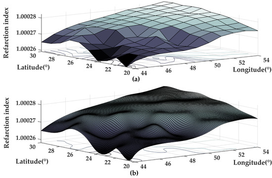
Figure 2.
Atmospheric refraction index with a pressure of 1000 mb at noon on 1 March 2022. (a) The atmospheric refraction index of the NCEP GDAS/FNL 0.25 Degree Global Tropospheric Analyses and Forecast Grids (083.3). (b) The atmospheric refraction index after cubic spline interpolation.
In addition, the swath of a satellite is often less than 400 km, that is, the longitude spanned by the imaging is often less than four longitudes. Therefore, compared with the NCEP FNL Operational Model Global Tropospheric Analyses (083.2), where each layer is divided by one longitude and one latitude, the NCEP GDAS/FNL 0.25 Degree Global Tropospheric Analyses and Forecast Grids (083.3) are more detailed.
2.2.2. Spatiotemporal Atmospheric Refraction Model
For atmospheric models, previous researchers usually stratified the atmosphere directly by altitude (single-layer atmospheric model, double-layer atmospheric model, and multi-layer atmospheric model), and then used the empirical physical quantity model data at different altitudes to calculate the atmospheric refractive index. While these models do help to correct some atmospheric refraction errors, more accurate models are needed for high-resolution remote sensing images.
Therefore, this study proposed a new atmospheric model, which stratified the atmosphere by pressure. Initially, unlike previous models that directly set a fixed value as the atmospheric height, this work treated the atmosphere above as a vacuum, namely, treating its atmospheric refractive index as 1. Subsequently, to reduce the interpolation error caused by stratification by altitude, the atmosphere was divided into 42 layers according to the air pressure since there were 41 air pressure values from 0.01 mb to 1000 mb. Additionally, each layer was composed of the 1,042,560 atmospheric refractive index grid cells calculated previously, and the cubic spline interpolation was performed in the imaging area to obtain a more detailed spatial distribution at a finer resolution. Finally, we calculated the refraction line-of-sight for each layer until the ground to achieve atmospheric refraction correction.
2.2.3. The Correction of Atmospheric Refraction Error
This work first briefly introduced the rigorous geometric positioning model converting the image point in the focal plane coordinate system to the corresponding point in the object space of WGS84. It is described by the following formula [1]:
where is the scale factor; is the principal distance of the camera; and are the offsets of the principal point in the - and -directions of the camera coordinate system, respectively; and are the distortions of the optical system in the - and -directions of the camera coordinate system, respectively; () is the coordinate of the camera projection center in the WGS84 coordinate system at the imaging time; and , , and are the rotation matrix from the camera coordinate system to the satellite body coordinate system, the satellite body coordinate system to the J2000 coordinate system, and the J2000 coordinate system to the WGS84 coordinate system, respectively.
After the rigorous geometric positioning, there are still some geometric errors that are unaccounted for, including the atmospheric refraction error. The relationship between coordinates before and after the atmospheric refraction correction is as follows:
where is the orbital inclination and is the corrected coordinate.
Figure 3 shows the flowchart of the geometric positioning with the proposed spatiotemporal atmospheric refraction correction method, and the detailed geometric process is shown in Figure 1b. The steps are as follows:
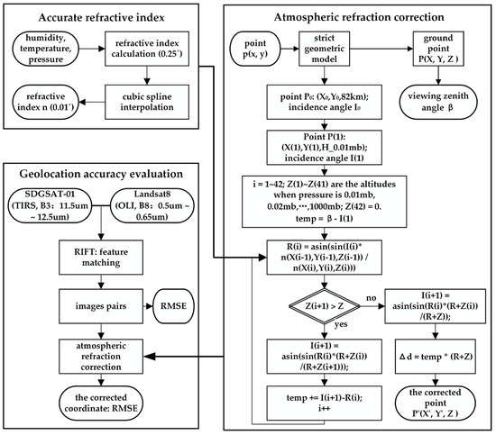
Figure 3.
Flowchart of the proposed atmospheric refraction correction method.
First, based on the rigorous geometric positioning model in Equation (9) and the SRTM30 DEM data, the line-of-sight vector of each point was calculated, and the ground control point and the point at 82 km in WGS84 were obtained. The viewing zenith angle and the were calculated:
Next, based on the geopotential height from NCEP, the atmospheric height ) at a barometric pressure of 0.01 mb was obtained so that , , , and can be calculated as follows:
Then, assuming , were the altitudes at the pressures of 0.01 mb, 0.02 mb, 0.04 mb, 0.07 mb, 0.1 mb, 0.2 mb, 0.4 mb, 0.7 mb, 1 mb, 2 mb, 3 mb, 5 mb, 7 mb, 10 mb, 15 mb, 20 mb, 30 mb, 40 mb, 50 mb, 70 mb, 100 mb, 150 mb, 200 mb, 250 mb, 300 mb, 350 mb, 400 mb, 450 mb, 500 mb, 550 mb, 600 mb, 650 mb, 700 mb, 750 mb, 800 mb, 850 mb, 900 mb, 925 mb, 950 mb, 975 mb, and 1000 mb, respectively; was equal to 0 m; from , , , , and were computed cyclically according to the following equation:
Finally, the previous step was repeated until , and then the atmospheric refraction error was calculated:
Substituting into Equation (10), the corrected coordinates of the ground control point were obtained.
2.3. Evaluation Index
Since the geometric error caused by atmospheric refraction is one of the important factors that affect the geometric positioning accuracy, this work used the geometric posi-tioning accuracy to evaluate the accuracy of the proposed spatiotemporal atmospheric refraction correction method. The root-mean-square error (RMSE) of the GCPs pairs was used as an evaluation index [30]:
where is the point of the experimental image; is the point of the reference geographic image; n is the GCPs number; and and are the components of the RMSE in the x- and y-directions in WGS84 coordinates, respectively.
3. Experiment Results and Discussion
3.1. Experiment Data
This work used the B3 (11.5–12.5 ) images of the SDGSAT-01 thermal infrared spectrometer (TIS) as the experiment images. The orbit height was 505 km, and the ground resolution was 30 m. In addition, the B8 (0.5–0.65 ) image of Landsat8 Operational Land Imager (OLI), with a 15 m ground sample distance (GSD), was used as the reference geographic image in this work. The specific parameters are shown in Table 1.

Table 1.
The main specifications of SDGSAT-01 TIS and Landsat8 OLI.
Because of the small atmospheric refraction error, when the sensor points at the nadir, the side swing images should be selected as the experimental data. Among them, the side swing angles in the emergency mode and polar mode can reach 30 and 46. In this work, the region of Saudi Arabia taken by SDGSAT-01 in emergency mode on 1 March 2022, was used as the experimental image, and the Landsat8 image taken at a similar time in this region was the reference geographic image. Then, several small 250 × 250 images were evenly selected on the experimental image, and the viewing zenith angle and geolocation of the central image point of each small image were as shown in Table 2.
Table 2.
The viewing zenith angle and the geolocation of the experiment images.
At the same time, we selected the corresponding NCEP GDAS/FNL 0.25 0.25 Degree Global Tropospheric Analyses and Forecast Grids (083.3) of the imaging time of SDGSAT-01, namely, the geopotential height, air temperature, air pressure, and relative humidity data.
3.2. Geopositioning Results of the Proposed SARCM
3.2.1. Geolocation Accuracy after the Spatiotemporal Atmospheric Refraction Correction
According to the flowchart shown in Figure 3, to evaluate the geolocation accuracy after the correction, the experimental images first needed to be feature-matched with the reference Landsat8 images using the radiation-variation insensitive feature transform (RIFT) method [31]. The accuracy of the matching using RIFT reached 0.34 pixels, and the results are shown in Figure 4. This matching accuracy and number of point pairs satisfied the computational requirements of the RMSE.
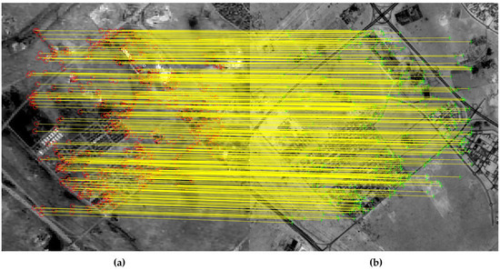
Figure 4.
Point pairs extracted with RIFT. (a) B3 image of SDGSAT-01 TIS with the original resolution of 30 m; (b) B8 image of Landsat8 OLI with the original resolution of 15 m.
Next, according to Equation (15), the geolocation accuracy of the new spatiotemporal atmospheric refraction correction method was calculated, and the results are shown in Table 3 and Table 4. Note that Table 3 is the numerical calculation of the atmospheric refraction error with different bands, while Table 4 is the geometric accuracy result of the SDGSAT-01 images with the proposed atmospheric refraction correction method.
Table 3.
Atmospheric refraction error of different bands of the proposed SARCM.
Table 4.
Geometric accuracy corrected by the proposed SARCM.
As mentioned in the previous sections, the orbital altitude, imaging wavelength, imaging time, and imaging position are the factors that affect the atmospheric refraction error. The quantitative effects of the imaging wavelength on the atmospheric refraction error are shown in Table 3. First, for the same imaging time and location, the smaller the imaging wavelength, the larger the geometric error caused by atmospheric refraction. The difference in atmospheric refraction error between different imaging wavelengths was relatively small. For example, when the viewing zenith angle was 20.1486° (34.2248° and 38.4458°), the difference between the atmospheric refraction error in the thermal and mid-wave infrared was less than 1 mm, which was much smaller than the atmospheric refraction error itself. Finally, in this work, the differences in atmospheric refraction errors between all three bands of SDGSAT-1 TIS were small enough to be negligible; therefore, only one band (11.5–12.5 μm) was used in the following to analyze the accuracy of the atmospheric refraction correction method.
From the geolocation accuracy with the same wavelength in Table 4, we obtained the following points. First, the geometric calibration after the atmospheric refraction correction with the proposed method improved the geolocation accuracy compared with the direct geometric positioning. For example, when the viewing zenith angle was 29.3865, the RMSE in the x-direction was reduced by 2.2307 m, which meant the geolocation accuracy in the x-direction was improved by 41.7% (the improvement in the x-direction was calculated using ). Next, it can be seen that the geometric error of the atmospheric refraction generally increased with the increase in the viewing zenith angle, which meant that for a large viewing zenith angle, the geometric error due to atmospheric refraction was not negligible. In addition, for the experimental images, the improvements in the geolocation accuracy with the proposed SARCM in the x-direction were significantly better than those in the y-direction. To sum up, although the GSD of the SDGSAT-1 TIS was 30 m and the geometric error in the along-orbit direction was larger than that in the across-orbit direction, the SARCM still improved the positioning accuracy to some extent. Therefore, for other higher-resolution remote sensing images, when the atmospheric refraction error becomes the main source of error after direct positioning, the positioning accuracy will be improved more obviously with the proposed method.
3.2.2. Comparison with the State-of-the-Art Atmospheric Refraction Correction Methods
Furthermore, this study selected some typical atmospheric refraction correction methods, namely, the single-layer atmospheric model (atmospheric refractive index was 1.0002904 and the atmospheric height was 10.5 km), the double-layer atmospheric model (atmospheric refractive index was from the empirical atmospheric physical quantity model data and the atmospheric height was 47.35 km), and the multi-layer atmospheric model (atmospheric refractive index was from the empirical atmospheric physical quantity model data and the atmospheric height was 84.852 km), to compare with the proposed method [9,20]. The results of geometric positioning accuracy with these methods are shown in Table 5 and Figure 5 and Figure 6. Note that Table 5 and Figure 5 show the quantitative results of different atmospheric refraction correction methods, while Figure 6 gives only the numerical calculation results of the atmospheric refraction error.
Table 5.
Comparison with the state-of-the-art atmospheric refraction correction methods.
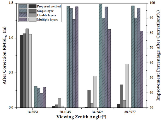
Figure 5.
Histogram of the RMSEX’ (after correction) and the improvement percentage in the x-direction of different methods.
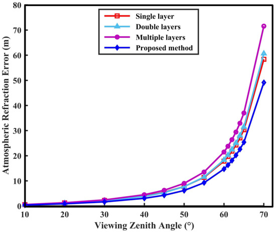
Figure 6.
Simulation results of the atmospheric refraction errors of different atmospheric refraction correction methods. The red line, light blue line, purple line, and dark blue line represent the atmospheric refraction error of the single-layer method, the double-layer method, the multi-layer method, and the proposed SARCM with different viewing zenith angles, respectively.
Table 5 shows that the RMSE values of most of the experimental images after the atmospheric refraction correction using the proposed SARCM were smaller compared with other state-of-the-art methods. In particular, in the x-direction, the geolocation accuracy after the atmospheric refraction correction using the proposed SARCM improved the most compared with the previous positioning accuracy, as shown in Table 5 and Figure 5. For example, for image 05, the geometric accuracy before the correction in the x-direction was 2.6150 m when the viewing zenith angle was 34.2406 After the correction using different atmospheric refraction correction methods, the most improvement was achieved with the proposed SARCM, which reduced the RMSE to 0.1000 m, an improvement of 99.5% compared with the original, while the least improvement was achieved with the multilayer method, which reduced the RMSE to 0.4585 m, an improvement of 82.5% compared with the original; the difference in geometric accuracy improvement between the different methods was 17%. In addition, the geometric accuracy correction in the y-direction was insignificant because the atmospheric refraction error was generated by the vertical orbit with an orbit inclination of 97.4, and the geometric error in the SDGSAT-1 TIS along-orbit direction was larger than that in the across-orbit direction.
In addition, it was found from Figure 6 that when the viewing zenith angle was small, the difference in correction results between different methods was small; however, as the viewing zenith angle increased, the correction difference between different methods also increased. For example, when the observed zenith angle was 40, the difference in atmospheric refraction error between the multi-layer model method and the proposed method was about 1 m; when the observed zenith angle was 60, the difference in atmospheric refraction error between the multi-layer model method and the proposed method was nearly 8 m. For high-resolution remote sensing images in large field-of-view imaging, the multi-layer model had relatively low geometric accuracy because it considered the influence of atmospheric refraction within the whole standard atmospheric model and its atmospheric refractive index calculated based on empirical formulas was relatively large. Further, the typical models based on empirical atmospheric physical quantity data tend to directly ignore the effects of different time and space, or just divide time by season and space by latitude to deal with the effects of different time and space, which leads to relatively low geometric accuracy for a large viewing zenith angle. However, the proposed SARCM achieved higher accuracy by considering the effects of temperature, air pressure, and atmospheric altitude changes for different times and spaces when calculating the atmospheric refractive index.
To sum up, the new method considered the spatiotemporal influence, that is, mainly the variation of temperature and pressure for different times and spaces, and thus, its accuracy was higher than the empirical methods.
4. Discussion
To improve the geometric positioning accuracy of high-resolution remote sensing images, this study not only considered the main errors of the traditional sensors but also proposed a new method to correct the geolocation errors caused by atmospheric refraction. The experimental results showed that this method could indeed further improve the geometric accuracy based on the original rigorous geometric positioning model. Moreover, the final accuracy of the proposed method in the experimental images was mostly better than that of the classical atmospheric refraction correction methods, especially in the x-direction. However, the proposed method was not always optimal in terms of the “After Correction” geometric accuracy in the y-direction. The main reason for this problem was that the atmospheric refraction error was in the across-orbit direction, and because the orbital inclination was 97.4°, the proportion of atmospheric refraction error in the x-direction to the remaining geometric error was higher than that in the y-direction on the experimental images. Therefore, the accuracy of different atmospheric refraction correction methods can be evaluated by the “After Correction” geometric accuracy in the x-direction. In contrast, because the atmospheric refraction error in the y-direction was only a small part of the remaining geometric error, it was not appropriate to evaluate the accuracy of atmospheric refraction error methods using the “After Correction” geometric accuracy in the y-direction.
In addition, although we hold the view that the accuracy of the new method was higher than the empirical methods, the NCEP GDAS/FNL 0.25 Degree Global Tropospheric Analyses and Forecast Grids (083.3) itself was also slightly biased. We can learn how to evaluate the accuracy of atmospheric physical quantities in the future. Moreover, because there are limitations in evaluating different atmospheric refraction correction methods by geometric accuracy alone when the atmospheric refraction error is small, we can learn other methods to evaluate the accuracy of the atmospheric refractive index.
5. Conclusions
With the increasingly high-resolution remote sensing sensors, a heavy price is paid when ignoring the geolocation error caused by refractive index fluctuations in the atmosphere. In this study, a spatiotemporal atmospheric refraction correction method based on global measured data of atmospheric physical quantities was proposed. This method does not set the atmosphere to a fixed height but refers to the global measured data. It directly stratifies the atmosphere according to pressure and uses the geopotential height, temperature, pressure, and relative humidity of NCEP GDAS/FNL 0.25 Degree Global Tropospheric Analyses and Forecast Grids (083.3) to compute the atmospheric refractive index for different times and spaces based on the high-precision Ciddor formula. Moreover, the line-of-sight and viewing zenith angle of each pixel was obtained according to the rigorous geometric positioning model. Finally, according to the atmospheric refraction index after the cubic spline interpolation in the image region, the corrected coordinate in WGS84 was calculated based on Snell’s law. The experimental results showed that the proposed SARCM effectively improved the positioning accuracy of the image with a large viewing zenith angle, and especially, the improvement percentage with a viewing zenith angle of 34.2426° in the x-direction was 99.5%. Moreover, the atmospheric refraction correction result of the SARCM was better than that of the primary state-of-the-art methods. Finally, applying the proposed method to the geometric processing of space-based satellites can help to realize sensitive target surveillance and disaster emergency response; if this method is used in the geometric processing of ground-based telescopes, it can also effectively improve positioning accuracy.
Author Contributions
Conceptualization, X.P. and W.H.; methodology, X.P.; software, X.P.; validation, X.L. and W.H.; formal analysis, X.P.; investigation, X.P.; resources, L.Y.; data curation, L.Y.; writing—original draft preparation, X.P.; writing—review and editing, X.P. and X.L.; visualization, X.P.; supervision, L.Y.; project administration, F.C.; funding acquisition, F.C. All authors have read and agreed to the published version of the manuscript.
Funding
This research was funded by the Strategic Priority Research Program of the Chinese Academy of Sciences under grant number XDA19010102 and the National Natural Science Foundation of China under grant number 61975222.
Data Availability Statement
Not applicable.
Acknowledgments
The authors would like to thank the SDG BIGDATA Center and National Space Science Center for providing us with data.
Conflicts of Interest
The authors declare no conflict of interest.
Appendix A
Since the geometric error caused by atmospheric refraction was considered here, only the atmospheric phase refractivity was used. The atmospheric phase refractivity is equal to the dry air phase refractivity plus the water vapor phase refractivity (ppm):
where the following factors are used:
- (1)
- The refractive index of dry air under standard atmospheric conditions (temperature of 15 °C, atmospheric pressure of 101,325 Pa, relative humidity of 0%, and CO2 content of 450 ppm) is
Correspondingly, the density of dry air in this environment is .
- (2)
- At a temperature of 20 °C and a water vapor pressure of 1333 Pa, the refractive index of pure water vapor is
Correspondingly, the water vapor density in this environment is .
- (3)
- The density of dry air in the current environment is and the density of water vapor is .
① First the density of wet air is
where is the atmospheric temperature with the unit of K, is the total atmospheric pressure with the unit of Pa, is the universal atmospheric constant with a value of , is the molar mass of water vapor with a value of , and is the molar mass of dry air:
where is the CO2 content.
The is the molar fraction of water vapor in wet air:
where the constants , and are , , and , respectively; is the atmospheric temperature with the unit of ; is the relative humidity; and the two equations for below are the saturated water vapor pressure in liquid water and on ice, respectively:
where the constants , , and are ,, , and, respectively.
is the wet air compression ratio:
where the constant values are
Each of the above atmospheric physical quantities in the formula for calculating the density of wet air can be calculated in the current environment of the atmospheric density .
② In addition, the dry air density is calculated as follows:
First, the water vapor pressure e is calculated:
From this, the dry air pressure can be calculated , and the dry air density is
③ Thus, the density of pure water vapor is:
- (4)
- Summary of the calculations:
① First, calculate the refractive index of dry air and the pure water vapor .
② According to the atmospheric CO2 content, first calculate the molar mass of dry air ; then, calculate the saturation water vapor pressure at different temperatures to calculate the molar fraction of water vapor in wet air; then, calculate the wet air compression ratio ; and substitute the previous data to calculate the density of wet air in the current atmospheric environment.
③ Calculate the water vapor pressure in the actual environment according to the saturation water vapor pressure and relative humidity h; then, calculate the dry air pressure ; then, compute the dry air density ; and finally, calculate the pure water vapor density .
④ Note: different CO2 content changes correspond to different dry and wet air density values ( and ).
⑤ Substitute into the current ambient atmospheric phase refractive index equation to obtain the desired value .
In general, the formula can be calculated with an accuracy of , but it is also relatively complex since the dry air density and pure water vapor density need to be calculated from other atmospheric physical quantity data. In addition, the CO2 content of 450 ppm proposed at the beginning of the formula was measured in a laboratory environment and is greater than the present atmospheric CO2 content, and thus, it needs to be corrected according to the current environment.
References
- Wang, M.; Cheng, Y.; Chang, X.; Jin, S.; Zhu, Y. On-orbit geometric calibration and geometric quality assessment for the high-resolution geostationary optical satellite GaoFen4. Isprs J. Photogramm. Remote Sens. 2017, 125, 63–77. [Google Scholar] [CrossRef]
- Zhang, G.; Wang, J.; Jiang, Y.; Zhou, P.; Zhao, Y.; Xu, Y. On-Orbit Geometric Calibration and Validation of Luojia 1-01 Night-Light Satellite. Remote Sens. 2019, 11, 264. [Google Scholar] [CrossRef]
- Arafat, N.; Sharawi, A.; Ragab, A. Geographic Accuracy Assessment of Geometric Corrections of World View-3 Satellite Images Using Polynomial Model (Dept. C). MEJ. Mansoura Eng. J. 2020, 45, 7–13. [Google Scholar] [CrossRef]
- Li, X.; Yang, L.; Su, X.; Hu, Z.; Chen, F. A Correction Method for Thermal Deformation Positioning Error of Geostationary Optical Payloads. IEEE Trans. Geosci. Remote Sens. 2019, 57, 7986–7994. [Google Scholar] [CrossRef]
- Wang, M.; Cheng, Y.; Tian, Y.; He, L.; Wang, Y. A New On-Orbit Geometric Self-Calibration Approach for the High-Resolution Geostationary Optical Satellite GaoFen4. IEEE J. Sel. Top. Appl. Earth Obs. Remote Sens. 2018, 11, 1670–1683. [Google Scholar] [CrossRef]
- Wang, M.; Cheng, Y.; Guo, B.; Jin, S. Parameters determination and sensor correction method based on virtual CMOS with distortion for the GaoFen6 WFV camera. ISPRS J. Photogramm. Remote Sens. 2019, 156, 51–62. [Google Scholar] [CrossRef]
- Storey, J.; Choate, M.; Lee, K. Landsat 8 Operational Land Imager On-Orbit Geometric Calibration and Performance. Remote Sens. 2014, 6, 11127–11152. [Google Scholar] [CrossRef]
- Hp, A.; Tao, H.A.; Ping, Z.B.; Zc, A. Self-calibration dense bundle adjustment of multi-view Worldview-3 basic images. ISPRS J. Photogramm. Remote Sens. 2021, 176, 127–138. [Google Scholar]
- Ye, J.; He, H.; Zhang, L.; Lin, X.; Qiang, Y. An Accurate Calculation of the Atmospheric Refraction Error of Optical Remote Sensing Images Based on the Fine-Layered Light Vector Method. IEEE J. Sel. Top. Appl. Earth Obs. Remote Sens. 2022, 15, 1514–1525. [Google Scholar] [CrossRef]
- Noerdlinger, P.D. Atmospheric refraction effects in Earth remote sensing. Isprs J. Photogramm. Remote Sens. 1999, 54, 360–373. [Google Scholar] [CrossRef]
- Schubert, A.; Jehle, M.; Small, D.; Meier, E. Influence of Atmospheric Path Delay on the Absolute Geolocation Accuracy of TerraSAR-X High-Resolution Products. IEEE Trans. Geosci. Remote Sens. 2010, 48, 751–758. [Google Scholar] [CrossRef]
- Wang, Y.; Zhu, Y.; Wang, M.; Jin, S.; Rao, Q. Atmospheric Refraction Calibration of Geometric Positioning for Optical Remote Sensing Satellite. IEEE Geosci. Remote Sens. Lett. 2020, 99, 1–5. [Google Scholar] [CrossRef]
- Wang, M.; Zhu, Y.; Wang, Y.; Cheng, Y. The Geometric Imaging Model for High-Resolution Optical Remote Sensing Satellites Considering Light Aberration and Atmospheric Refraction Errors. Photogramm. Eng. Remote Sens. 2020, 86, 373–382. [Google Scholar] [CrossRef]
- Edlén, B. The refractive index of air. Metrologia 1966, 2, 71. [Google Scholar] [CrossRef]
- Roper, L.D. Precipitation Rate versus Latitude and Longitude. 2011. Available online: http://www.roperld.com/science (accessed on 20 September 2022).
- Portland State Aerospace Society. A Quick Derivation Relating Altitude to Air pressure; Portland State Aerospace Society: Portland, OR, USA, 2004; Available online: http://psas.pdx.edu/RocketScience/PressureAltitude_Derived.pdf (accessed on 20 September 2022).
- Agbo, E.P.; Ekpo, C.M.; Edet, C.O. Trend Analysis of Meteorological Parameters, Tropospheric Refractivity, Equivalent Potential Temperature for a Pseudoadiabatic Process and Field Strength Variability, Using Mann Kendall Trend Test and Sens Estimate. arXiv 2020, arXiv:2010.04575. [Google Scholar]
- Ogunjo, S.T.; Adesiji, N.E. Statistics of vertical refractivity gradient over Akure, Nigeria. In 2020 XXXIIIrd General Assembly and Scientific Symposium of the International Union of Radio Science; IEEE: Manhattan, NY, USA, 2020; p. 4. [Google Scholar]
- Smith, E.K.; Weintraub, S. The Constants in the Equation for Atmospheric Refractive Index at Radio Frequencies. Proc. IRE 1953, 41, 1035–1037. [Google Scholar] [CrossRef]
- Yan, M.; Wang, C.; Ma, J.; Wang, Z.; Yu, B. Correction of Atmospheric Refraction Geolocation Error for High Resolution Optical Satellite Pushbroom Images. Photogramm. Eng. Remote Sens. 2016, 82, 427–435. [Google Scholar] [CrossRef]
- Ciddor, P.E. Refractive index of air: New equations for the visible and near infrared. Appl. Opt. 1996, 35, 1566–1573. [Google Scholar] [CrossRef]
- Saha, S.; Moorthi, S.; Pan, H.-L.; Wu, X.; Wang, J.; Nadiga, S.; Tripp, P.; Kistler, R.; Woollen, J.; Behringer, D.; et al. NCEP Climate Forecast System Reanalysis (CFSR) 6-hourly Products, January 1979 to December 2010. In Research Data Archive at the National Center for Atmospheric Research, Computational and Information Systems Laboratory; RDA: Boulder, CO, USA, 2010. [Google Scholar]
- Barrell, H.; Sears, J.J.E. The refraction and dispersion of air and dispersion of air for the visible spectrum. Philos. Trans. R. Soc. Lond. 1939, 238, 1–64. [Google Scholar]
- Friehe, C.A.; La Rue, J.C.; Champagne, F.H.; Gibson, C.H.; Dreyer, G.F. Effects of temperature and humidity fluctuations on the optical refractive index in the marine boundary layer. J. Opt. Soc. Am. 1975, 65, 1502–1511. [Google Scholar] [CrossRef]
- Jin, Q. Study of Factors Influencing Atmospheric Refractive Index. Master’s Thesis, Zhejiang University, Hangzhou, China, 2006. [Google Scholar]
- Edlén, B. The Dispersion of Standard Air*. J. Opt. Soc. Am. 1953, 43, 339–344. [Google Scholar] [CrossRef]
- Owens, J.C. Optical Refractive Index of Air—Dependence On Pressure Temperature and Composition. Appl. Opt. 1967, 6, 51. [Google Scholar] [CrossRef] [PubMed]
- Ciddor, P.E.; Hill, R.J. Refractive index of air. 2. Group index. Appl. Opt. 1999, 38, 1663–1667. [Google Scholar] [CrossRef] [PubMed]
- Peck, E.R.; Reeder, K. Dispersion of Air*. J. Opt. Soc. Am. 1972, 62, 958–962. [Google Scholar] [CrossRef]
- Goncalves, H.; Goncalves, J.A.; Corte-Real, L. Measures for an Objective Evaluation of the Geometric Correction Process Quality. IEEE Geosci. Remote Sens. Lett. 2009, 6, 292–296. [Google Scholar] [CrossRef]
- Li, J.; Hu, Q.; Ai, M. RIFT: Multi-Modal Image Matching Based on Radiation-Variation Insensitive Feature Transform. IEEE Trans. Image Process. 2020, 29, 3296–3310. [Google Scholar] [CrossRef]


Publisher’s Note: MDPI stays neutral with regard to jurisdictional claims in published maps and institutional affiliations. |
© 2022 by the authors. Licensee MDPI, Basel, Switzerland. This article is an open access article distributed under the terms and conditions of the Creative Commons Attribution (CC BY) license (https://creativecommons.org/licenses/by/4.0/).