TISD: A Three Bands Thermal Infrared Dataset for All Day Ship Detection in Spaceborne Imagery

Abstract

The development of infrared remote sensing technology improves the ability of night target observation, and thermal imaging systems (TIS) play a key role in the military field. Ship detection using thermal infrared (TI) remote sensing images (RSIs) has aroused great interest for fishery supervision, port management, and maritime safety. However, due to the high secrecy level of infrared data, thermal infrared ship datasets are lacking. In this paper, a new three-bands thermal infrared ship dataset (TISD) is proposed to evaluate all-day ship target detection algorithms. All images are from SDGSAT-1 satellite TIS three bands RSIs of the real world. Based on the TISD, we use the state-of-the-art algorithm as a baseline to do the following. (1) Common ship detection methods and existing ship datasets from synthetic aperture radar, visible, and infrared images are elementarily summarized. (2) The proposed standard deviation of single band, correlation coefficient of combined bands, and optimum index factor features of three-bands datasets are analyzed, respectively. Combined with the above theoretical analysis, the influence of the bands’ information input on the detection accuracy of a neural network model is explored. (3) We construct a lightweight network based on Yolov5 to reduce the number of floating-point operations, which is beneficial to reduce the inference time. (4) By utilizing up-sampling and registration pre-processing methods, TI images are fused with glimmer RSIs to verify the detection accuracy at night. In practice, the proposed datasets are expected to promote the research and application of all-day ship detection.

1. Introduction

Ship detection is of great value in marine traffic management, navigation safety supervision, fishery management, ship rescue, ocean monitoring, and other civil fields. Timely acquisition of ship location, size, heading, and speed information is of great significance to ensure maritime safety. Due to the complexity of the ocean environment, high labor cost, experience dependence, and unreliable manual observation, automatic ship detection using remote sensing images (RSIs) has attracted more and more interest.

At present, remote sensing satellite images mainly include visible, infrared, and synthetic aperture radar (SAR). With the limited number of SAR satellites and long revisiting period, the applications based on SAR images cannot achieve real-time ship monitoring. Due to the great variation of weather and wind speed, there is high non-uniformity of sea surface clutter in SAR images [1], which is not conducive to ship detection based on SAR images. Ship monitoring based on spaceborne optical images works well, except when there is heavy cloud cover and light restriction. Infrared imaging systems can record the radiation, reflection, and scattering information of the object to overcome some of the negative effects of thin clouds, mist, and dark light. Therefore, target detection based on thermal infrared remote sensing images has become one of the important means of all-day Earth observation.

Ship detection comprises hull and wake detection [2]. However, ship wakes do not always exist; therefore, hull detection is more widely used. In recent years, researchers have proposed a variety of ship detection algorithms based on RSIs. In general, ship target features are extracted by traditional or intelligent methods. Computer-assisted ship detection methods typically involve feature maps extraction and automatic location by classifiers, thereby freeing human resources. Traditional detection methods extract middle or low level features containing the color, texture, and shape of targets. Intensity distribution differences between ships and waters are helpful to distinguish ship candidates from sea, but the effectiveness varies across different sea types and states. Since the sea surface is more uniform than the target, Yang et al. [3] defined intensive metrics to distinguish anomalies from relatively similar backgrounds. Zhu et al. [4] firstly segmented images to obtain simple shapes, and then extracted shape and texture features from ship candidates. Finally, three classification strategies were used to classify ship candidates. In calm seas, the results of the above method are stable. However, the algorithm based on low-level features has poor robustness when wave, cloud, rain, fog, or reflection occur. In addition, manual feature selection is time consuming and strongly depends on the expertise of the user.

Consequently, later research has focused on how to extract and incorporate more ship features to detect ships more accurately and quickly. In recent years, convolutional neural network (CNN) has made many breakthroughs. Through a series of convolutional and pooling layers, more distinguishable features can be extracted by CNN. However, the accuracy of data-driven CNN detection methods largely depends on large-scale and high-quality training datasets. Driven by CNN, intelligent methods based on advanced features are mainly divided into two categories. The two-stage algorithms first utilize the region proposal network to select the approximate objects region, and then the target detection network classifies the candidate region to obtain more accurate boundaries. Two-stage models mainly contain R-CNN [5], Fast R-CNN [6], and Faster R-CNN [7]. The one-stage detection methods include SSD [8], RFBNet [9], and YOLOv1 [10], YOLO9000 [11], and YOLOv3 [12]. One-stage algorithms omit the region proposal process and directly return to the bounding box and assign the relevant class probability.

The accuracy of the supervised algorithm is closely related to the quality of the datasets. Although various public datasets such as ImageNet [13], PASCAL VOC [14], COCO [15], and DOTA [16] can be used to identify multiple general targets, they are not specifically meant for ship detection. Some large remote sensing targets datasets, such as FAIR1M [17], include geographical information containing latitude, longitude, and resolution attributes to provide abundant fine-grained classification information. Qi et al. [18] designed MLRSNet datasets for multi-label scene classification and image retrieval visual recognition tasks. Zhou et al. proposed a large-scale Patternnet-Google Maps/API [19] dataset which is suitable for deep learning-based image retrieval methods. The open large datasets have greatly accelerated the development of target detection. However, public datasets specific to maritime vessel detection are still not available.

To sum up, there are three main challenges for space-based thermal infrared all-sky automatic ship detection research: (1) Due to the high security level of infrared data, training datasets of thermal infrared remote sensing images for ship detection are scarce. (2) During heat source imaging, the target and boundary may be too indistinct to distinguish, which may lead to false alarms or missed detection. (3) Due to the lack of a clear connection between network parameters and approximate mathematical functions, the interpretability of CNN is poor. The neural network can find as many ships as possible and predict the accurate target position, but it is not known which input information is useful.

In this paper, we label a new three-bands thermal infrared ship dataset (TISD) to solve the above challenges. All images are from the SDGSAT-1 thermal imaging system (TIS) real remote sensing images. SDGSAT-1 is designed for a sun-synchronous orbit at an altitude of 505 km. The SDGSAT-1 website: http://www.sdgsat.ac.cn/ (accessed on 14 October 2022). In order to describe human activities in detail, three loads of thermal infrared, glimmer, and multispectral imagers are consulted, among which, the spatial resolution of TIS is 30 m and the imaging width is 300 m. By utilizing the TISD, an advanced detector, namely the improved Yolov5s [20], is used to train the all-sky ship target detection model. Combined with data feature analysis, the influence of bands selection on target detection accuracy is evaluated. The all-day detection capability is verified with glimmer images. In practice, the proposed datasets are expected to promote the research and application of all-day ship detection. The main contributions of this paper are as follows:

• To the best of our knowledge, we are the first to annotate the three-bands thermal infrared ship dataset. All images are from the SDGSAT-1 TIS three-bands real remote sensing images. To enrich the proposed datasets, the selected images contain features of different target sizes and illumination levels in a variety of complex environments. TISD Website: https://pan.baidu.com/s/1a9_iT-pdaSZ-hkBYU2Qciw?pwd=fgcq (accessed on 14 October 2022).
• Due to the lack of clear connection between network parameters and approximate mathematical functions, it is not known which input information is useful. In order to explore the relationship between input information and detection accuracy, the optimum index factor (OIF), which is related to the key information and redundancy between different bands images, is used appropriately to evaluate the useful features in our dataset.
• Based on TISD, we used the state of art detector that we proposed before, namely, the improved Yolov5s [20], as the baseline to train different models by utilizing different spectral bands datasets. Combined with the above theoretical analysis, the influence of combined bands on detection accuracy is explored.
• The difficulties of the existing ship detection methods based on datasets are summarized. By using up-sampling and registration pre-processing methods, glimmer images are combined with thermal infrared remote sensing images to verify the all-day ship detection capability.

The organizational structure of this study is as follows. In Section 2, the related work of publicly available ship datasets is elaborated in detail. In Section 3, the description of the datasets is outlined. In Section 4, we present experiments and discuss the experimental results to validate the effectiveness of the proposed research. Finally, in Section 5, we summarize the content of this study.

2. Related Works

At present, RSIs from radar, optical, reflective infrared, and thermal infrared are mainly used for ship detection, as shown in Figure 1. As an active microwave sensor, SAR can obtain high-resolution data under various weather conditions, and has been widely used in ocean surveillance [21,22]. With the development of deep learning and imaging technology, many automatic target algorithms for RSIs have been proposed to detect different targets. To capture the features of ships with large aspect ratio, Zhao et al. [23] proposed a new attentional reception pyramid network, which has asymmetric core sizes and various dilated rates. Due to different local clutter and low signal-clutter ratio existing in SAR images, Wang et al. [24] used variance-weighted information entropy method to measure the local difference between the targets and its neighborhood. Then, the optimal window selection mechanism based on multi-scale local contrast measures are utilized to enhance the target from the complex background. Considering the difference in gray distribution and shape between ship and clutter, Ai et al. [25] modeled using the ship target’s gray correlation and joint gray intensity distribution of strong clutter pixel and its adjacent pixel in two-dimensional joint lognormal distribution, which greatly reduced the false positives caused by speckle and local background non-uniformity. Gong et al. [26] presented a novel neighborhood-based ratio operator to produce a difference image for change detection in SAR images. Zhang et al. [27] proposed an unsupervised change detection method using saliency extraction; however, this method is not suitable for object detection in a single-frame image. Song et al. [28] generated proven robust training datasets by using synthetic SAR images and automatic identification system data; however, the acquisition of the above data requires the establishment of ground base stations, which is limited by region and lacks real-time capability. Rostami et al. [29] proposed a new semi-supervised domain adaptive algorithm based on existing optical images labels to transfer features learned from optical to SAR. To be more intuitive, the existing general multi-target detection datasets with ship targets and the proposed TISD are summarized, as shown in

Table 1. The summary of ship datasets.

Images Type	Datasets	Source Satellite	Numbers	Resolution	Feature Description
SAR	OpenSARShip2.0 [30]	Sentinel-1	Collect messages from the ship chip integrated with the Automatic Identification System.	1–15 m	Data can be updated, but the sample size is uneven between categories.
	SSDD [31]	RadarSat-2, TerraSAR-X, Sentinel-1	1160 images, 2456 multi-scale ships	1–15 m	It is the first ship dataset specially for SAR images.
	AIR-SARShip2.0 [32]	Gaofen-3	300 images	1 m, 3 m	Contains harbors, islands, coral reefs, near-shore, and sea surfaces under different conditions.
	SAR-Ship-Dataset [33]	Gaofen-3, Sentinel-1	210 images	3 m, 5 m, 8 m, 10 m	Contains different sizes ships and backgrounds.
	HRSID [34]	Sentinel-1B, TerraSAR-X, TanDEM-X	5604 images, 16,951 ships	0.5 m, 1 m, 3 m	Includes SAR images of different resolutions, polarization, sea state, sea area and coastal ports.
Optical	HRSC2016 [35]	Google Earth	1070 images, 2976 instances with rotated bounding boxes	0.4–2 m	It has the advantages of rich object features and sharp shooting angle from many directions.
	HPDM-OSOD [36]	Google Earth	1127 images, 5564 instances with rotated bounding boxes	0.4–2 m	Compensate for the lack of diversity in public datasets.
	DOSR [37]	Google Earth	1066 images, 6172 ship targets	0.4–2 m	Break through the limitation of lack of datasets for fine-grained ship detection.
	DOTA-ship [16]	Google Earth, JLin-1, Gaofen-2	573 images, 43,738 instances with rotated bounding boxes	Space-based and aerial images	The distribution of ships size is unbalanced.
Video	SeaShips [38]	video from Guangdong Province, China	31,455 images	ground based images	Captured by cameras deployed in the shoreline surveillance system.
Thermal Infrared	TISD	SDGSAT-1 TIS	2190 images, 12,774 ships targets	10 m	Compensate for the lack of public space-based TI ship datasets.

The resolution of SDGSAT-1 TIS is 30 m, the images of TISD are up-sampled to 10 m.

.

As the only available fine-grained ship dataset, HRSC2016 [35] has been used as a baseline in many studies. By using public ship dataset HRSC2016, Wang et al. [39] validated an improved encoder–decoder structure which added a batch normalization (BN) processing layer to speed up model training and introduced extended convolution at different rates to fuse features of different scales. However, some subcategories of HRSC2016 contain no more than ten ship instances, and some small ships are neglected during marking. Given the lack of diversity in public datasets, Cui et al. [36] established HPDM-OSOD and proposed a novel anchor-free rotating ship detection framework, SKNet. The ship target center key points and shape dimensions, including width, height, and rotation angle, are utilized during modeling to avoid many predefined anchors in the rotating ship detector. For the limitation of fine-grained datasets, Han et al. [37] established a new twenty-class three-level directional ship recognition dataset (DOSR). Li et al. [40] combined the classic Saliency Estimation algorithm and deep CNN object detection to ensure the extraction of large ships from multi-scale ships in high-resolution RSIs. Yao et al. [41] used a region proposal regression algorithm to identify ships of panchromatic images, but the large parameters of the network led to long prediction times. Due to the large size of the remote sensing images, Zhang et al. [42] firstly utilized a support vector machine to classify the water and non-water areas. However, ships close to shore are difficult to classify by the preprocessing separation method.

As opposed to SAR or spaceborne optical images, ground-based visual images can achieve better accuracy and real-time processing for ship detection, which can be widely used in port management, cross-border ship detection, autonomous shipping, and safe navigation. Li et al. [43] introduced the attention module to the YOLOv3 network to achieve a good application for real-time ship detection in a real scenario. Shao et al. [44] used the Seaships dataset [38] to train CNN to predict the approximate position of ships, and then used significant area detection and coastline information based on global contrast to correct the position of ships. For continuous video detection tasks, accuracy should be sacrificed to ensure real-time processing.

Due to the high secrecy of the infrared remote sensing data, the supply of images is very limited; therefore, it is difficult to collect many positive samples of ships. Transfer learning is helpful when the amount of data is insufficient. Wang et al. [45] used optical panchromatic images to assist limited infrared data during auxiliary training; however, there is a great difference between infrared and panchromatic images in imaging principle. Song et al. [46] collected dark light boat images from the infrared cameras on the ships. The datasets contain 3352 marked images of a variety of ship navigation states and interference scenarios. Li et al. [47] utilized MarDCT videos and images from fixed, mobile, and pan-tilt-zoom cameras [48], as well as the PETS2016 dataset [49] for visual performance evaluation. It must be noted that the above studies are not based on real spaceborne infrared remote sensing data [50,51], and infrared RSIs have irreplaceable value in the field of ship detection. Therefore, to make up for the lack of a spaceborne thermal infrared public dataset, we notated a thermal infrared ship dataset in three bands based on SDGSAT-1 TIS images.

3. Datasets Analysis

In this paper, we propose a new dataset which consists of 2190 768 × 768 images, containing day and night, and 12,774 targets selected from a 4.23–7.53 [20] aspect ratio. All images are from SDGSAT-1 TIS three-bands RSIs of the real world. Each image in our dataset is accurately annotated using labels and bounding boxes. There are three bands in the TISD, including: B1: 11.5~12.5 µm, B2: 8~10.5 µm, and B3: 10.3~11.3 µm. To enrich the TISD, the images are selected to cover a set of features including different sizes, lightings, and scenes. The following are detailed steps for labeling the datasets and for data analysis.

3.1. Movement Correction Based on Cross Correlation Method

Different from geometrically aligning [52], the offset between different channels is horizontal and vertical in TISD. Therefore, cross-correlation program is chosen to calculate offset from different channels. The cross-correlation function represents the correlation degree between two random or deterministic signals at any two different time. It is assumed that image $f_2$ is obtained by translation of $f_1$, as shown in Equation (1), and then it is transformed according to Fourier theorem in Equation (2). The Fourier transform is computed for the cross-correlation function, as in Equations (3) and (4). Finally, Equation (4) is transformed by inverse Fourier to get Equation (5).

$$f_2=f_1(x-\mathrm{\Delta }x,y-\mathrm{\Delta }y)$$

(1)

$$F_2(u,v)=F_1(u,v)e^{-2\pi j(u\mathrm{\Delta }x+v\mathrm{\Delta }y)}$$

(2)

$$R_{ccf}(x,y)=f_1(x,y)\ast f_2(-x,-y)$$

(3)

$$R_{ccf}(u,v)=F_1(u,v)F_2^{*}(u,v)=F_1{F}_1^{*}{e}^{2\pi j(u\mathrm{\Delta }x+v\mathrm{\Delta }y)}=F(u,v)e^{2\pi j(u\mathrm{\Delta }x+v\mathrm{\Delta }y)}$$

(4)

$$R_{ccf}(x,y)=F(x,y)\ast \delta (x-\mathrm{\Delta }x,y-\mathrm{\Delta }y)=F(x-\mathrm{\Delta }x,y-\mathrm{\Delta }y)$$

(5)

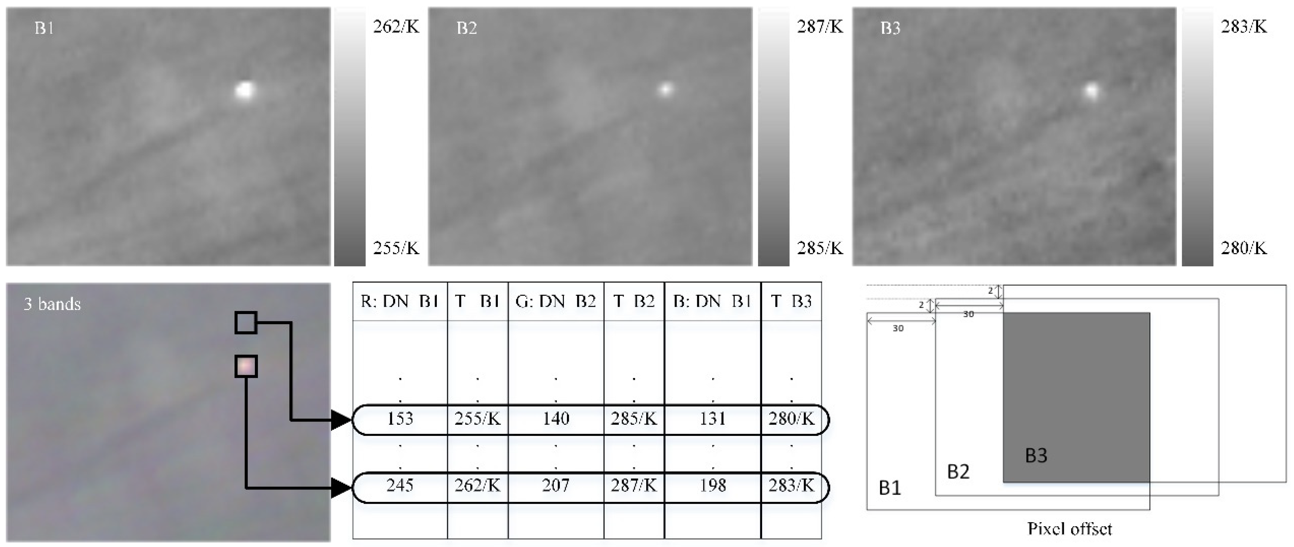
According to the cross-correlation function, the peak value of $F(x,y)$ is at the origin and the peak value of $R(x,y)$ is at the $(\mathrm{\Delta }x,\mathrm{\Delta }y)$, which is the offset of $f_2(x,y)$. The horizontal displacement deviation of image blocks with rich texture can be calculated quickly and intuitively by the cross-correlation registration method. The offsets of images with 30 m and 10 m resolutions are calculated, and the difference between normalized offsets is negligible, as shown in

Table 2. The horizontal and vertical pixel offsets of two adjacent band images.

	Resolution of 30 m		Sampling up to 10 m
$\mathrm{\Delta }{x}_{B1-B2}$	30.0078/pixel	900.234/m	91.4238/pixel	914.238/m
$\mathrm{\Delta }{x}_{B2-B3}$	30.0166/pixel	900.498/m	89.1290/pixel	891.290/m
$Mean\mathrm{\Delta }x$	30.0122/pixel	900.366/m	90.2764/pixel	902.764/m
$\mathrm{\Delta }{y}_{B1-B2}$	2.0035/pixel	60.105/m	5.8984/pixel	58.984/m
$\mathrm{\Delta }{y}_{B2-B3}$	2.0893/pixel	62.679/m	6.2266/pixel	62.266/m
$Mean\mathrm{\Delta }y$	2.0464/pixel	61.392/m	6.0625/pixel	60.625/m

. The horizontal and vertical offsets of two adjacent band images with a resolution of 30 m are 30 pixels and 2 pixels, respectively, are shown in Figure 2.

Where $\mathrm{\Delta }{x}_{B1-B2}$ is the horizontal offset of bands B1 and B2, $\mathrm{\Delta }{x}_{B2-B3}$ is the horizontal offset of bands B2 and B3, $\mathrm{\Delta }{y}_{B1-B2}$ is the vertical offset of bands B1 and B2, and $\mathrm{\Delta }{y}_{B2-B3}$ is the vertical offset of bands B2 and B3 with the resolution of 30 m or 10 m. (m represents meters).

In this paper, B1 channel is 11.5~12.5 µm, B2 channel is 8~10.5 µm, and B3 channel is 10.3~11.3 µm. After B2 translates 30 pixels to the left and B3 translates 60 pixels to the left, image fusion can be carried out after registration with B1, corresponding to the R, G, and B channels of fusion images, as shown in Figure 2.

3.2. Labeling Process

The length of aircraft carriers or cruisers is about 200–350 m, which can account for 7–12 pixels in a 30 m resolution image. However, the standard length of common marine fishing vessels is generally less than 100 m, which takes up fewer pixels. To facilitate the annotation, the image should be preprocessed by up-sampling, mainly including nearest neighbor interpolation, bilinear interpolation, and bicubic interpolation. In order to avoid sacrificing image quality, we adopted the time-consuming bicubic interpolation method, shown in Equation (6), where $S(x)$ is the interpolation kernel and $\mathrm{f}(\mathrm{M})$ is the interpolation calculation formula of pixel values of corresponding scaled matrix coordinate points, as shown in Formula (7), where A, B, and C are matrices and $\mathrm{Im}$ is the original gray matrix.

$$S(x)=\{\begin{array}{c}1-2{\left|x\right|}^2+{\left|x\right|}^3,\left|x\right|<1\\ 4-8\left|x\right|+5{\left|x\right|}^2-{\left|x\right|}^3,1\le \left|x\right|<2\\ 0,\left|x\right|\ge 2\end{array}$$

(6)

$$\mathrm{f}(\mathrm{M})=\mathrm{A}\ast \mathrm{B}\ast \mathrm{C}$$

(7)

$$\{\begin{array}{c}\mathrm{A}=\left[\mathrm{S}\right(\mathrm{u}+1),\mathrm{S}(\mathrm{u}-1),\mathrm{S}(\mathrm{u}-2\left)\right]\\ \mathrm{B}=\mathrm{Im}[i-1:i+2,j-1:j+2]\\ \mathrm{C}={[\mathrm{S}(\mathrm{v}+1),\mathrm{S}(\mathrm{v}-1),\mathrm{S}(\mathrm{v}-2)]}^{’}\end{array}$$

(8)

After registration and up-sampling, the LabelImg software is used to annotate triple-channel pseudo-color patches with a resolution of 10 m. Specifically, in PASCAL VOC XML annotation format, bndbox represents the four coordinate values in the upper left and lower right corner of the annotation box. Additionally, it should be noted that the coordinate origin is the upper left corner of the picture, as shown in Figure 3.

3.3. Statistical Analysis of Dataset

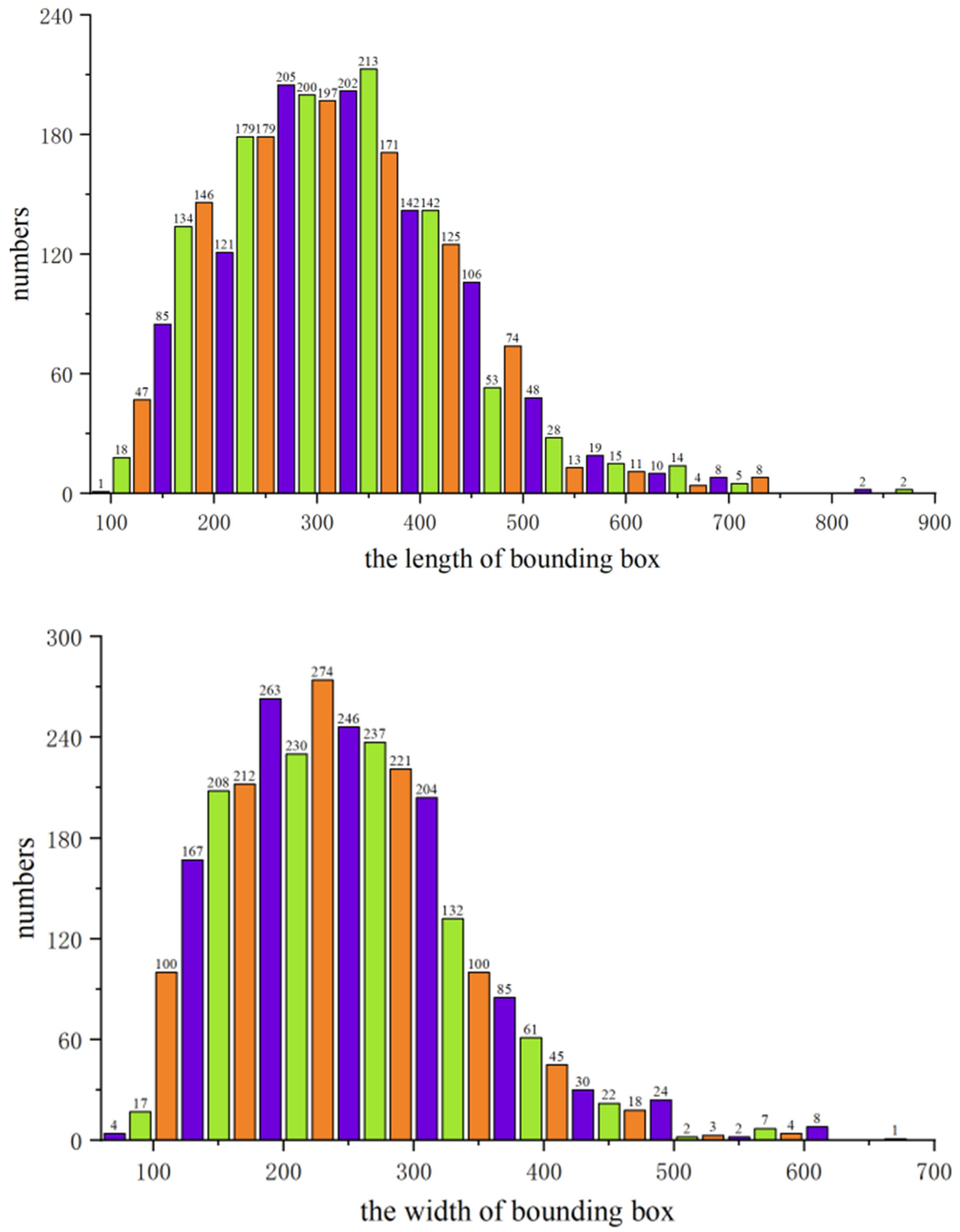
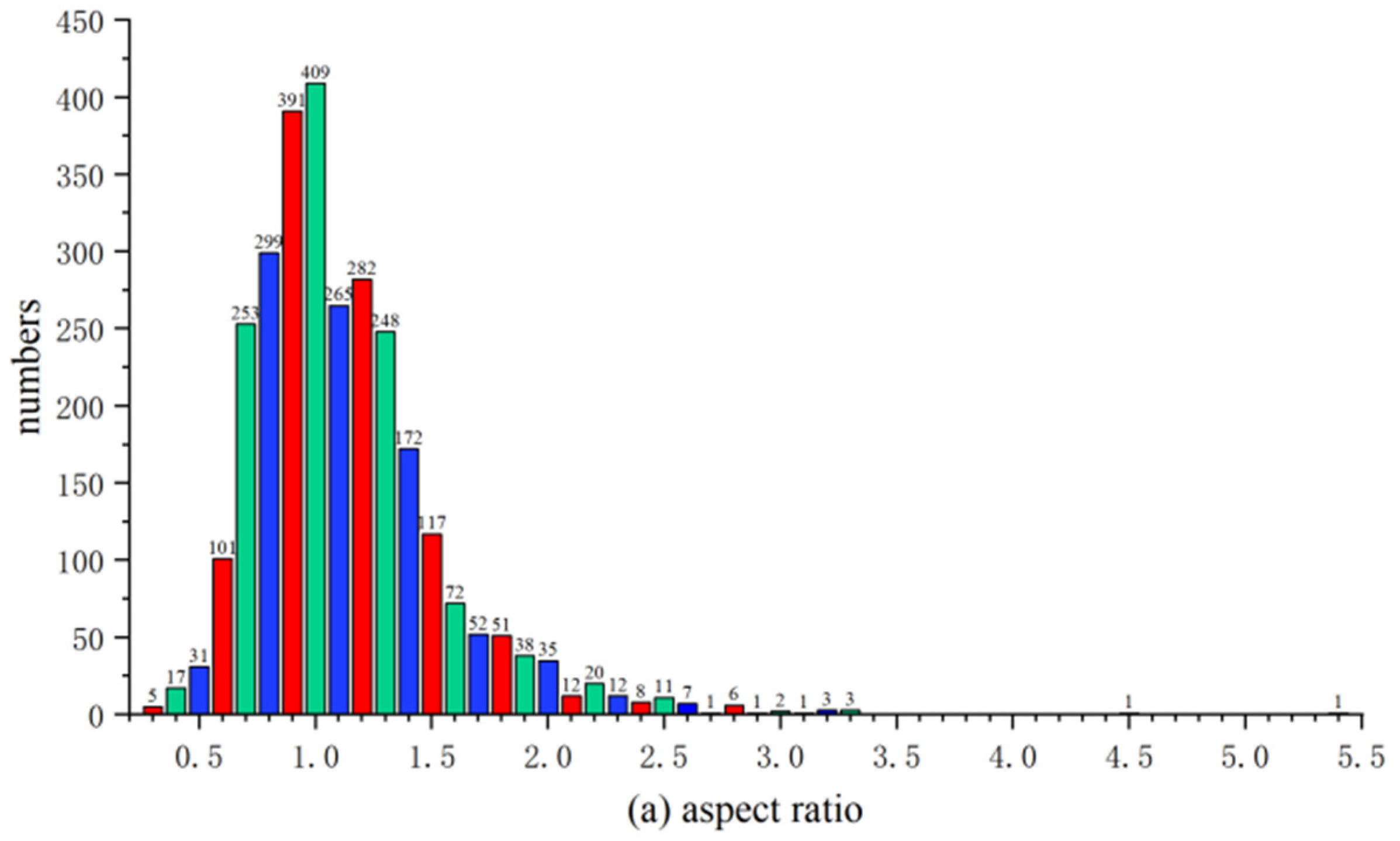
In the TISD, band B1 contains 545 images and 2927 ships, with an average of 5.37 ships per image. After statistical analysis of the target bounding boxes, the length of anchor boxes is 9 to 87 pixels, namely 90 to 870 m in the image with 10 m resolution. The width of an anchor box includes 7 to 67 pixels, that is, 70 to 670 m in the image with 10 m resolution, as shown in Figure 4. The aspect ratio in the TISD is widely distributed, mainly from 0.3 to 3.5, as shown in Figure 5. In the process of designing potential target area, candidate boxes of different sizes and aspect ratios have been weighed. The TISD contains a minimum temperature difference of 0.3226 K between that of ship and sea.

3.4. Dataset Feature Analysis

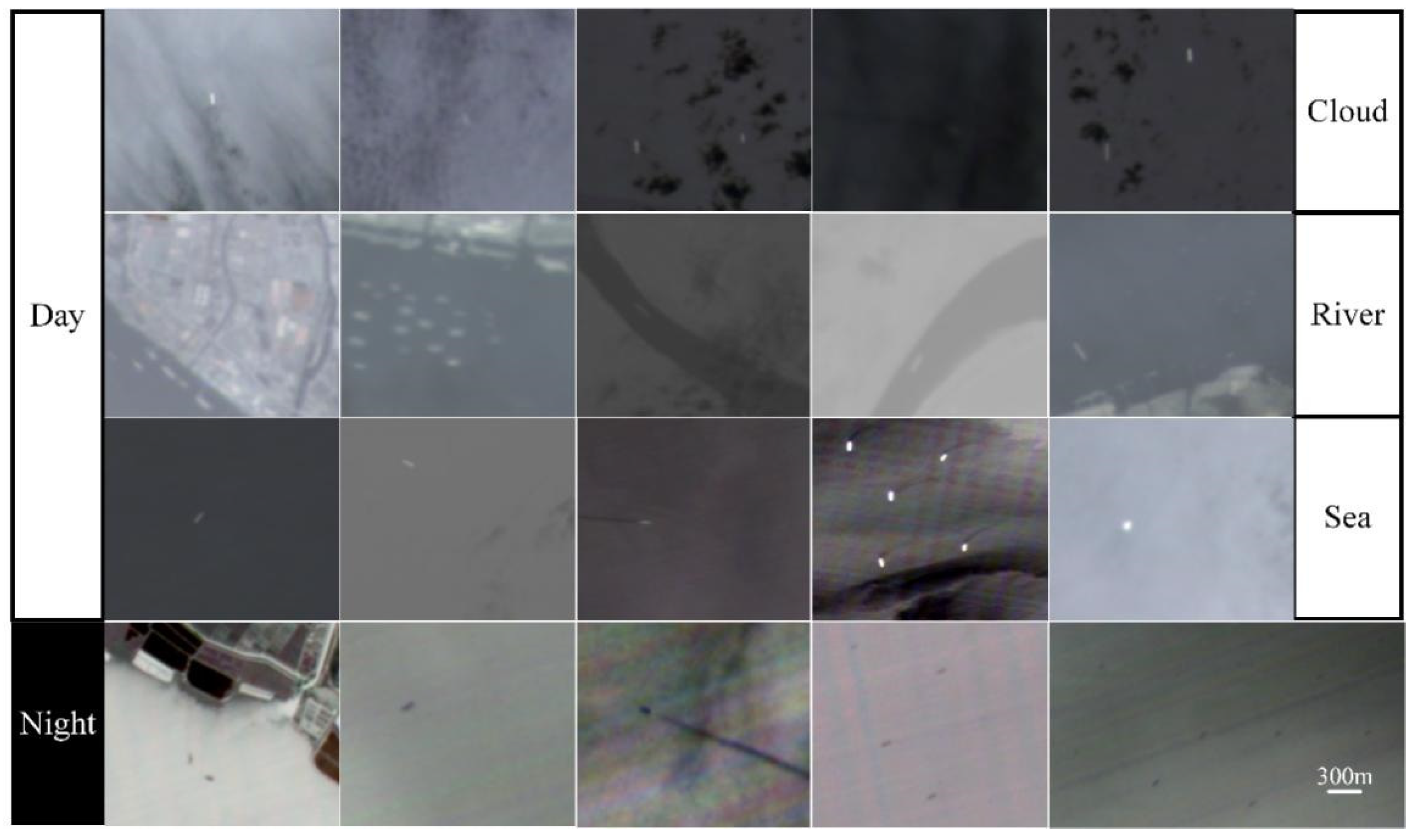
For the images with the same quantization level, there is a direct relationship between the standard deviation and the quantity of information. The standard deviation reflects the total dispersion between the gray value of each pixel and the mean of the image. To a certain extent, the larger the standard deviation, the greater the information content contained. The minimum, maximum, mean, and standard deviation of the three bands in our datasets are summarized in

Table 3. The statistics of digital numbers in the TISD’s images.

Basic Stats		Minimum	Maximum	Mean	Standard Deviation
Day	Band 1	0	255	95.4283	33.7011
	Band 2			102.6915	36.0583
	Band 3			94.7201	34.1300
night	Band 1			83.128962	32.2019
	Band 2			90.506944	33.0471
	Band 3			88.549713	32.2286

. The TISD contains day and night images of clouds, rivers, and sea scenes, as shown in Figure 6.

The correlation coefficient is related to the redundancy between different bands images. If it approaches or is 0, there is no correlation between bands. The correlation coefficient between B1: 11.5–12.5 µm and B3: 10.3–11.3 µm is larger than that of B1: 11.5–12.5 µm and B2: 8–10.5 µm, indicating that the images fused by B1 and B2 bands have less redundant information when they are input into the CNN, as shown in

Table 4. The summary of correlation coefficients.

Correlation		Band 1	Band 2	Band 3
Day	Band 1	1	-	-
	Band 2	0.9799	1	-
	Band 3	0.9921	0.9812	1
night	Band 1	1	-	-
	Band 2	0.9535	1	-
	Band 3	0.9672	0.9528	1

.

Combining standard deviation and correlation coefficient, Chavez proposed the optimum index factor ($OIF$) in 1982, as shown in Equation (9). Where $S_i$ is the standard deviation, $R_{ij}$ is the correlation coefficient of $i$ and $j$ channels, and n represents the combination of n bands. The larger the $OIF$, the greater the information content of the combined $n$ bands image. The band combination corresponding to a larger $OIF$ is the optimal scheme, as shown in

Table 5. The summary of dataset feature analysis.

Combination Bands		Cumulative Standard Deviation	Cumulative Correlation	Optimum Index Factor
Day	B12	69.7594	0.9799	35.5952
	B13	67.8311	0.9921	34.1856
	B23	70.1883	0.9812	35.7666
	B123	103.8894	2.9531	35.1792
Night	B12	65.2490	0.9535	34.2155
	B13	64.4305	0.9672	33.3077
	B23	65.2757	0.9528	34.2547
	B123	97.4776	2.8735	33.9230

.

$$OIF={\displaystyle \sum _{i=1}^n{S}_i/{\displaystyle \sum _{j=1}^n\left|R_{ij}\right|}}$$

(9)

4. Experimental Analysis

In this section, evaluation criteria, the proposed network (including experimental details and architecture of our method), comparative experiments (containing quantitative and qualitative results), and the fusion of glimmer and thermal infrared results are described in detail.

4.1. Evaluation Criteria

By using the proposed TISD dataset, the advanced algorithm is utilized for evaluation to establish relevance to the dataset feature analysis and a baseline for future research in the field. Precision is the correct positive class divided by all positive classes found, as shown in Equation (10). Recall is the correct positive class found divided by all the positive classes that should have been found, as in Equation (11). To be more comprehensive, the mean average accuracy (mAP) is the area enclosed by Precision and Recall as the two coordinate axes, as shown in Equation (12). Additionally, in [email protected], the number after @ is the threshold of intersection over union (IOU). The missing alarm (MA) is how many positive cases are missed, as shown in Equation (13). The false alarm (FA) is the number of negative cases misjudged to be positive cases, as shown in Equation (14).

$$\mathrm{Precision}=\frac{\mathrm{TP}}{\mathrm{TP}+\mathrm{FP}}$$

(10)

$$\mathrm{Recall}=\frac{\mathrm{TP}}{\mathrm{TP}+\mathrm{FN}}$$

(11)

$$\mathrm{mAP}=\underset{0}{\overset{1}{{\displaystyle \int }}}\mathrm{p}\left(\mathrm{r}\right)\mathrm{dr}$$

(12)

$$\mathrm{MA}=\frac{\mathrm{FN}}{\mathrm{TP}+\mathrm{FN}}=1-\mathrm{Recall}$$

(13)

$$\mathrm{FA}=\frac{\mathrm{FP}}{\mathrm{TP}+\mathrm{FP}}=1-\mathrm{Precision}$$

(14)

4.2. The Proposed Network

The one-stage algorithms omit the region proposal in the two-stage models and they directly predict spatially separated boundary boxes and related class probabilities. To achieve real-time actual ship detection in this paper, the advanced one-stage target detection frame is chosen. To verify the reliability of datasets and feature analysis, the improved YOLO-based algorithm is proposed to train and generate corresponding models by utilizing the TISD datasets of different bands. The architecture of proposed all-day ship detection methods is shown in Figure 7. Our experiments run on a personal computer with 64-bit Ubuntu 20.04.1 operating system. The software consists of Python, Torch 1.9.0, Conda 4.12.0, CUDA 11.3, and cuDNN 8.2.1.32. The hardware includes two NVIDIA GeForce RTX 3070s with 8 GB memory.

Our model is mainly divided into backbone, neck, and head. Based on our previous work [20], Dilated Conv is added in backbone to extract ships of different sizes. In the neck, SElayer is added to extract more important feature maps. Additionally, the details of these modules, including Focus, Ghost Bottleneck, and CSP1_X, are shown at the bottom in Figure 7. To achieve real-time ship detection on the satellite, we further lightweight the network by replacing ordinary convolution with depth-wise separable convolution in the head of the network. Compared with the state-of-the-art models, the number of floating-point operations (FLOPs) and parameters is greatly reduced in our model. GFLOPs is used to measure the complexity of an algorithm or model. The GFLOPs of our model is 8.2, which greatly reduces the amount of computation required by the models, of which Faster R-CNN [7] is 46.7, SSD [8] is 19.6, and Yolov5s [20] is 17.1. Additionally, our model has 390 layers, 3,244,653 parameters, and 3,244,653 gradients. The memory size of the saved model is 6.5 MB. The number of parameters of our model is 3.2 M, of which Faster R-CNN [7] is 31.3 M, SSD [8] is 138.0 M, and Yolov5s [20] is 7.3 M. The lower number of FLOPs required to process the same image on the same hardware allows for more images to be processed in the same amount of time. In general, the lower the number of network layers and parameters, the smaller the memory required to save the model, and the lower the hardware memory requirements. Therefore, compared with the mainstream methods, our model can be more easily deployed on the embedded platform.

4.3. Comparative Experiments

Using the same test set, the Precision, Recall, and [email protected] are compared. According to the datasets feature analysis in Section 3.3, the OIF of B12, B13, and B23 are 35.5952, 34.1856, and 35.7666, respectively. To a certain extent, the OIF is related to the available information, that is, the data of band B23 contains more information than that of B12 and B13.

After the learning the data, the Precision and Recall curve (PR curve) of the B23 model completely covers the PR curve of the B12 and B13 models; therefore, it can be asserted that the performance of B23 is better than that of B12 and B13. The PR curve of B12 and B13 intersect, so their performances can be compared based on the area under the curve. As shown in Figure 8, the model obtained by B23 is significantly better than that of B12 and B13, which is consistent with the analysis results of OIF.

In the lower left corner of Figure 9, a comprehensive evaluation index [email protected] in 200 epochs is selected for comparison. Moreover, the curves of 160~190 periods are amplified, and the mean average accuracy of combined band B23 is better than that of B12 and B13. In conclusion, there is a positive correlation between the band information content and the detection accuracy, and the trend of theoretical OIF analysis is consistent with that of [email protected]. The standard deviation of B1, B2, and B3 images with the same quantization level are 33.7011, 36.0583, and 34.1300, respectively. Theoretically, the information content of B2 is higher than that of B1 and B3. Empirically, the more channels information is input into the same CNN model, the higher the possibility of extracting richer features. As shown in Figure 9, compared with single band and combined band, the quantitative evaluation [email protected] of ship detection based on B23 datasets is the highest. In addition, the OIF of combined band B23 is also the highest, which means that increasing spectral channels is conducive to improving the target detection accuracy. Interestingly, [email protected] of B2 is slightly lower than that of B23, but almost equal to [email protected] of B12, which means that in the process of training CNN models, the input spectral channels should not be added blindly.

In the binary classification experiment, if the candidate sample is predicted to be a ship target, the classification result belongs to the ship; otherwise, it belongs to the non-ship. Single band and combined band data are used to train the optimal model for testing, and the evaluation criteria are shown in

Table 6. Detection evaluation criteria of single band and combined bands images in the TISD by several models (The bold data is the best result of the each model).

Methods	Bands	Image Size	Precision	Recall	[email protected]	Val_loss
Faster R-CNN [7]	B1	768 × 768	0.5907	0.3628	0.3367	0.0277
	B2		0.6986	0.6739	0.6682	0.0168
	B3		0.7193	0.6263	0.6504	0.0195
	B12		0.6729	0.6326	0.5917	0.0191
	B23		0.7473	0.7116	0.6758	0.0190
	B13		0.6683	0.5907	0.5897	0.0231
SSD [8]	B1	768 × 768	0.6711	0.4977	0.5179	0.02322
	B2		0.7492	0.6000	0.6544	0.01399
	B3		0.7222	0.6651	0.6304	0.01958
	B12		0.7159	0.6681	0.6676	0.01838
	B23		0.7208	0.6977	0.7102	0.01771
	B13		0.6853	0.6186	0.6049	0.02128
The improved Yolov5s	B1	640 × 640	0.6818	0.4791	0.4719	0.0236
	B2		0.7212	0.7349	0.7031	0.0178
	B3		0.6619	0.6356	0.6189	0.0191
	B12		0.7003	0.6419	0.6047	0.0190
	B23		0.7929	0.7300	0.7395	0.0150
	B13		0.6244	0.6279	0.5771	0.0214

. The Precision and Recall of B23, B2, and B123 ranked the top three. By analyzing the dataset features of standard deviation, correlation coefficients, and OIF, best spectrum channels combination can be selected during training, which is conducive to the improvement of target detection accuracy.

Through the evaluation in the TISD, the detection accuracy in the cloudy images is lower than that in the cloud-free images, therefore, broken clouds are the main false alarms during ship detection, as shown in

Table 7. The evaluation criteria of different methods by using the TISD (The bold data are the best and second-best results of different models).

Methods	Bands	Scene	Image Size	Precision	Recall	[email protected]	Val_loss	GFLOPs	Parameters
Faster R-CNN [7]	B123	ALL	768 × 768	0.6617	0.6372	0.5998	0.0221	46.7	31.3 M
SSD [8]	B123	ALL	768 × 768	0.6915	0.6791	0.6572	0.0189	19.6	138.0 M
Yolov5s [20]	B123	ALL	640 × 640	0.7668	0.6308	0.6618	0.0096	17.1	7.3 M
The improved Yolov5s	B123	ALL	640 × 640	0.7485	0.6651	0.6378	0.0187	8.2	3.2 M
		Cloud		0.6925	0.4948	0.4983	0.0114
		River		0.7637	0.5173	0.5444	0.0194
		Sea		0.8150	0.7132	0.7163	0.0044
		Day		0.7864	0.6424	0.6768	0.0097
		Night		0.6165	0.4143	0.4246	0.0119

. In cloud, river and sea scenes, the detection accuracy on the sea surface is the highest, up to 81.15%.

Based on the proposed datasets, a round-the-clock ship detection model can be obtained. The prediction results during day and night are shown in Figure 10 and Figure 11, and the quantitative evaluation summary is shown in

Table 8. Ship detection results for different scenarios and times.

Area	Time	False Alarm	Missing Alarm
Figure 10a. Shanghai Port	about 21 o’clock at night	5.71%	5.71%
Figure 10b. Sea near Pudong Airport		11.11%	11.11%
Figure 11a. Tianjin Port	about 10 o’clock in the day	0.68%	3.29%
Figure 11b. Partial Sea of Bohai		1.64%	7.69%

.

4.4. Fusion of Glimmer and Thermal Infrared

Glimmer sensor is an active application in the field of remote sensing, which can obtain visible light emitted from the surface without cloudlessness at night. Most of the information at night is related to human activities, such as city lights and ship lights. Compared with daytime images, the information at night can be directly captured by glimmer sensors to depict human fine activities. According to the differences of imaging technologies, the detection results of glimmer sensors can increase the reliability of thermal infrared detection results. As shown in Figure 12a, the positive ship detection results of thermal infrared image are marked in yellow boxes, totaling 91. The ships observed by glimmer data are marked in blue boxes in Figure 12b, totaling 42. In Figure 12c, the yellow boxes are the ships observed in the thermal infrared image but not in the glimmer data, and blue boxes are the ships observed by both.

5. Discussion

As an important military target, real-time ship detection throughout the day has great military significance. Many scholars have studied the effectiveness and generalization of models using public datasets. However, due to the lack of infrared images, there are few available thermal infrared ship datasets. In this paper, a thermal infrared three-channel ship dataset is proposed, and a complete ship detection network model is designed based on the regression algorithm. Unlike visible remote sensing data, our dataset contains ships at night. As opposed to the simulation data, the dataset we propose uses real remote sensing images, which is more conducive to real-time target detection on the satellite. The TISD is based on three-channel thermal infrared images of the SDGSAT-1 thermal imaging system, and the Landsat-8 thermal infrared sensor only has two channels. The TISD has an additional band, namely 8~10.5 µm; therefore, the proposed dataset contains rich spectral information. Dataset feature analysis in Section 3.4 and the experimental results in Table 6 show that the increase of spectral information is more conducive to target detection. Instead of utilizing two-stage algorithms, our model is based on a one-stage Yolov5s, which is more conductive to speeding up prediction. In our model, dilated convolution can extract more fine features for smaller ships, and SElayer can pick out more important features. As shown in Table 7, the accuracy of the proposed model is higher than that of other advanced models in sea scenes. In complex scenes, with a slight decrease of accuracy, our model parameters and floating-point operations are greatly reduced, where our model’s FLOPs is only 47.95% of original Yolov5s’ FLOPs. Thus, it is possible to detect ships from thermal infrared remote sensing images based on the lightweight Yolov5s model.

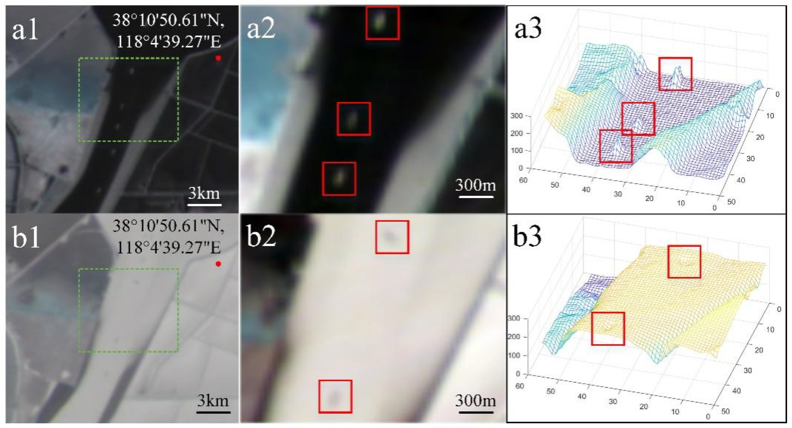
However, the following aspects can be further studied. First, there is an object on land that is misidentified as a ship, as shown by the yellow box in Figure 11a. Due to the complex situation of land surface, target detection in the sea can be carried out after the preprocessing of sea and land segmentation in the future work. Second, in Table 7, the accuracy detection at nighttime is lower than during the daytime. The possible reason is that the temperature difference between the ship and the water is too small at night, resulting in a weak contrast between the intensity of target and the background. In Figure 13a3, during the day, the intensity of the boat is much higher than that of the water. As shown in Figure 13b3, at night, the intensity of the ship is slightly lower than that of the water, resulting in a low signal-to-background ratio, which is not conducive to target detection. Later work should be scheduled to increase the nighttime ship dataset and to augment the target signal. Third, due to different imaging technology, glimmer datasets are a good complement for thermal infrared images. Our future work will focus on the expansion of glimmer datasets and ship wake labeling to promote accurate ship detection at night.

6. Conclusions

In this paper, the difficulties of existing ship detection datasets are summarized. Due to the high secrecy level of infrared data, thermal infrared ship datasets are lacking. Moreover, both detection accuracy and speed need to be considered for ship detection.

Aiming at the above problems, to the best of our knowledge, we are the first to annotate the three-bands thermal infrared ship dataset (TISD) to compensate for the lack of spaceborne thermal infrared public datasets. All images are provided from the SDGSAT-1 satellite thermal imaging system and all ship targets are annotated with high-precision boundary boxes. After band-to-band registration and up-sampling, the TISD currently contains 2190 images with a resolution of 10 m and 12,774 targets with a wide aspect ratio. The dataset is carefully selected to cover river and sea scenes at different imaging times and with different amounts of cloud cover.

By utilizing TISD, an all-day ship detection model is trained by an improved YOLO-based detector. Experiments show that the result of proposed method is excellent, and especially the detection accuracy on the sea surface is the highest, up to 81.15%. In cloudy, and river scenes, with a slight decrease of accuracy, the computational complexity of the proposed algorithm is greatly reduced, where our model’s FLOPs is only 47.95% of original Yolov5s’ FLOPs.

Based on data feature analyses, the optimal bands combination can promote the accuracy of detection. Among them, the standard deviation is proportional to the information, and the correlation coefficient between bands is related to redundancy data of different bands. Optimum index factor is used to combine standard deviation and correlation coefficient. By experimental comparisons of different bands, optimum index factor is positively correlated with the detection accuracy to a certain extent.

Combined with glimmer images, the model based on TISD is verified to be capable of all-day ship detection. In practice, the proposed dataset is expected to promote the research and application of all-day spaceborne ship detection.

References

1. Zhao, D.; Zhu, C.; Qi, J.; Qi, X.; Su, Z.; Shi, Z. Synergistic Attention for Ship Instance Segmentation in SAR Images. Remote Sens. 2021, 13, 4384. [Google Scholar] [CrossRef]
2. Kang, K.M.; Kim, D.J. Ship Velocity Estimation From Ship Wakes Detected Using Convolutional Neural Networks. IEEE J. Sel. Top. Appl. Earth Obs. Remote Sens. 2019, 12, 4379–4388. [Google Scholar] [CrossRef]
3. Yang, G.; Li, B.; Ji, S.; Gao, F.; Xu, Q. Ship Detection from Optical Satellite Images Based on Sea Surface Analysis. IEEE Geosci. Remote Sens. Lett. 2014, 11, 641–645. [Google Scholar] [CrossRef]
4. Zhu, C.; Zhou, H.; Wang, R.; Guo, J. A Novel Hierarchical Method of Ship Detection from Spaceborne Optical Image Based on Shape and Texture Features. IEEE Trans. Geosci. Remote Sens. 2010, 48, 3446–3456. [Google Scholar] [CrossRef]
5. Girshick, R.; Donahue, J.; Darrell, T.; Malik, J. Rich feature hierarchies for accurate object detection and semantic segmentation. In Proceedings of the Computer Vision and Pattern Recognition (CVPR), Columbus, OH, USA, 23–28 June 2014. [Google Scholar]
6. Girshick, R. Fast R-CNN. In Proceedings of the IEEE International Conference on Computer Vision (ICCV), Santiago, Chile, 7–13 December 2015; pp. 1440–1448. [Google Scholar] [CrossRef]
7. He, S.; Girshick, K.; Sun, R.J. Faster R-CNN: Towards Real-Time Object Detection with Region Proposal Networks. IEEE Trans. Pattern Anal. Mach. Intell. 2017, 39, 1137–1149. [Google Scholar]
8. Liu, W.; Anguelov, D.; Erhan, D.; Szegedy, C.; Reed, S.; Fu, C.Y.; Berg, A.C. SSD: Single shot MultiBox detector. In Proceedings of the European Conference on Computer Vision (ECCV), Amsterdam, The Netherlands, 8–16 October 2016; pp. 21–37. [Google Scholar]
9. Liu, S.; Huang, D.; Wang, Y. Receptive field block net for accurate and fast object detection. In Proceedings of the European Conference on Computer Vision (ECCV), Munich, Germany, 8–14 September 2018; pp. 385–400. [Google Scholar]
10. Redmon, J.; Divvala, S.; Girshick, R.; Farhadi, A. You only look once: Unified real-time object detection. In Proceedings of the IEEE Conference on Computer Vision and Pattern Recognition (CVPR), Las Vegas, NV, USA, 27–30 June 2016; pp. 779–788. [Google Scholar]
11. Redmon, J.; Farhadi, A. YOLO9000: Better faster stronger. In Proceedings of the IEEE Conference on Computer Vision and Pattern Recognition (CVPR), Honolulu, HI, USA, 21–26 July 2017; pp. 6517–6525. [Google Scholar]
12. Redmon, J.; Farhadi, A. YOLOv3: An incremental improvement. In Proceedings of the IEEE Conference on Computer Vision and Pattern Recognition (CVPR), Salt Lake City, UT, USA, 8 April 2018; Available online: https://arxiv.org/abs/1804.02767 (accessed on 8 April 2018).
13. Deng, J.; Dong, W.; Socher, R.; Li, L.J.; Li, K.; Li, F. ImageNet: A large-scale hierarchical image database. In Proceedings of the 2009 IEEE Conference on Computer Vision and Pattern Recognition (CVPR), Kyoto, Japan, 10 March 2009; pp. 248–255. [Google Scholar]
14. Everingham, M.; Van Gool, L.; Williams, C.K.I.; Winn, J.; Zisserman, A. The PASCAL Visual Object Classes (VOC) Challenge. Int. J. Comput. Vis. 2010, 88, 303–338. [Google Scholar] [CrossRef] [Green Version]
15. Lin, T.Y.; Maire, M.; Belongie, S.; Hays, J.; Perona, P.; Ramanan, D.; Dollár, P.; Zitnick, C.L. Microsoft COCO: Common objects in context. In Proceedings of the 13th European Conference on Computer Vision (ECCV), Zurich, Switzerlan, 6–12 September 2014; pp. 740–755. [Google Scholar]
16. Xia, G.S.; Bai, X.; Ding, J.; Zhu, Z.; Belongie, S.; Luo, J.; Datcu, M.; Pelillo, M.; Zhang, L. DOTA: A Large-Scale Dataset for Object Detection in Aerial Images. In Proceedings of the 2018 IEEE/CVF Conference on Computer Vision and Pattern Recognition (CVPR), Salt Lake City, UT, USA, 18–23 June 2018; pp. 3974–3983. [Google Scholar] [CrossRef] [Green Version]
17. Sun, X.; Wang, P.J.; Yan, Z.Y.; Xu, F.; Wang, R.; Diao, W.; Chen, J.; Li, J.; Feng, Y.; Xu, T.; et al. FAIR1M: A benchmark dataset for fine-grained object recognition in high-resolution remote sensing imagery. ISPRS J. Photogramm. Remote Sens. 2022, 184, 116–130. [Google Scholar] [CrossRef]
18. Qi, X.; Zhu, P.; Wang, Y.; Zhang, L.; Peng, J.; Wu, M.; Chen, J.; Zhao, X.; Zang, N.; Mathiopoulos, P.T. MLRSNet: A multi-label high spatial resolution remote sensing dataset for semantic scene understanding. ISPRS J. Photogramm. Remote Sens. 2020, 169, 337–350. [Google Scholar] [CrossRef]
19. Zhou, W.X.; Newsam, S.; Li, C.; Shao, Z. PatternNet: A benchmark dataset for performance evaluation of remote sensing image retrieval. ISPRS J. Photogramm. Remote Sens. 2018, 145, 197–209. [Google Scholar] [CrossRef]
20. Li, L.; Jiang, L.; Zhang, J.; Wang, S.; Chen, F. A Complete YOLO-Based Ship Detection Method for Thermal Infrared Remote Sensing Images under Complex Backgrounds. Remote Sens. 2022, 14, 1534. [Google Scholar] [CrossRef]
21. Gao, Y.; Gao, F.; Dong, J.; Wang, S. Change Detection from Synthetic Aperture Radar Images Based on Channel Weighting-Based Deep Cascade Network. IEEE J. Sel. Top. Appl. Earth Obs. Remote Sens. 2019, 12, 4517–4529. [Google Scholar] [CrossRef]
22. Giustarini, L.; Hostache, R.; Matgen, P.; Schumann, G.J.; Bates, P.D.; Mason, D.C. A Change Detection Approach to Flood Mapping in Urban Areas Using TerraSAR-X. IEEE Trans. Geosci. Remote Sens. 2013, 51, 2417–2430. [Google Scholar] [CrossRef] [Green Version]
23. Zhao, Y.; Zhao, L.; Xiong, B.; Kuang, G. Attention Receptive Pyramid Network for Ship Detection in SAR Images. IEEE J. Sel. Top. Appl. Earth Obs. Remote Sens. 2020, 13, 2738–2756. [Google Scholar] [CrossRef]
24. Wang, X.; Chen, C. Ship Detection for Complex Background SAR Images Based on a Multiscale Variance Weighted Image Entropy Method. IEEE Geosci. Remote Sens. Lett. 2017, 14, 184–187. [Google Scholar] [CrossRef]
25. Ai, J.; Qi, X.; Yu, W.; Deng, Y.; Liu, F.; Shi, L. A New CFAR Ship Detection Algorithm Based on 2-D Joint Log-Normal Distribution in SAR Images. IEEE Geosci. Remote Sens. Lett. 2010, 7, 806–810. [Google Scholar] [CrossRef]
26. Gong, M.; Cao, Y.; Wu, Q. A Neighborhood-Based Ratio Approach for Change Detection in SAR Images. IEEE Geosci. Remote Sens. Lett. 2012, 9, 307–311. [Google Scholar] [CrossRef]
27. Zhang, Y.; Wang, S.; Wang, C.; Li, J.; Zhang, H. SAR Image Change Detection Using Saliency Extraction and Shearlet Transform. IEEE J. Sel. Top. Appl. Earth Obs. Remote Sens. 2018, 11, 4701–4710. [Google Scholar] [CrossRef]
28. Song, J.; Kim, D.J.; Kang, K.M. Automated procurement of training data for machine learning algorithm on ship detection using AIS information. Remote Sens. 2020, 12, 1443. [Google Scholar] [CrossRef]
29. Rostami, M.; Kolouri, S.; Eaton, E.; Kim, K. Deep transfer learning for few-shot SAR image classification. Remote Sens. 2019, 11, 1374. [Google Scholar] [CrossRef]
30. Huang, L.; Liu, B.; Li, B.; Guo, W.; Yu, W.; Zhang, Z.; Yu, W. OpenSARShip: A Dataset Dedicated to Sentinel-1 Ship Interpretation. IEEE J. Sel. Top. Appl. Earth Obs. Remote Sens. 2018, 11, 195–208. [Google Scholar] [CrossRef]
31. Zhang, T.; Zhang, X.; Li, J.; Xu, X.; Wang, B.; Zhan, X.; Xu, Y.; Ke, X.; Zeng, T.; Su, H.; et al. SAR Ship Detection Dataset (SSDD): Official Release and Comprehensive Data Analysis. Remote Sens. 2021, 13, 3690. [Google Scholar] [CrossRef]
32. Sun, X.; Wang, Z.R.; Sun, Y.R.; Diao, W.; Zhang, Y.; Fu, K. AIR-SARShip-1.0: High-resolution SAR ship detection dataset. J. Radars 2019, 8, 852–862. [Google Scholar] [CrossRef]
33. Wang, Y.; Wang, C.; Zhang, H.; Dong, Y.; Wei, S. A SAR Dataset of Ship Detection for Deep Learning under Complex Backgrounds. Remote Sens. 2019, 11, 765. [Google Scholar] [CrossRef] [Green Version]
34. Wei, S.; Zeng, X.; Qu, Q.; Wang, M.; Su, H.; Shi, J. HRSID: A High-Resolution SAR Images Dataset for Ship Detection and Instance Segmentation. IEEE Access 2020, 8, 120234–120254. [Google Scholar] [CrossRef]
35. Law, H.; Deng, J. CornerNet: Detecting objects as paired keypoints. In Proceedings of the European Conference on Computer Vision (ECCV), Munich, Germany, 8–14 September 2018; pp. 734–750. [Google Scholar]
36. Cui, Z.; Leng, J.; Liu, Y.; Zhang, T.; Quan, P.; Zhao, W. SKNet: Detecting Rotated Ships as Keypoints in Optical Remote Sensing Images. IEEE Trans. Geosci. Remote Sens. 2021, 59, 8826–8840. [Google Scholar] [CrossRef]
37. Han, Y.; Yang, X.; Pu, T.; Peng, Z. Fine-Grained Recognition for Oriented Ship Against Complex Scenes in Optical Remote Sensing Images. IEEE Trans. Geosci. Remote Sens. 2022, 60, 1–18. [Google Scholar] [CrossRef]
38. Shao, Z.; Wu, W.; Wang, Z.; Du, W.; Li, C. SeaShips: A Large-Scale Precisely Annotated Dataset for Ship Detection. IEEE Trans. Multimed. 2018, 20, 2593–2604. [Google Scholar] [CrossRef]
39. Wang, Z.; Zhou, Y.; Wang, F.; Wang, S.; Xu, Z. SDGH-Net: Ship detection in optical remote sensing images based on Gaussian heatmap regression. Remote Sens. 2021, 13, 499. [Google Scholar] [CrossRef]
40. Li, Z.; You, Y.; Liu, F. Analysis on Saliency Estimation Methods in High-Resolution Optical Remote Sensing Imagery for Multi-Scale Ship Detection. IEEE Access 2020, 8, 194485–194496. [Google Scholar] [CrossRef]
41. Yao, Y.; Jiang, Z.; Zhang, H.; Zhao, D.; Cai, B. Ship detection in optical remote sensing images based on deep convolutional neural networks. J. Appl. Remote Sens. 2017, 11, 042611. [Google Scholar] [CrossRef]
42. Zhang, S.; Wu, R.; Xu, K.; Wang, J.; Sun, W. R-CNN-based ship detection from high resolution remote sensing imagery. Remote Sens. 2019, 11, 631. [Google Scholar] [CrossRef] [Green Version]
43. Li, H.; Deng, L.; Yang, C.; Liu, J.; Gu, Z. Enhanced YOLO v3 Tiny Network for Real-Time Ship Detection from Visual Image. IEEE Access 2021, 9, 16692–16706. [Google Scholar] [CrossRef]
44. Shao, Z.; Wang, L.; Wang, Z.; Du, W.; Wu, W. Saliency-Aware Convolution Neural Network for Ship Detection in Surveillance Video. IEEE Trans. Circuits Syst. Video Technol. 2020, 30, 781–794. [Google Scholar] [CrossRef]
45. Wang, N.; Li, B.; Wei, X.; Wang, Y.; Yan, H. Ship Detection in Spaceborne Infrared Image Based on Lightweight CNN and Multisource Feature Cascade Decision. IEEE Trans. Geosci. Remote Sens. 2021, 59, 4324–4339. [Google Scholar] [CrossRef]
46. Song, Z.; Yang, J.; Zhang, D.; Wang, S.; Li, Z. Semi-Supervised Dim and Small Infrared Ship Detection Network Based on Haar Wavelet. IEEE Access 2021, 9, 29686–29695. [Google Scholar] [CrossRef]
47. Li, Y.; Li, Z.; Ding, Z.; Qin, T.; Xiong, W. Automatic Infrared Ship Target Segmentation Based on Structure Tensor and Maximum Histogram Entropy. IEEE Access 2020, 8, 44798–44820. [Google Scholar] [CrossRef]
48. Bloisi, D.D.; Iocchi, L.; Pennisi, A.; Tombolini, L. ARGOS-venice boat classification. In Proceedings of the 12th IEEE Conference on Advanced Video and Signal Based Surveillance (AVSS), Karlsruhe, Germany, 25–28 August 2015; pp. 1–6. [Google Scholar]
49. Patino, L.; Cane, T.; Vallee, A.; Ferryman, J. PETS 2016: Dataset and challenge. In Proceedings of the IEEE Conference on Computer Vision and Pattern Recognition Workshops (CVPRW), Las Vegas, NV, USA, 26 June–1 July 2016; pp. 1240–1247. [Google Scholar]
50. Cui, H.; Li, L.; Liu, X.; Su, X.; Chen, F. Infrared Small Target Detection Based on Weighted Three-Layer Window Local Contrast. IEEE Geosci. Remote Sens. Lett. 2022, 19, 1–5. [Google Scholar] [CrossRef]
51. Chen, Y.; Li, L.; Liu, X.; Su, X. A Multi-Task Framework for Infrared Small Target Detection and Segmentation. IEEE Trans. Geosci. Remote Sens. 2022, 60, 1–9. [Google Scholar] [CrossRef]
52. Kang, M.; Kim, K. Automatic SAR Image Registration via Tsallis Entropy and Iterative Search Process. IEEE Sens. J. 2020, 20, 7711–7720. [Google Scholar] [CrossRef]
Figure 1. (a) The SAR image with the resolution of 15 m in SSDD dataset [31], The (b) true color image of 460–520 nm, 520–600 nm and 630–690 nm with resolution of 10 m in 38°44′32.74″N,117°50′13.28″E from SDGSAT-1 multispectral imager, and (c) pseudo-color image of 8~10.5 µm, 10.3~11.3 µm, 11.5~12.5 µm with resolution of 30 m in 39°18′49.52″N,120°14′55.86″E from SDGSAT-1 TIS.
Remotesensing 14 05297 g001
Figure 2. The intensity images of B1: 11.5~12.5 µm, B2: 8~10.5 µm, B3: 10.3~11.3 µm. The brightness temperature on the pupil (T/K) are marked in the color bar, and the three-bands pseudo-color image with the resolution of 30 m in Yellow Sea of China from SDGSAT-1 TIS is shown in the bottom left. The digital number (DN) of the ship and sea surface and the brightness temperature on the pupil (T/K) of the ship and sea surface are shown in the table on the right. The horizontal pixels offset of B1–B2 and B2–B3 is thirty pixels, and the vertical pixels offset of B1–B2 and B2–B3 is two pixels, as shown on the bottom right.
Remotesensing 14 05297 g002
Figure 3. PASCAL VOC XML annotation for 768 × 768 three-bands pseudo-color images with the resolution of 10 m. (351,243) and (388,283) are, respectively, the coordinates of the top left and bottom right of the bounding boxes of the left ships.
Remotesensing 14 05297 g003
Figure 4. Statistical results of ship target bounding box length and width in the TISD dataset.
Remotesensing 14 05297 g004
Figure 5. Statistical results of (a) aspect ratio of ship target bounding box and (b) the brightness temperature on the pupil (T/K) between the ships and sea surface in 8~10.5 µm in the TISD.
Remotesensing 14 05297 g005aRemotesensing 14 05297 g005b
Figure 6. Parts of day and night images in the cloud, river, and sea scenes of the TISD.
Remotesensing 14 05297 g006
Figure 7. The architecture of proposed all-day ship detection methods (The details of these modules including Focus, Ghost Bottleneck, and CSP1_X are shown at the bottom).
Remotesensing 14 05297 g007
Figure 8. The Precision and Recall curve of combined bands B23, B12, and B13.
Remotesensing 14 05297 g008
Figure 9. The [email protected] of combined bands B23, B12, B13, and single band B1, B2, B3 in 200 epochs.
Remotesensing 14 05297 g009
Figure 10. The results of nighttime ship detection by using the TISD in (a) Shanghai Port and (b) sea near Pudong Airport. (The red boxes show the correct vessel detected, the yellow boxes show false alarms, and the blue boxes show missing alarms).
Remotesensing 14 05297 g010
Figure 11. The results of daytime ship detection by using the TISD in (a) Tianjin Port and (b) Partial Sea of Bohai during daytime. (The red boxes show the correct vessel detected, the yellow box shows the false alarm, and the blue boxes show the missing alarms).
Remotesensing 14 05297 g011
Figure 12. Night images in Mumbai, India with (a) thermal infrared image of 11.5–12.5 µm, 8–10.5 µm, and 10.3–11.3 µm at night (The positive ship detection results are marked in yellow boxes), (b) glimmer image of R:615~690 nm, G:520~615 nm, and B:430~520 nm at night (The observed ships are marked in blue boxes), (c) fusion image of 0.615~0.69 nm, 8~10.5 µm, and 10.3~11.3 µm with the resolution of 10 m (Ships observed in the thermal infrared image but not in the glimmer data are marked in yellow boxes, and ships observed by both are marked in blue boxes), (d) an enlarged image of the green box in c.
Remotesensing 14 05297 g012
Figure 13. (a1) the daytime image at Bohai port in 38°10′50.61″N,118°4′39.27″E (a2) an enlarged image of the green box in a1, (a3) the intensity distribution of a2, (b1) the images at night in the same area as a1, (b2) an enlarged image of the green box in b1, and (b3) intensity distribution of b2 (The red boxes are the ships).
Remotesensing 14 05297 g013