Abstract
The occlusion of cloud layers affects the accurate acquisition of ground object information and causes a large amount of useless remote-sensing data transmission and processing, wasting storage, as well as computing resources. Therefore, in this paper, we designed a lightweight composite neural network model to calculate the cloud amount in high-resolution visible remote-sensing images by training the model using thumbnail images and browsing images in remote-sensing images. The training samples were established using paired thumbnail images and browsing images, and the cloud-amount calculation model was obtained by training a proposed composite neural network. The strategy used the thumbnail images for preliminary judgment and the browsing images for accurate calculation, and this combination can quickly determine the cloud amount. The multi-scale confidence fusion module and bag-of-words loss function were redesigned to achieve fast and accurate calculation of cloud-amount data from remote-sensing images. This effectively alleviates the problem of low cloud-amount calculation, thin clouds not being counted as clouds, and that of ice and clouds being confused as in existing methods. Furthermore, a complete dataset of cloud-amount calculation for remote-sensing images, CTI_RSCloud, was constructed for training and testing. The experimental results show that, with less than 13 MB of parameters, the proposed lightweight network model greatly improves the timeliness of cloud-amount calculation, with a runtime is in the millisecond range. In addition, the calculation accuracy is better than the classic lightweight networks and backbone networks of the best cloud-detection models.
1. Introduction
With the development of space technology and the continuous launch of remote-sensing satellites, the data volume of remote-sensing images has seen rapid growth. Statistics show that, continuously, more than 66% of the Earth’s surface is covered by clouds [1], which makes the ground observation of optical remote-sensing images challenging. Additionally, this causes many optical remote-sensing images to become cloudy and thus be judged as invalid data. The general processing method implements cloud-detection methods to exclude the interference of cloud regions, remove redundant and invalid data to some extent, and concentrate the subsequent image interpretation on the cloud-free images or regions. However, two scenarios require new consideration: the processing of in-orbit remote sensing and the management of enormous remote-sensing images. Since the computing and storage capabilities of the in-orbit platform are constrained, a simple and efficient cloud-amount calculation method is urgently required. To manage nearly ten million different types of remote-sensing images, the management system for huge remote-sensing images generally adopts a database server and a disk array. At the same time, the system itself has limited computing power. When the cloud judgment of remote-sensing data before warehousing is not accurate enough, it introduces difficulties to subsequent user retrieval and data usage. Therefore, a method that is less computationally intensive and can calculate the cloud amount of remote-sensing images more accurately without directly calculating the original images is needed to ensure the efficient operation of data management.
With the development of remote-sensing image processing, cloud detection and amount calculation has been an important research topic. Numerous representative methods [2,3,4,5,6,7,8,9] have been proposed to solve this challenge. These methods fall into two main categories: threshold-based methods and statistical-based methods. The former sets a threshold to detect clouds based on information such as spectral reflectance, brightness, and temperature. However, this threshold is not global and does not apply to all scenarios. Therefore, its value must be set according to the different remote-sensing images to be processed. The statistical-based approach is to design manual features based on the physical properties of the cloud (e.g., texture, geometric relationships, and color) and then to use statistical machine-learning methods to classify them pixel by pixel. This method also calculates the cloud amount of the whole image, which facilitates the qualitative and quantitative analysis of remote-sensing images by operators. However, such statistical machine learning-based methods are completely dependent on the feature design level of the researchers. These methods do not work well in practical applications, mainly because the environment captured by remote-sensing images is so diverse that it is difficult to meet the requirements of stability applications.
The rapid development of deep learning in recent years has led to the application of methods involving deep convolutional neural networks to cloud detection, which has facilitated the rapid development of cloud detection and cloud-amount computing due to its very powerful feature representation and scene application capabilities [10,11,12,13,14,15,16,17,18]. The convolutional neural network-based approach can achieve automatic feature acquisition and automatic classification by establishing a nonlinear mapping from input to output. Experiments have proved that with enough representative samples, better cloud detection and cloud-amount calculation results can be obtained through continuous training and learning. The convolutional neural network-based approach has achieved the best results to date, but it still faces some problems and limitations.
First, most existing CNN-based models improve the performance of cloud detection and cloud-amount calculation by increasing the width and depth of neural networks. Therefore, to obtain a higher accuracy of cloud detection, greater computational resources are required. Such huge neural network models limit their ability to be applied in resource-constrained situations, such as in-orbit processing and data management centers. It is also important to note that the variability in the shape and size of the clouds themselves, as well as the complexity of the background, makes cloud detection and cloud-amount calculation extremely challenging.
As shown in Figure 1 featuring thumbnails of original remote-sensing images, there are many disruptive factors and difficult situations in cloud detection and cloud-amount calculation. The eight remote-sensing images in Figure 1 are derived from ChineseGF-series satellites and ZY-series satellites. In Figure 1a, there is a certain degree of integration between clouds and ground objects. At the same time, a semi-transparent situation also exists. In the original cloud-amount calculation software, the cloud amount is only 12 (a percentage of the whole image), but as can be seen by visual interpretation, it is much more than 12. Thin clouds in Figure 1b are not calculated into the cloud amount by the general algorithm, which is obviously not accurate enough. The clouds in Figure 1c obscure almost all the ground objects, which is an invalid image. Additionally, the original cloud-calculation software calculates it as 8, which is not accurate enough either. In cloud-amount calculation, ice and thin clouds existing in Figure 1d are easily confused, which affects the accuracy of the calculation. The situation in Figure 1e is more complicated: there are thick clouds, thin clouds, ice, and snow, and the thin clouds are not distinguished from the ground objects. There are mainly thin clouds in Figure 1f, and they are evenly distributed throughout the whole image, making it difficult to calculate the cloud amount. In Figure 1g, there is mainly snow and ice and no clouds, but the original cloud-calculation software calculates them as clouds. In Figure 1h, there is a thick cloud almost completely covering the whole map, and the original cloud-calculation software calculates it as 0, which is clearly wrong. In summary, thin clouds, snow and ice interference, background and cloud integration, and other issues greatly complicate cloud-amount calculation.
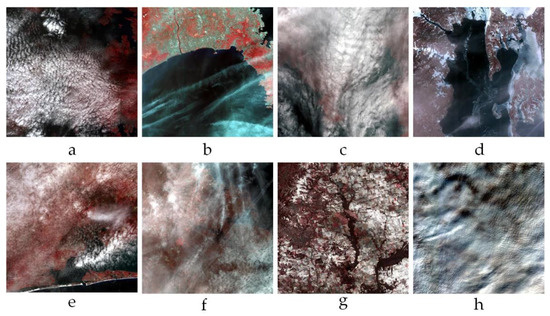
Figure 1.
Analysis diagram of some challenging examples of cloud detection in remote-sensing images, featuring: (a) a certain degree of integration between clouds and ground objects; (b) thin cloud not calculated as part of the cloud amount; (c) cloud obscuring almost all the ground objects; (d) ice and thin clouds that can be easily confused; (e) thick clouds, thin clouds, ice, and snow; (f) thin clouds evenly distributed throughout the whole image; (g) mainly snow and ice; (h) thick cloud almost completely covering the whole image.
Therefore, it is highly significant in research and application to design an efficient and lightweight neural network model to solve the above-mentioned difficulties. Among them, the most straightforward approach is to design the model with as few parameters and operators as possible. Based on what has been mentioned above, a ShuffleCloudNet network structure for cloud-amount computation is designed in this paper. In contrast to the traditional neural network model, ShuffleCloudNet is inspired by the unique operation structure of the channel split in ShuffleNetV2. Furthermore, it adopts the concatenation operation to obtain the perception ability of small-sized clouds. Moreover, the physical features of clouds are very complex and variable. To overcome this challenge, this paper designs a relevant multi-scale confidence fusion module to enhance the distinguishability of different backgrounds and foregrounds. Furthermore, this paper also defines a bag-of-words loss function so that the model can be optimized during the training process and thereby more directly distinguish cloud boundaries, small clouds, etc., from complex backgrounds (e.g., desert, seawater, glaciers, and snow). From the engineering practice experience of remote-sensing image management, we found that thumbnail images and browsing images in remote-sensing images contain good cloud cover information. Operators in the remote-sensing field often pay attention to the general cloud amount in the remote-sensing image rather than the specific cloud location. Therefore, we divide the cloud amount into 11 levels, 0–10, which simplifies the cloud-amount calculation.
To summarize, the main contributions of this paper can be outlined as follows.
- Differing from the traditional CNN method, an efficient and lightweight network model architecture for remote-sensing image cloud-amount computation is constructed, referred to as ShuffleCloudNet, and which can use fewer model parameters to obtain better results of cloud-amount computation.
- Based on the diversity of clouds and the complexity of backgrounds, a multi-scale confidence fusion module is proposed to optimize the performance of cloud-amount computation under different scales, backgrounds, and cloud types. Multi-scale confidence fusion, which fuses multi-scale confidence into the final cloud-amount results, notably conforms to a voting principle of human cloud-amount interpretation, itself inspired by the business process of multi-person cloud-amount interpretation.
- A bag-of-words loss function is designed to optimize the training process and better distinguish complex cloud edges, small clouds, and cloud-like backgrounds.
- To verify the effectiveness of the proposed model, a cloud-amount calculation dataset, CTI_RSCloud, is built using GF series satellites and ZY series images. It includes thumbnail images, browsing images, and cloud-amount information of remote-sensing images. The data is open-sourced on https://pan.baidu.com/s/1qgvc5j2dxCDl2ei05khxzg (access on 1 September 2022).
The excellent performance of the proposed method is demonstrated in the results of this paper’s dataset and other publicly available datasets.
The remainder of the paper is organized as follows. In Section 2, we review the related work of the method generally. Section 3 details the structure of the proposed model and possible improvements to it. Section 4 shows the construction process of the dataset, the ablation experiments, and the experimental results. Finally, the relevant information on this approach is summarized in Section 5.
2. Related Work
Cloud detection and cloud-amount calculation have been widely used and experimentally studied in the field. In this section, we briefly review some related research work on our proposed method.
2.1. CNN-Based Method for Cloud Detection and Cloud-Amount Calculation
In recent years, CNN-based methods have made great progress [19,20,21,22,23], mainly due to their capacity for automatic learning and automatic feature extraction. Xie et al. designed a cloud-detection method based on multi-level CNN [19] and utilized the simple linear iterative clustering (SLIC) method for cloud superpixel segmentation to overcome the wide-magnitude problem of remote-sensing images. Li et al. employed multi-scale fusion using convolutional features to improve the accuracy of cloud detection and cloud-amount calculation. Additionally, their consideration of waveform information improves the detection accuracy to some extent [20]. To better apply the useful regions of remote-sensing images, Shao et al. presented a multi-scale multi-feature convolutional neural network MF-CNN [21] to detect thin clouds, thick clouds, and cloud-free regions in a more refined remote-sensing cloud-processing stage. Yang et al. introduced a cloud-detection network CDnet [22] to directly process thumbnail images for the standard data of remote-sensing images, which is time- and labor-saving and has very important engineering applications. Mohajerani et al. determined whether each pixel is a cloud or not using a fully convolutional neural network and significantly increased the accuracy of cloud-amount calculation using a gradient-based reconfirmation method designed to distinguish clouds from snow and ice [23].
2.2. Lightweight Convolutional Neural Networks
With the rapid rise in the computer vision field, the application of deep networks with powerful performance in embedded platforms and mobile smart devices has encountered problems, which are cleverly solved by the emergence of lightweight networks for such applications. Based on traditional convolution, the emergence of MobileNetV1 [24], a lightweight CNN network, has dramatically improved the operation speed of traditional networks, whose novelty is the proposed Depthwise Separable Convolution. Although the speed of MobileNetV1 was improved, the feature loss was large, and the accuracy improvement was not obvious. Subsequently, the Inverted Residuals module and Linear Bottlenecks module were added to MobileNetV2 [25], thus increasing the gradient propagation and reducing the memory usage [26]. Based on MobileNetV2, MobileNetV3 was proposed in 2019 [21], whose two versions, MobileNetV3-Large and MobileNetV3-Small, demonstrated improved accuracy and speed. In 2017, Mandola et al. [27] proposed a lightweight network named SqueezeNet, which utilizes a Fire Module to reduce the parameters and the number of input channels, and its pooling layer is placed at the end of the network to improve the accuracy. Earlier in 2018, Zhang et al. proposed ShuffleNetV1 [28], exploiting the idea of pointwise group convolution and channel shuffle, which greatly improved the network inference capability of deep network models in resource-constrained environments. Later in 2018, Ma et al. [29] proposed the lightweight network ShuffleNetV2, which comprises deep convolution and group convolution and introduces a new operation: channel split. Compared to lightweight networks such as ShuffleNetV1, it achieves a speed and accuracy balance. Lightweight convolutional neural networks are more suitable for computer vision applications in mobile devices due to their smaller model size, reduced memory occupation, and faster-running speed while ensuring that accuracy is not reduced. The processing of remote-sensing images, especially in-orbit processing and preprocessing before accessioning in data centers, is conducted with very limited resources. Thus, it is necessary to adopt a lightweight network to realize cloud-amount calculation to reduce computing volume and ensure accuracy.
2.3. Complex Neural Networks
After the introduction of neural networks, they became an increasingly common means to solve problems in different domains by increasing their architectural complexity. Before 2012, notably from 2006, a composite neural network design had become commonplace for solving problems in automatic control, planning, and decision making relating to problems such as computing power and network gradient disappearance. In 2001, Xia et al. had proposed a dual neural network model [30] to solve the kinematic control problem of redundancy robots, which has been demonstrated to be globally stable. In 2004, Zhang et al. constructed a dual neural network to solve the obstacle-avoidance problem of redundancy degree robots, whose network is mainly a combination of a recurrent neural network and a fully connected neural network [31]. In 2006, Liu et al. presented a pairwise neural network and analyzed its application in task planning as well as KWTA tasks [32]. The above-mentioned composite neural networks solve certain optimization and control problems, but they still lack effective solutions in applications such as image-processing classification because the number of neural network layers and feature-expression capabilities are not in place. Since the development of deep learning in 2012, many neural networks for image classification have been established. Among them, there are many models that use composite neural networks to solve multi-source information input. In 2017, Hao et al. proposed a composite neural network framework to solve the plane-detection problem for ultrasound annotation [33]. The deep neural network was designed to carry out relevant research on image classification. Their relevant design ideas were influenced by the composite neural network in the control field, and they began to design multiple neural networks for cross-validation or mutual assistance. In 2019, Zhu et al. introduced a dual-way neural network model that could input images and text to solve the classification problem of small-sample images, and described a fusion strategy of image and text information which improved the training efficiency [34]. In 2021, Tian et al. built a dual-way neural network that utilized different feature-extraction and target-detection ideas for final fusion, which obtained an excellent object-detection result for UAVs in remote-sensing images, especially for small objects [35]. Li et al. reported binary composite neural networks that can handle binary complex data inputs and weights through complex convolution with limited hardware computational resources while showing outperformance compared to the best existing models using Cifar10 and ImageNet datasets [36].
In remote-sensing processing, most professionals use cloud-detection methods to solve information occlusion and too much interference in remote-sensing images to better complete the extraction of ground object information. This approach gradually develops from a method based on band characteristics to a method based on deep neural networks. In cloud detection, several important datasets are proposed, including GF-1 WFV [37] and AIR-CD [38]. The application scenario to be solved in this paper involves quickly calculating the cloud amount of each standard remote-sensing image product in the massive remote-sensing image data management file to determine whether it will be further distributed and processed. In this scene, we do not pay attention to the location of the cloud but focus on the number of clouds and whether this will seriously affect the information extraction and visual interpretation of images.
3. Proposed Method
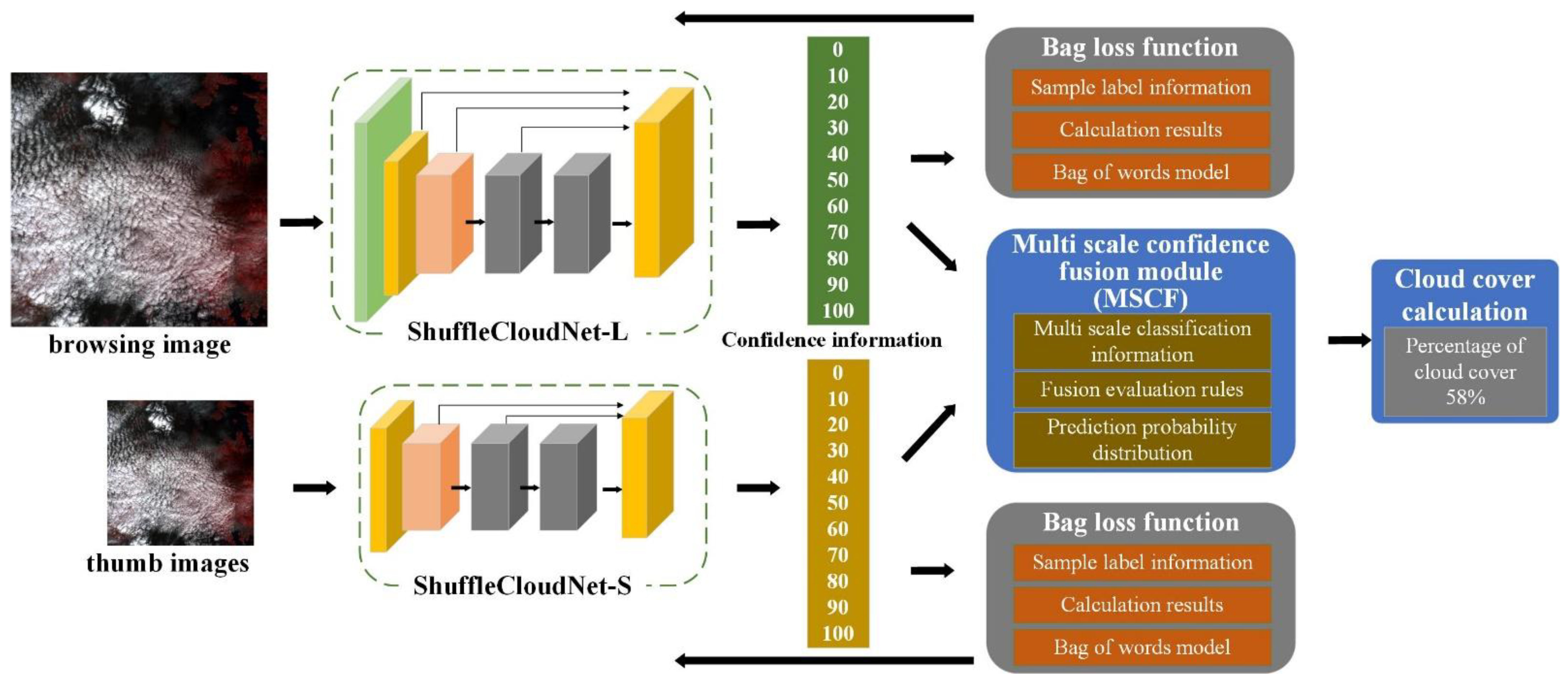
As shown in Figure 2, the L1 and L2 remote-sensing image products include the original remote-sensing image, metadata, RPB data, browsing image, and thumbnail image. Among them, the size of the browsing image is about 1024 × 1024, the size of the thumbnail image is about 60 × 60, and the size of the original image is about 7000 × 7000; metadata is used to describe the satellite number, shooting time, bands and other information of the remote-sensing image product; RPB data have detailed RPC model parameters for image orthorectification. Through observation and analysis, we found that the cloud details described in the thumbnail and browsing images are sufficient to identify the cloud amount. Therefore, we used the thumbnail image and browsing image in the standard remote-sensing image products as the input of the designed neural network. At the same time, the designed neural network also needs two structures to process the thumbnail image and browsing image, respectively, and finally, it uses the fusion structure to fuse the results.

Figure 2.
Structure of cloud-amount calculation based on a composite neural network.
A lightweight neural network model, ShuffleCloudNet, is proposed for the cloud-amount calculation of remote-sensing images. Through feature extraction and training optimization, it can obtain the cloud amount from the browsing image and thumbnail image in the standard data of the remote-sensing image. By analyzing the diversity of clouds and the complexity of backgrounds, a multi-scale confidence fusion module is presented to optimize the calculation performance of cloud amounts under different scales, backgrounds, and cloud types. Furthermore, the bag-of-words loss function is introduced to optimize the training process and to better distinguish complex cloud edges, small clouds, and cloud-like backgrounds. The ShuffleCloudNet framework proposed in this paper is shown in Figure 3 and consists of three main parts: (1) the lightweight backbone networks ShuffleCloudNet-L and ShuffleCloudNet-S; (2) the multi-scale confidence fusion (MSCF) module; and (3) the bag-of-words loss function. In the following, a general overview of the algorithm model is provided first, and then the implementation details of the three key steps within the cloud-amount calculation framework are described in detail.

Figure 3.
Structure of cloud-amount calculation based on composite neural network.
3.1. Model Description
In our investigation, we found that clouds are generally large in scale, greater than 100 m [2,5,6,7,8,9,10,11,12,22,37,38,39]. Hence, cloud-amount calculation using high-resolution remote-sensing images consumes too many computational resources while the accuracy improvement is too limited. Generally, browsing images can be a good way to obtain cloud-amount information from remote-sensing images, and thumbnail images can obtain cloud-amount information from remote-sensing images on a more global scale.
First, the cloud-amount calculation problem of remote-sensing images can be described as the following process. Suppose the remote-sensing image used for cloud-amount calculation is d, and the backbone neural network model is applied to calculate the convolutional features of the remote-sensing image. In general, the more complex the structure of the backbone neural network is, the better its feature-extraction capability and the more robust the semantic representation is. However, if the network size is continuously increased to make its structure complex, then the parameters and computation of the whole network will continuously increase. The most straightforward way to solve such problems is to design lightweight network structures to accomplish the convolutional feature extraction in the cloud-amount calculation, to obtain more efficient and fast computational efficiency. Nevertheless, this operation inevitably ignores the semantic need for deep-level features, which reduces the network’s performance. Thus, contextual and background knowledge feature information are employed to improve and stabilize the model’s computational power and solve this problem. Although some existing methods [19,20,21] have built some context and background extraction units, these models are difficult to adaptively adjust to remote-sensing images from different loads. Moreover, they adopt the more mature but complex neural networks in the field as the backbone network, which also intrinsically contributes to the difficulty in adaptation to remote-sensing processing.
As mentioned above, the purpose of the method in this paper is to design a lightweight and high-accuracy method for cloud-amount calculation. To achieve this goal, we first build a lightweight backbone neural network to extract convolutional features. It should be noted that the backbone neural network contains two parts: the small neural network for extracting the convolutional features of the browsing images from remote-sensing images and the tiny neural network for extracting the convolutional features of the thumbnail images from remote-sensing images. Next, we transform these features into a multi-scale pyramidal feature representation. The details are shown in the following equation:
Here, denotes the features of the obtained multi-scale pyramidal network and indicates the processing operation of the multi-scale feature extraction module. On this basis, MSCF is combined to perform the fusion calculation of the probability distribution of the multi-scale multi-cloud amount to obtain the final cloud-amount calculation results of remote-sensing images.
In this way, MSCF can use background knowledge and fusion rules to perform fusion calculations based on the output individual cloud-amount probabilities, yielding a final output as a cloud-amount result that considers both detailed information and overall features while integrating multiple cloud-amount possibilities.
In the forward inference process, it is already possible to accomplish the related work. However, it is also necessary to fully consider how both the proposed module and the final results can be fed into the training process. Thus, the model can be continuously optimized during the training phase to achieve efficient feature extraction that balances various cloud types and multiple cloud scales. We define a bag-of-words loss function to train the entire network and update the network parameter .
where is the hypothetical hyperparameter space of the search. In this paper, a complete composite neural network model is developed. However, only the core backbone neural network is really needed to enter the training phase, and the other parts are only used for information processing in feedback. As a result, the entire network can be used with maximum efficiency both in the training and testing phases.
3.2. ShuffleCloudNet
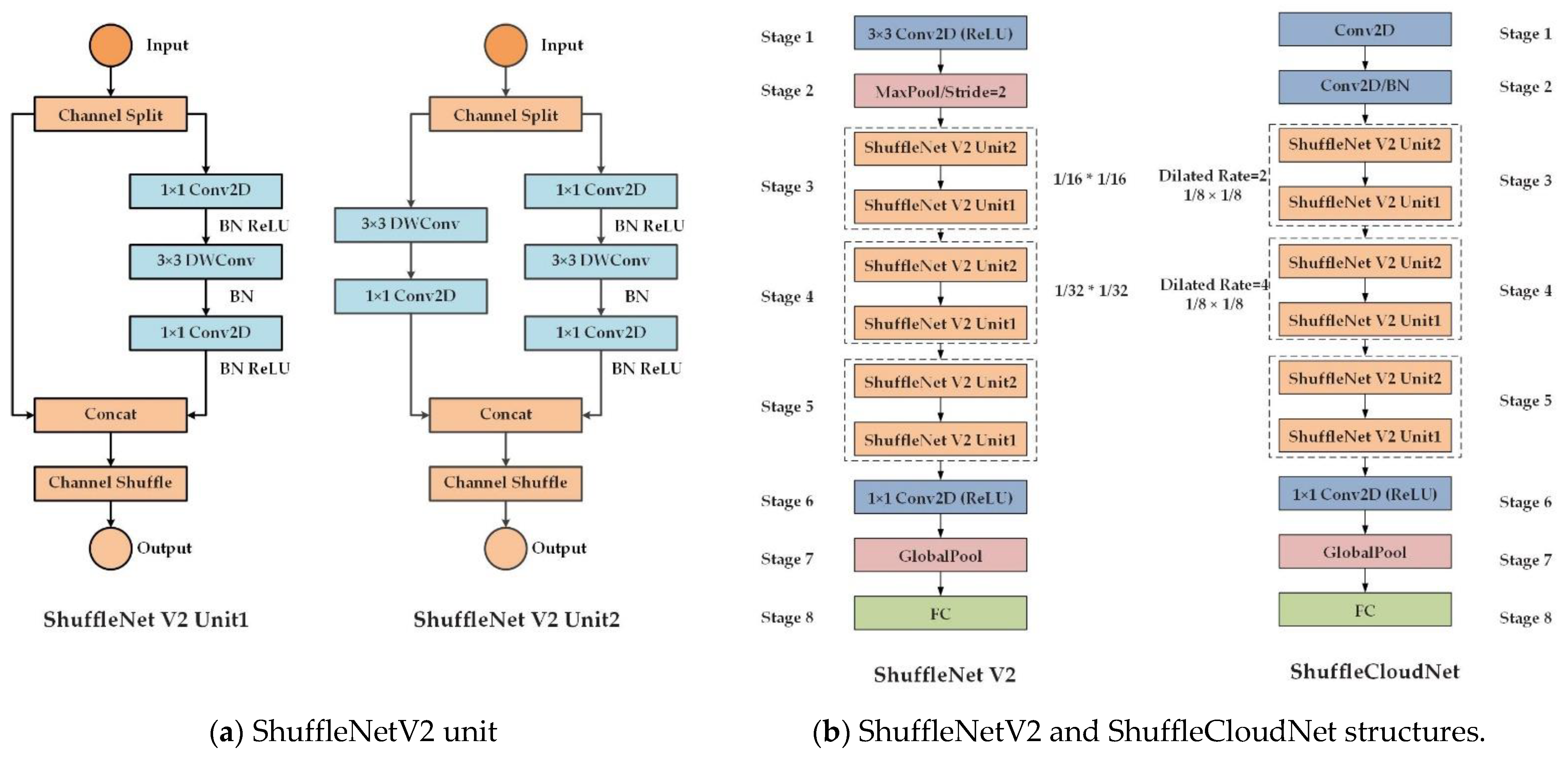
To improve the efficiency of the cloud-amount calculation network as much as possible, we designed ShuffleCloudNet, a lightweight backbone network inspired by ShuffleNetV2. The main units and network structure of ShuffleNetV2 are shown in Figure 4. The original ShuffleNetV2 network uses numerous downsampling operations, which hides many details of the image, and is very disadvantageous to perceiving the cloud amount in the full image distribution of remote-sensing images. For example, many small clouds are difficult to be perceived by the general network and are included in the final cloud-amount calculation results because they occupy few pixels and are easily lost in the neural network convolution operation. If it is possible to pass the high-resolution information of the thumbnail images and the browsing images of remote-sensing images through the model and to ensure that the output information can represent the main content of the input information, then the neural network parameters can be tuned down during the training process thus enabling the network to learn to obtain the basic information of small clouds.
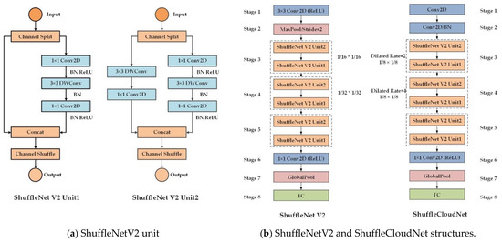
Figure 4.
Diagram of the comparison between ShuffleNet V2 and ShuffleCloudNet network structure.
In the design of neural networks, the most straightforward way to preserve the high-resolution information of the model is to remove the downsampling units from the network directly. However, directly removing the downsampled units reduces the perceptual field of the next layer, which is not conducive to the extraction of global contextual information. Therefore, it is a good choice to adopt the expanded convolutional unit to improve the high-level perceptual field. As shown in Figure 4b, the downsampling modules in stages 1 and 2 of ShuffleNetV2 are replaced with standard convolutional modules that can retain more information. To compensate for the decrease in receptive fields, expansion convolutions with 2 and 4 rates were used in stages 3 and 4, respectively. Different from the 32-fold downsampling of ShuffleNetV2, the model designed in this paper only conducts 8-fold downsampling, which greatly preserves the detailed information. Moreover, there is no change in the parameter number and network layers, which keeps the characteristics of the lightweight network well and provides the basis for subsequent efficient computation of the cloud amount. The features extracted by the backbone network of ShuffleCloudNet retain more detailed information and more overall weak feature information, which is an excellent solution for small-cloud detection and considers the overall information extraction of thin clouds. To ensure the convergence of the proposed model and avoid overfitting, we add a batch normalization layer.
After the backbone neural network model, we add a multi-scale confidence fusion module to improve the support capability of multi-scale information for cloud-amount calculation. By adding the multi-scale confidence fusion module, the CNN can adaptively obtain a more explicit representation of spatial features in remote-sensing images after training. This helps to separate the structural information of similar objects (i.e., clouds and snow) and better capture long-term dependencies. Additionally, this long-term dependency on the model is the main reason the business system of cloud-amount calculation can operate steadily.
3.3. Multi-Scale Confidence Fusion (MSCF) Module
In terms of data sources and different algorithms used in the past, this paper designs a two-way neural network and employs thumbnail images and browsing images as inputs for cloud-amount calculation instead of the original remote-sensing images. This operation reduces the computational workload and can better perceive the cloud distribution at the full scale of remote-sensing images, which is efficient and accurate. However, we found through experiments that due to the different sizes of thumbnail images and browsing images, there are some differences in extracting cloud-amount information. Therefore, we propose the multi-scale confidence fusion module MSCF to effectively balance the effects of inconsistent scale information introduced by the two images.
3.3.1. Multi-Scale Classification Information
To clarify the step characteristics of clouds, we divide the cloud amount into 11 classes, i.e., 0, 10, 20, 30, 40, 50, 60, 70, 80, 90, and 100, which makes it easier to distinguish different cloud amounts for classification networks. If the cloud amount is only split into two categories by 50, it may lead to an extremely rapid decrease in model convergence.
3.3.2. Rules for Fusion Evaluation
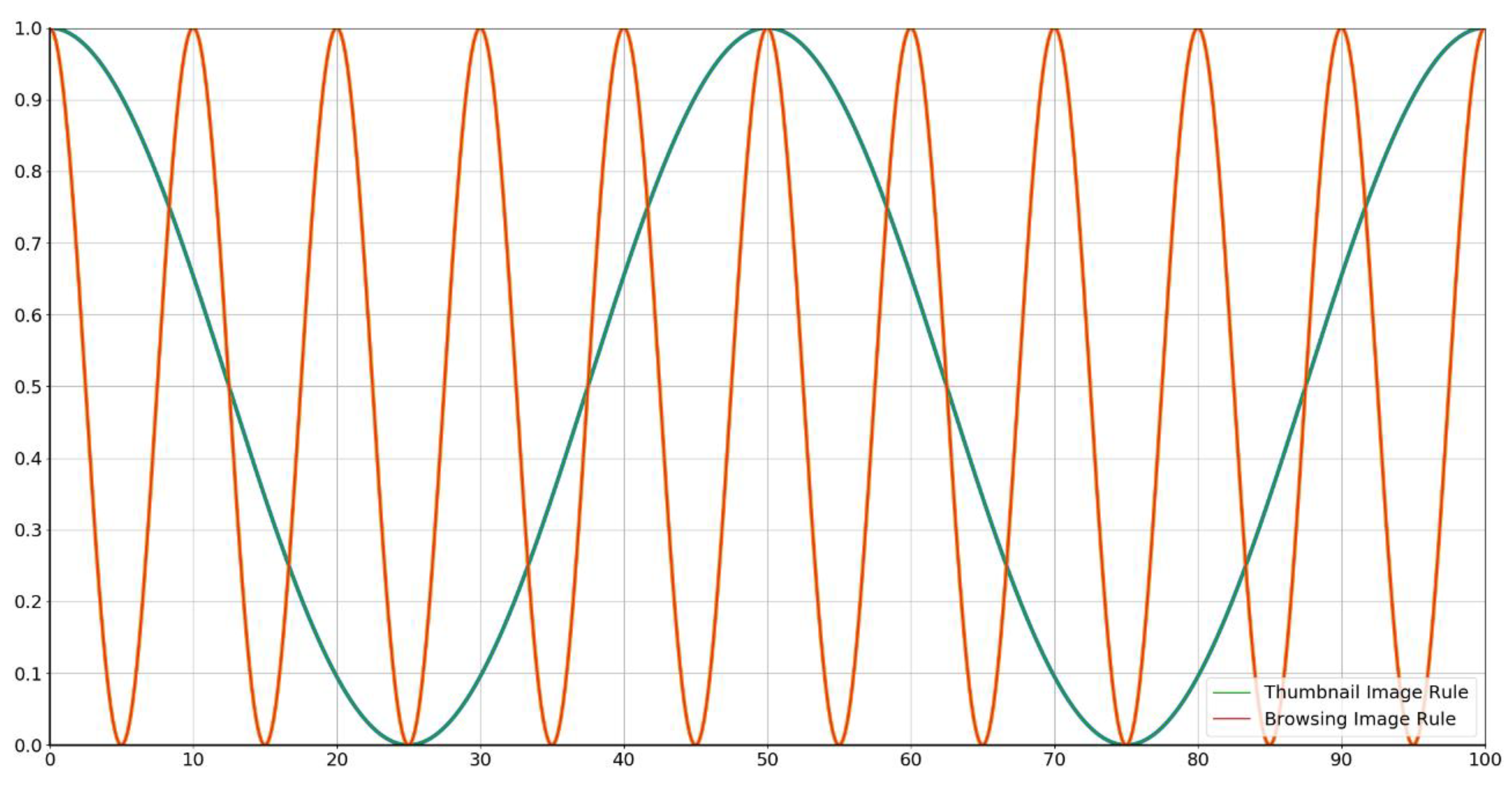
To accommodate the different granularities of detailed cloud information reflected in both the thumbnail image and the browsing image in remote-sensing images, we set up a fusion-evaluation rule. The main principle of this fusion-evaluation rule is that the thumbnail image is faster and more efficient in distinguishing large-scale cloud amounts. For example, it more easily distinguishes cloud amounts of 0, 50, 80, and 100. However, when we distinguish the 20, 30, and 40 cloud amounts in the close range, we mainly refer to the classification results provided by the browsing image.
The rules we set can be presented by two Gaussian curves, as shown in Figure 5.
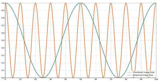
Figure 5.
Diagram of the fusion-evaluation rules for the composite neural network.
3.3.3. Probability Distribution Prediction
The predicted probability of the obtained cloud-amount calculation is a list of probability predictions for each cloud-amount phase, as represented in Table 1.

Table 1.
Probability distribution table of cloud-amount calculation.
According to the probability distribution, several adjacent probabilities of the cloud amount with the highest probability are accumulated. The specific process is as follows:
- Find the cloud-amount class with the highest probability in the output of the classification result, denoted as , corresponding to the probability as , where 0 ≤ n ≤ 10 is a natural number;
- Determine the selection number M of the adjacent cloud-amount levels for the highest cloud-amount level;
- Normalize the cloud-amount level probability, , where ;
- The final cloud amount is .
Several adjacent cloud-amount levels are selected for calculation and relevant experiments. M is set to 0, 2, 4, 6, and 8. Cloud-amount prediction is performed using the above steps and compared with the real values, and the final experimental results are statistically analyzed with an error of less than 5. Among them, 55 samples are selected for this statistical experiment, and their real cloud-amount levels are uniformly distributed from 0 to 100. The experimental results show that the selection of M = 2 is most suitable. The specific experimental situation is shown in Table 2.

Table 2.
Table of experimental results for cloud-amount level selection.
4. Experimental Results
In this section, we focus on showing the comparative experimental results of the proposed ShuffleCloudNet on the dataset CTI_RSCloud and other publicly available datasets (GF-1 WFV [37] and AIR-CD [38]). First, we briefly introduce each dataset; then, we preprocess all datasets according to the requirements to meet our experimental requirements. Among them, we focus on preparing the cloud-amount calculation dataset CTI_RSCloud for remote sensing. Next, we demonstrate the ablation experiments of key components of ShuffleCloudNet. Finally, the overall performance of the model is analyzed quantitatively and qualitatively.
4.1. Experimental Data
To quantitatively evaluate the performance of ShuffleCloudNet, we conducted experiments on three datasets of cloud detection and cloud-amount calculation for optical remote-sensing images. The first is our own constructed dataset CTI_RSCloud for the cloud-amount calculation of remote-sensing images; the second is the cloud-detection dataset of remote-sensing images of GF-1 WFV; and the third is the AIR-CD dataset composed of remote-sensing images of GF-2.
- CTI_RSCloud: This mainly includes 1829 browsing images of remote-sensing images and an equal number of thumbnail images, with images mainly from GF-1, GF-2, ZY series, etc.
- GF-1 WFV: This was created by the SENDIMAGE lab. The dataset contains 108 complete scenes at level 2A, where all masks are labeled with cloud, cloud shadow, clear sky, and non-value pixels. The spatial resolution of the dataset is 16 m and consists of one NIR band and three visible bands. Since our study concentrates on detecting cloud pixels, all other classes of masks are set to background pixels (i.e., non-cloud pixels). Specifically, the cloud shadows, clear sky, and non-value pixels in the original masks are set to 0, and the cloud pixels are set to 1.
- AIR-CD: This is based on GF-2 high resolution, which includes 34 complete scenes collected by GF-2 satellite from different regions of China between February 2017 and November 2017. AIR-CD is one of the earliest publicly available cloud-detection datasets of remote-sensing images collected from GF-2 satellites. In addition, the scenes in AIR-CD are more complex than in previous datasets, making it more challenging to achieve high-accuracy cloud detection and cloud-amount calculation. The dataset contains various land-cover types, including urban, wilderness, snow, and forest. The dataset consists of near-infrared and visible bands with a spatial resolution of 4 m and a size of 7300 × 6908 pixels. Considering the radiation difference between PMS1 and PMS2 sensors in the GF-2 satellite imaging system, the scenes of both sensors are used as experimental data to ensure the generalization ability of the model.
4.2. Data Preprocessing
To obtain training and test data adapted to the model, we conducted relevant preprocessing for the CTI_RSCloud, GF-1 WFV, and AIR-CD datasets, respectively.
- CTI_RSCloud: The main elements of preprocessing are data filtering, cloud-amount level classification, cloud-amount judgment rules, sample annotation, etc.
- Selection of remote-sensing images
To find the characteristics of remote-sensing image clouds more objectively, we try to filter remote-sensing images according to the season, month, region, and satellite for balanced interpretation and translation. Presently, it includes the remote-sensing data of four seasons—the spring, summer, autumn, and winter, January to December; four continents—Asia, Europe, Africa, and America; and satellites, such as GF1, GF2, ZY, and CB04. Additionally, at the same level, we selected as many different types of cloud amounts as possible.
- Cloud-amount level division
To clarify the step characteristics of the cloud amount, we divide the cloud amount into 11 levels, i.e., 0, 10, 20, 30, 40, 50, 60, 70, 80, 90, and 100.
- Cloud-amount interpretation rules
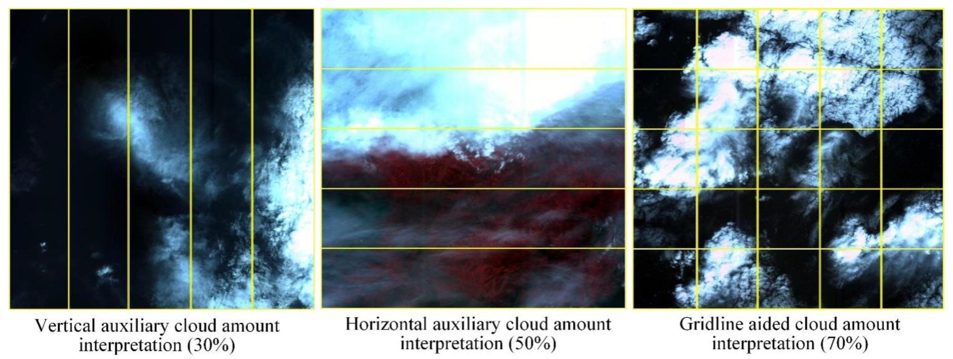
In the manual interpretation of the labeled cloud-amount calculation samples, three rules, or principles, are followed. (i) The principle of balancing multiple types of clouds, i.e., thick clouds, thin clouds, etc. Therefore, when we manually collect and sort remote-sensing images, we generally control the proportion of thin clouds, thick clouds, and point clouds at each cloud level. For example, 35 thin clouds, 39 thick clouds, 25 thin–thick clouds, and 18 others are included in the cloud-amount calculation samples of remote-sensing images with a level of 50. (ii) The principle of grid-assisted interpretation, using horizontal, vertical, and grid lines to assist in cloud-amount division. (iii) The principle of upward rounding, considering the complexity of cloud-amount calculation and the enhancement effect of human visual ability. Therefore, after interpreting the cloud amount of a remote-sensing image, it is directly rounded upward; for example, 46 is rounded up and grouped into 50. Figure 6 shows a schematic diagram of cloud-amount division with the aid of horizontal, vertical, and grid lines. If the cloud amount is simple and the horizontal distribution is large, the horizontal line shall be used for auxiliary interpretation. If the vertical distribution angle is large, the vertical line shall be used for auxiliary interpretation. Considering the efficiency and the cloud-amount level of 0–10 set by us, the cloud amount can be divided into five horizontal lines and five vertical lines. If the cloud-amount distribution is complex, the 5 × 5 vertical and horizontal lines shall be used to intersect.

Figure 6.
Schematic diagram of grid cloud-amount calculation.
Finally, through the above operations, the remote sensing cloud-amount calculation dataset CTI_RSCloud is obtained, which contains 225 cloud-free samples, 449 10-rank samples, 192 20-rank samples, 158 30-rank samples, 145 40-rank samples, 117 50-rank samples, 106 60-rank samples, 110 70-rank samples, 106 80-rank samples, 108 90-rank samples, and 113 100-rank samples, with a total of 1829 samples.
- 2.
- GF-1 WFV and AIR-CD
Both GF-1 WFV and AIR-CD are raw data from remote-sensing images, which need to be changed into the size of the browsing image and thumbnail image and given the corresponding cloud-amount level labels. In calculating the cloud-amount levels for the above two datasets, the detailed cloud-amount percentage calculation is performed using the already-obtained cloud-detection masks and then rounded upwards to obtain the cloud-amount level label. Among them, GF-1 WFV obtained 6 cloud-free samples, 32 10-grade samples, 19 20-grade samples, 17 30-grade samples, 6 40-grade samples, 6 50-grade samples, 4 60-grade samples, 4 70-grade samples, 7 80-grade samples, 5 90-grade samples, and 0 100-grade samples, for a total of 100 samples. AIR-CD obtained 10 cloud-free samples, 11 10-grade samples, 7 20-grade samples, 2 30-grade samples, 2 40-grade samples, 1 50-grade sample, 0 60-grade samples, 0 70-grade samples, 0 80-grade samples, 1 90-grade sample, and 0 100-grade samples, for a total of 34 samples.
4.3. Implemental Details
4.3.1. Evaluation Metrics
To evaluate the performance of different methods in the cloud-amount calculation of remote-sensing images, four widely used quantitative metrics, namely precision (top 3), precision (top 5), overall parameters of the model (Params), and inference runtime, are utilized. It should be noted that precision (top 3) and precision (top 5) are utilized as classification accuracy metrics—and the larger the value, the higher the accuracy; Params and the inference runtime are considered efficiency metrics, where smaller is usually better.
4.3.2. Comparative Models
The model proposed in this paper is compared with typical CNN-based cloud-amount calculation methods, including three classic lightweight neural network architectures, MobileNetV2, SqueezeNet, and ShuffleNetV2. MobileNetV2 is a classification backbone network proposed by the Google team in 2018, which is an improved version of MobileNet with the addition of Linear Bottleneck and Inverted Residual. SqueezeNet was proposed in the same period as MobileNet, and its core idea is a fire module that adopts the structure of squeeze and expand, thus improving the training efficiency and reducing the parameter number. ShuffleNetV2, guided by four design principles of lightweight networks and based on ShuffleNetV1, introduces the idea of Channel Split and proposes a novel convolutional block architecture, a practical network architecture that can be deployed industrially.
Because we have not used deep neural networks to directly calculate the cloud cover of remote-sensing images, most algorithms have cloud detection as the ultimate goal. Therefore, we selected three cloud-detection algorithms based on deep neural networks as comparison algorithms and selected their backbone networks as the main comparison models to join in the comparison experiment. They are the backbone networks of MFFSNet (improved Resnet101), MSCFF (CBRR module combination), and CDNet (improved Resnet50). At the same time, to ensure that the three network models can reach the highest level, we fully trained and taught the three models the cloud-detection dataset GF-1 WFV and AIR-CD. Later, along with other comparison models, the cloud-amount calculation data set CTI_RSCloud was trained.
Since the lightweight backbone network of the proposed method is mainly redesigned based on the ShuffleNetV2, we also analyzed ShuffleCloudNet in the ablation studies.
4.3.3. Experimental Setup
All models in the experiments are trained on the training set and tested on the corresponding test set, where samples obtained from GF-1 WFV and AIR-CD preprocessing are all used for testing. All models use RGB images as input, and only the cloud amount is calculated without detecting the specific location of the clouds. In the training process, we classify the browsing and thumbnail images as separate training sets in ShuffleCloudNet-L and ShuffleCloudNet-S. Data augmentation is conducted by flipping horizontally and rotating at a specific angle. The models are optimized using the Adam algorithm. In particular, we set the hyperparameters β1 = 0.9, β2 = 0.999, and ε = 10−8. The initial learning rate is set to 1 × 10⁻⁴ and reduced by half every 10 epochs for a total of 300 epochs. All experiments are implemented in the Pytorch framework with an NVIDIA RTX 3090 GPU.
4.4. Ablation Experiments
To better validate the superiority of the proposed method, we conducted ablation studies in ShuffleCloudNet-L, ShuffleCloudNet-S, MSCF, and BW loss.
- Effect of ShuffleCloudNet-L and ShuffleCloudNet-S
We conducted the experiments using ShuffleNetV2, ShuffleCloudNet-L, ShuffleCloudNet-S, and ShuffleCloudNet, respectively. The corresponding results in this ablation experiment are shown in Table 3. It can be seen that there is a certain loss of accuracy or time consumption in the cloud-amount calculation results when using ShuffleNetV2, ShuffleCloudNet-L, and ShuffleCloudNet-S only. Additionally, the combination of ShuffleCloudNet-L and ShuffleCloudNet-S meets the lower time requirement with the highest accuracy guaranteed.

Table 3.
Effects of the ShuffleNet module with different combinations on the CTI_RSCloud dataset.
- 2.
- Effect of MSCF
To evaluate the performance of the MSCF module, we take “ShuffleCloudNet-L+ShuffleCloudNet-S+RN” as the benchmark so that the whole network does not consider the feature pyramid mechanism. Furthermore, the MSCF module is added to achieve the final result. As shown in Table 4, adding the MSCF module significantly improves the accuracy of the cloud-amount calculation.

Table 4.
Effects of the MSCF module on the CTI_RSCloud dataset.
- 3.
- Effect of BW loss
To verify the effect of the loss function, we train the network in two ways. Formally, the first method is “BCE loss” (i.e., training with BCE loss), and the other method is “BW loss” (i.e., training with BW loss). As shown in Figure 7, the network model trained by BW loss has better results in processing remote-sensing images that contain thin clouds and debris clouds, which are more difficult to calculate. Table 5 shows the corresponding quantitative results, and BW loss achieves good results in precision (top3) and precision (top5) accuracy metrics. The results show that BW loss can guide the network to learn strong semantics and help optimize the stability and representativeness of cloud-amount calculation.

Figure 7.
Results with BW loss compared to BCE loss. (a) is an example of cloud amount calculation result of remote sensing image of speckled cloud. (b) is an example of cloud amount calculation results of thin cloud remote sensing image. (c) is an example of cloud amount calculation result of remote sensing image of thin cloud and thick cloud mixture. (d) is an example of cloud amount calculation results of remote sensing images of thin clouds and speckled clouds.

Table 5.
Effects of different loss functions on the CTI_RSCloud dataset.
4.5. Comparison with State-of-the-Art Methods
- Quantitative analysis
Table 6 shows the performance of our ShuffleCloudNet and other state-of-the-art methods on CTI_RSCloud, AIR-CD, and GF-1 WFV datasets. Considering the parameters and multiple additions, ShuffleCloudNet has a significant advantage over other models in terms of efficiency. Our method produces accuracies of 82.85 (precision (top 3)), 92.56 (precision (top 5)), 97.06 (precision (top 3)), 100.00 (precision (top 5)), 72.74 (precision (top 3)), and 83.02 (precision (top 5)), which reaches the accuracy of the complex cloud detection and computation model.

Table 6.
Comparison of the performance of different methods for cloud-amount calculation.
In Table 7, we evaluate the inference runtimes of these networks. The runtimes are calculated based on input data of 1024 × 1024 pixels, respectively. The runtime of ShuffleCloudNet is much lower than other cloud-detection methods. Especially for large data inputs, the advantage is more obvious. The runtime can be used to intuitively evaluate the model efficiency (i.e., complexity), which mainly depends on the parameters and computations (multiple additions) of the model. The smaller the parameters and multiple additions, the more efficient the model is and the shorter the inference runtime. Since the runtime also depends on memory access, some comparison methods seem very close to this metric. In our further work, we will optimize the model structure of ShuffleCloudNet to further reduce the inference runtime.

Table 7.
Comparison of the parameters and the inference runtime of different methods of cloud detection.
- 2.
- Qualitative analysis
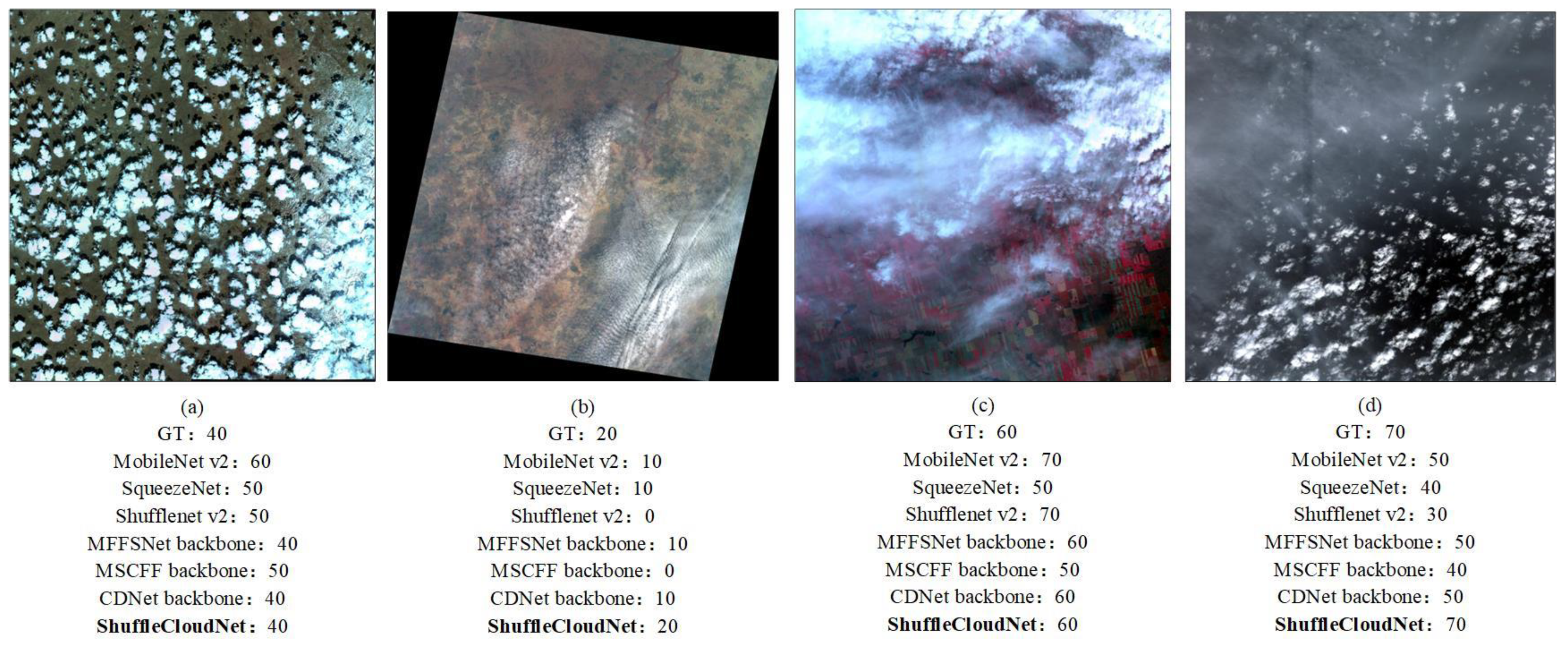
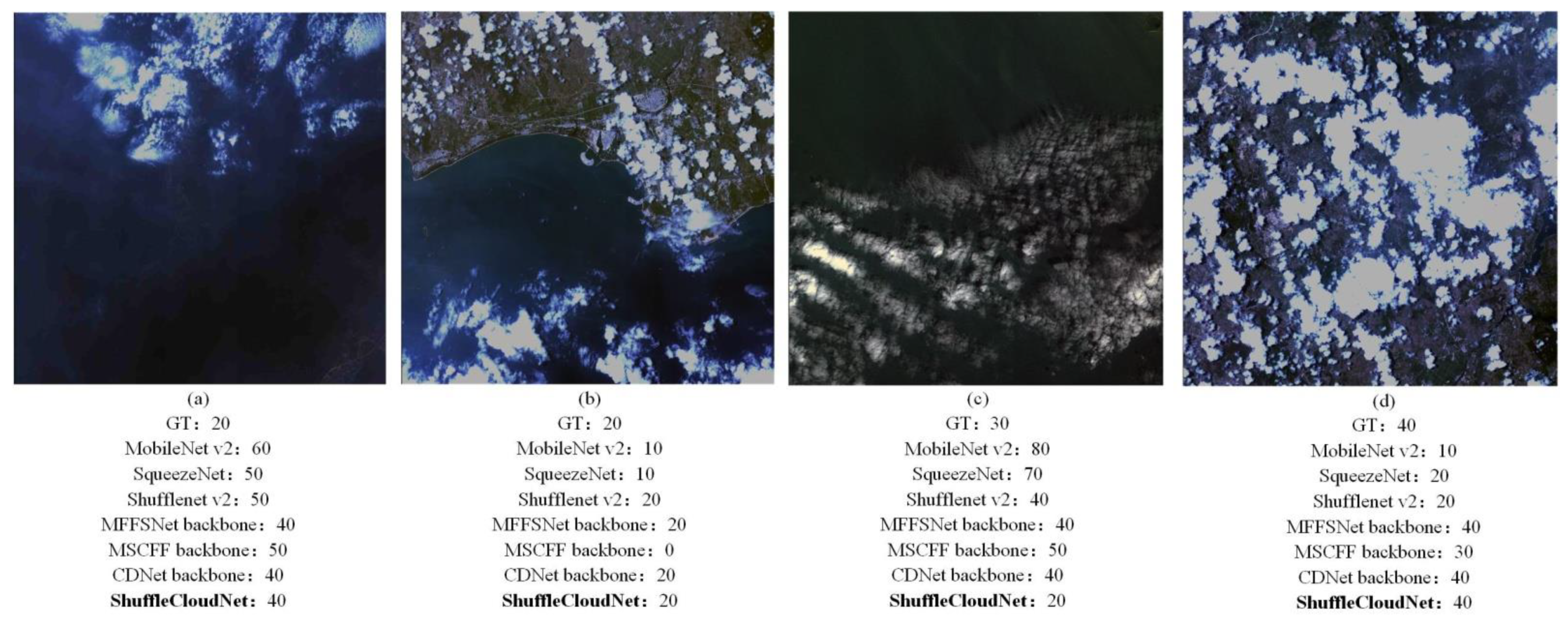
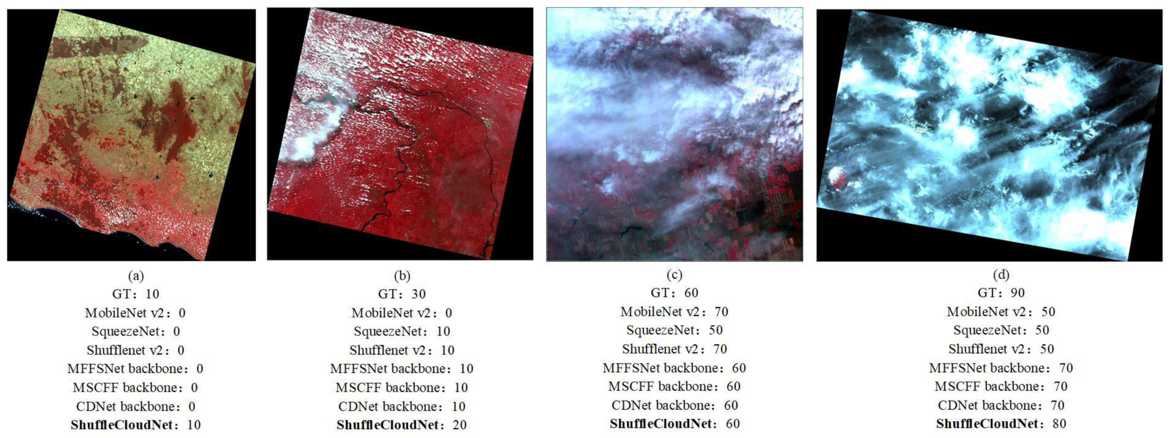
Figure 8, Figure 9 and Figure 10 compare different methods on CTI_RSCloud, AIR-CD, and GF-1 WFV datasets. We select some representative image-visualization results, including thin clouds, small clouds, and the coexistence of clouds and snow. The results show that our method is significantly superior to others. Specifically, the MobileNet method generates more misclassification results in snowy regions. Due to the introduction of a multi-scale feature-extraction mechanism, SqueezeNet and ShuffleNet are significantly improved. MFFSNet and CDNet backbones use improved Resnet 101 and Resnet50, respectively, which have strong feature-extraction and convergence abilities and cloud-computing effects superior to lightweight models such as MobileNet. However, the runtime of the MFFSNet backbone and CDNet backbone is long, and they do not meet the application scenarios of high time efficiency and low resources. When the MSCFF backbone loses its multi-scale fusion module, which is the most characteristic of a cloud-detection network, its cloud-computing effect is relatively general. Unlike them, ShuffleCloudNet has a lightweight multi-scale architecture, which greatly reduces the total number of parameters and calculations. By implementing the MSCF module and BW loss, cloud and snow pixels with similar colors can be effectively distinguished, and the results of the cloud-amount calculation are more accurate. Therefore, our ShuffleCloudNet has an excellent generalization capability for the cloud-amount calculation task of optical remote-sensing images.

Figure 8.
Test example diagram of CTI_RSCloud dataset. (a) is an example of cloud amount calculation result of remote sensing image of speckled cloud. (b) is an example of cloud amount calculation results of thin cloud remote sensing image. (c) is an example of cloud amount calculation result of remote sensing image of thin cloud and thick cloud mixture. (d) is an example of cloud amount calculation results of remote sensing images of thin clouds and speckled clouds.

Figure 9.
Test example diagram of AIR-CD dataset. (a) is an example of cloud amount calculation result of remote sensing image of thin cloud and thick cloud mixture. (b) is an example of the cloud amount calculation result of remote sensing image in the sea land scene. (c) is an example of the cloud amount calculation result of remote sensing image in the evening time. (d) is an example of cloud amount calculation result of remote sensing image of speckled cloud.

Figure 10.
Test example diagram of GF-1 WFV dataset. (a) is an example of cloud amount calculation results of remote sensing image with a few clouds. (b) is an example of cloud amount calculation results of remote sensing image of large-scale speckled cloud. (c) is an example of cloud amount calculation result of remote sensing image of thin cloud and thick cloud mixture. (d) is an example of cloud amount calculation results of remote sensing image with multi type cloud mixture.
4.6. Limitations
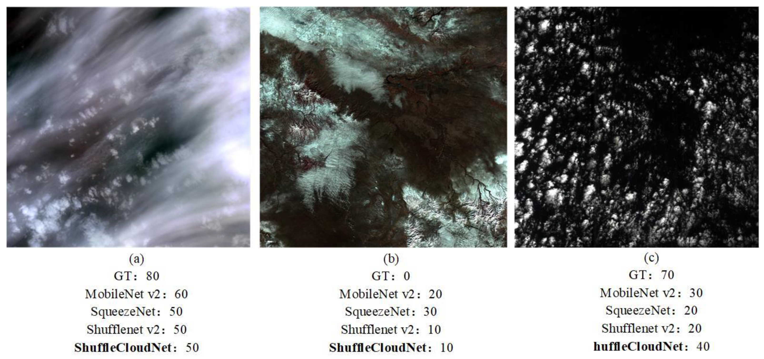
ShuffleCloudNet can achieve decent cloud-amount calculation in many difficult scenarios but still suffers from some errors in cases such as thin cloud, fog, ice, and mixing of snow clouds. Thin clouds are usually visually recognizable. When the surface below is faintly visible, most thin clouds appear almost the same as subsurface objects. Thus, the problem of thin clouds missing in the calculation results easily occurs. Snow and ice have similar characteristics to clouds in some cases and are also easily misidentified by the human eye. Figure 11 shows three cases of incorrectly calculated cloud amounts. The last case (Figure 11c) has poor cloud-amount calculation, mainly due to the information loss after 16-bit to 8-bit image conversion. In the future, we will optimize the model to further improve the robustness of the proposed method in situations such as thin clouds, ice, and snow.

Figure 11.
Example diagram of poor cloud-amount calculation results. (a) is an example of the cloud amount calculation result of remote sensing image with thin cloud covering thick cloud. (b) is an example of cloud amount calculation result of remote sensing image of ice snow cloud mixture. (c) is an example of the cloud amount calculation result of remote sensing image at low contrast in the evening.
5. Discussion
From the precision (top 3) and precision (top 5) values in Table 3, it can be seen that the improved ShuffleCloudNet achieves an accuracy of about 10 percentage points higher than ShuffleNetV2 on the CTI_RSCloud dataset; of course, due to the model design, its parameters are also larger than ShuffleNetV2 by a factor of two. As can be seen from Table 4, the design and addition of the MSCF module increased the precision (top 3) and precision (top 5) values by 5% and 3%, respectively. Figure 7 and Table 5 show the role of the BW loss function. The trained model mainly improves the cloudiness calculation capability of speckle clouds, thin clouds, and their combination. The test results of the three datasets in Table 6 and Figure 8, Figure 9 and Figure 10 show that the proposed ShuffleCloudNet model has the best performance in remote-sensing cloud computing and has a small number of parameters. In Table 7, we compare it with the current best cloud-detection models and find that its precision (top 3) is 100% (our model is 97.06), but the runtime and parameters are far greater than the proposed ShuffleCloudNet. The amount of parameters is 4 to 7 times that of ShuffleCloudNet, and the runtime is 200 times that of ShuffleCloudNet. However, the experiment also clarified the areas where future research is needed to improve it. First of all, the directivity of the model in the cloud-cover calculation is not clear enough. Therefore, there are cases where the calculation of thin clouds and fog is inaccurate, and ice and snow are included in cloud cover. With data reaching the tens of millions, there are still many cases. Another area of improvement is how to quickly obtain the browsing and thumbnail images of remote-sensing images under in-orbit deployment and quickly update the model. In summary, we will continue to improve the model, fully considering the current popular lightweight model structures, to obtain a more stable and precise classification calculation effect.
6. Conclusions
In this paper, we propose an effective cloud-amount calculation method, named ShuffleCloudNet, for optical remote-sensing images. Compared with the results of currently published lightweight cloud-amount calculations, the accuracy of ShuffleCloudNet can attain even better performance. An MSCF module is utilized in our method to extract multi-scale features adaptively based on the shape and size features of clouds. Moreover, we have designed ShuffleCloudNet-L for the feature extraction of browsing images and ShuffleCloudNet-S for the feature extraction of thumbnail images in remote-sensing images. Furthermore, a novel BW loss function is also constructed, leading the network to pay more attention to the pixels near the cloud boundary. To better test the method’s effectiveness in this paper, we built our own remote-sensing cloud-amount calculation dataset, CTI_RSCloud. The experiments based on CTI_RSCloud, AIR-CD, and GF-1 WFV datasets demonstrate that our method outperforms the baseline method and achieves better efficiency than the existing algorithms. In the future, we will try to optimize the model structure to improve the computational performance for situations such as thin clouds, snow, and ice. Moreover, we will explore model designs based on specific onboard computing platforms (e.g., FPGAs and ASICs) to further improve operational efficiency.
Author Contributions
Conceptualization, G.W. and Z.L.; methodology, G.W.; software, G.W.; validation, G.W. and Z.L.; formal analysis, G.W. and Z.L.; investigation, G.W.; resources, G.W.; data curation, G.W.; writing—original draft preparation, G.W.; writing—review and editing, Z.L.; visualization, G.W.; supervision, P.W.; project administration, G.W.; funding acquisition, G.W. All authors have read and agreed to the published version of the manuscript.
Funding
This research was funded by the Key Program National Natural Science Foundation of China, grant number U20B2064.
Data Availability Statement
The dataset used in this article will be published on Baidu Netdisk.
Acknowledgments
We thank Jinyong Chen for revising and improving the method proposed in this paper and Min Wang for his contribution to the quantitative calculation of this paper. We also thank Wei Fu for financially supporting this article.
Conflicts of Interest
The authors declare no conflict of interest.
References
- Zhang, Y.; Rossow, W.B.; Lacis, A.A.; Oinas, V.; Mishchenko, M.I. Calculation of radiative fluxes from the surface to top of atmosphere based on ISCCP and other global data sets: Refinements of the radiative transfer model and the input data. J. Geophys. Res. Atmos. 2004, 109, D19105. [Google Scholar] [CrossRef]
- Lu, D. Detection and substitution of clouds/hazes and their cast shadows on IKONOS images. Int. J. Remote Sens. 2007, 28, 4027–4035. [Google Scholar] [CrossRef]
- Mackie, S.; Merchant, C.J.; Embury, O.; Francis, P. Generalized Bayesian cloud detection for satellite imagery. Part 1: Technique and validation for night-time imagery over land and sea. Int. J. Remote Sens. 2010, 31, 2595–2621. [Google Scholar] [CrossRef]
- He, Q.-J. A daytime cloud detection algorithm for FY-3A/VIRR data. Int. J. Remote Sens. 2011, 32, 6811–6822. [Google Scholar] [CrossRef]
- Marais, I.V.Z.; Preez, J.A.D.; Steyn, W.H. An optimal image transform for threshold-based cloud detection using heteroscedastic discriminant analysis. Int. J. Remote Sens. 2011, 32, 1713–1729. [Google Scholar] [CrossRef]
- Han, Y.; Kim, B.; Kim, Y.; Lee, W.H. Automatic cloud detection for high spatial resolution multi-temporal images. Remote Sens. Lett. 2014, 5, 601–608. [Google Scholar] [CrossRef]
- Lin, C.H.; Lin, B.Y.; Lee, K.Y.; Chen, Y.C. Radiometric normalization and cloud detection of optical satellite images using invariant pixels. ISPRS J. Photogramm. Remote Sens. 2015, 106, 107–117. [Google Scholar] [CrossRef]
- Adrian, F. Cloud and Cloud-Shadow Detection in SPOT5 HRG Imagery with Automated Morphological Feature Extraction. Remote Sens. 2014, 6, 776–800. [Google Scholar]
- Bai, T.; Li, D.; Sun, K.; Chen, Y.; Li, W. Cloud Detection for High-Resolution Satellite Imagery Using Machine Learning and Multi-Feature Fusion. Remote Sens. 2016, 8, 715. [Google Scholar] [CrossRef]
- Wieland, M.; Li, Y.; Martinis, S. Multi-sensor cloud and cloud shadow segmentation with a convolutional neural network. Remote Sens. Environ. 2019, 230, 111203. [Google Scholar] [CrossRef]
- Tian, M.; Chen, H.; Liu, G. Cloud Detection and Classification for S-NPP FSR CRIS Data Using Supervised Machine Learning. In Proceedings of the IGARSS 2019—2019 IEEE International Geoscience and Remote Sensing Symposium, Yokohama, Japan, 28 July–2 August 2019. [Google Scholar]
- Ji, S.; Dai, P.; Lu, M.; Zhang, Y. Simultaneous Cloud Detection and Removal From Bitemporal Remote Sensing Images Using Cascade Convolutional Neural Networks. IEEE Trans. Geosci. Remote Sens. 2020, 59, 732–748. [Google Scholar] [CrossRef]
- Sudhakaran, S.; Lanz, O. Convolutional Long Short-Term Memory Networks for Recognizing First Person Interactions. In Proceedings of the IEEE International Conference on Computer Vision Workshop, Venice, Italy, 22–29 October 2017. [Google Scholar]
- Jeppesen, J.H.; Jacobsen, R.H.; Inceoglu, F.; Toftegaard, T.S. A cloud detection algorithm for satellite imagery based on deep learning. Remote Sens. Environ. 2019, 229, 247–259. [Google Scholar] [CrossRef]
- Xie, W.; Yang, J.; Li, Y.; Lei, J.; Zhong, J.; Li, J. Discriminative feature learning constrained unsupervised network for cloud detection in remote sensing imagery. Remote Sens. 2020, 12, 456. [Google Scholar] [CrossRef]
- Dai, P.; Ji, S.; Zhang, Y. Gated convolutional networks for cloud removal from bi-temporal remote sensing images. Remote Sens. 2020, 12, 3427. [Google Scholar] [CrossRef]
- Li, X.; Zheng, H.; Han, C.; Zheng, W.; Chen, H.; Jing, Y.; Dong, K. SFRS-net: A cloud-detection method based on deep convolutional neural networks for GF-1 remote-sensing images. Remote Sens. 2021, 13, 2910. [Google Scholar] [CrossRef]
- Ma, N.; Sun, L.; Zhou, C.; He, Y. Cloud detection algorithm for multi-satellite remote sensing imagery based on a spectral library and 1D convolutional neural network. Remote Sens. 2021, 13, 3319. [Google Scholar] [CrossRef]
- Xie, F.; Shi, M.; Shi, Z.; Yin, J.; Zhao, D. Multilevel Cloud Detection in Remote Sensing Images Based on Deep Learning. IEEE J. Sel. Top. Appl. Earth Obs. Remote Sens. 2017, 10, 3631–3640. [Google Scholar] [CrossRef]
- Li, Z.; Shen, H.; Cheng, Q.; Liu, Y.; You, S.; He, Z. Deep learning based cloud detection for medium and high resolution remote sensing images of different sensors. ISPRS J. Photogramm. Remote Sens. 2019, 150, 197–212. [Google Scholar] [CrossRef]
- Shao, Z.; Pan, Y.; Diao, C.; Cai, J. Cloud Detection in Remote Sensing Images Based on Multiscale Features-Convolutional Neural Network. IEEE Trans. Geosci. Remote Sens. 2019, 57, 4062–4076. [Google Scholar] [CrossRef]
- Yang, J.; Guo, J.; Yue, H.; Liu, Z.; Hu, H.; Li, K. CDnet: CNN-Based Cloud Detection for Remote Sensing Imagery. IEEE Trans. Geosci. Remote Sens. 2019, 57, 6195–6211. [Google Scholar] [CrossRef]
- Mohajerani, S.; Krammer, T.A.; Saeedi, P. Cloud Detection Algorithm for Remote Sensing Images Using Fully Convolutional Neural Networks. In Proceedings of the 2018 IEEE 20th International Workshop on Multimedia Signal Processing (MMSP), Vancouver, BC, Canada, 29–31 August 2018. [Google Scholar]
- Howard, A.G.; Zhu, M.; Chen, B.; Kalenichenko, D.; Wang, W.; Weyand, T.; Andreetto, M.; Adam, H. MobileNets: Efficient Convolutional Neural Networks for Mobile Vision Applications. arXiv 2017, arXiv:1704.04861. [Google Scholar]
- Sandler, M.; Howard, A.; Zhu, M.; Zhmoginov, A.; Chen, L.C. MobileNetV2: Inverted Residuals and Linear Bottlenecks. In Proceedings of the 2018 IEEE/CVF Conference on Computer Vision and Pattern Recognition (CVPR), Salt Lake City, UT, USA, 18–23 June 2018. [Google Scholar]
- Howard, A.; Sandler, M.; Chu, G.; Chen, L.-C.; Chen, B.; Tan, M.; Wang, W.; Zhu, Y.; Pang, R.; Vasudevan, V. Searching for mobilenetv3. In Proceedings of the IEEE/CVF International Conference on Computer Vision, Seoul, Korea, 27 October–2 November 2019; pp. 1314–1324. [Google Scholar]
- Iandola, F.N.; Han, S.; Moskewicz, M.W.; Ashraf, K.; Dally, W.J.; Keutzer, K. SqueezeNet: AlexNet-level accuracy with 50x fewer parameters and <0.5 MB model size. arXiv 2016, arXiv:1602.07360. [Google Scholar]
- Zhang, X.; Zhou, X.; Lin, M.; Sun, J. ShuffleNet: An Extremely Efficient Convolutional Neural Network for Mobile Devices. In Proceedings of the 2018 IEEE/CVF Conference on Computer Vision and Pattern Recognition (CVPR), Salt Lake City, UT, USA, 18–23 June 2018. [Google Scholar]
- Ma, N.; Zhang, X.; Zheng, H.-T.; Sun, J. ShuffleNet V2: Practical Guidelines for Efficient CNN Architecture Design. In Proceedings of the European Conference on Computer Vision (ECCV); Springer: Cham, Switzerland, 2018; pp. 122–138. [Google Scholar]
- Xia, Y.; Wang, J. A dual neural network for kinematic control of redundant robot manipulators. IEEE Trans. Syst. Man Cybern. Part B (Cybern.) 2001, 31, 147–154. [Google Scholar]
- Zhang, Y.; Wang, J. Obstacle avoidance for kinematically redundant manipulators using a dual neural network. IEEE Trans. Syst. Man Cybern. Part B (Cybern.) 2004, 34, 752–759. [Google Scholar] [CrossRef] [PubMed]
- Liu, S.; Wang, J. A simplified dual neural network for quadratic programming with its KWTA application. IEEE Trans. Neural Netw. 2006, 17, 1500–1510. [Google Scholar]
- Chen, H.; Wu, L.; Dou, Q.; Qin, J.; Li, S.; Cheng, J.-Z.; Ni, D.; Heng, P.-A. Ultrasound standard plane detection using a composite neural network framework. IEEE Trans. Cybern. 2017, 47, 1576–1586. [Google Scholar] [CrossRef]
- Zhu, F.; Ma, Z.; Li, X.; Chen, G.; Chien, J.-T.; Xue, J.-H.; Guo, J. Image-text dual neural network with decision strategy for small-sample image classification. Neurocomputing 2019, 328, 182–188. [Google Scholar] [CrossRef]
- Tian, G.; Liu, J.; Yang, W. A dual neural network for object detection in UAV images. Neurocomputing 2021, 443, 292–301. [Google Scholar] [CrossRef]
- Li, Y.; Geng, T.; Li, A.; Yu, H. Bcnn: Binary complex neural network. Microprocess. Microsyst. 2021, 87, 104359. [Google Scholar] [CrossRef]
- Li, Z.; Shen, H.; Li, H.; Xia, G.; Gamba, P.; Zhang, L. Multi-feature combined cloud and cloud shadow detection in GaoFen-1 wide field of view imagery. Remote Sens. Environ. 2017, 191, 342–358. [Google Scholar] [CrossRef]
- He, Q.; Sun, X.; Yan, Z.; Fu, K. DABNet: Deformable contextual and boundary-weighted network for cloud detection in remote sensing images. IEEE Trans. Geosci. Remote Sens. 2021, 60, 1–16. [Google Scholar] [CrossRef]
- Yan, Z.; Yan, M.; Sun, H.; Fu, K.; Hong, J.; Sun, J.; Zhang, Y.; Sun, X. Cloud and cloud shadow detection using multilevel feature fused segmentation network. IEEE Geosci. Remote Sens. Lett. 2018, 15, 1600–1604. [Google Scholar] [CrossRef]
Publisher’s Note: MDPI stays neutral with regard to jurisdictional claims in published maps and institutional affiliations. |
© 2022 by the authors. Licensee MDPI, Basel, Switzerland. This article is an open access article distributed under the terms and conditions of the Creative Commons Attribution (CC BY) license (https://creativecommons.org/licenses/by/4.0/).


