U-Net for Taiwan Shoreline Detection from SAR Images

Abstract

Climate change and global warming lead to changes in the sea level and shoreline, which pose a huge threat to island regions. Therefore, it is important to effectively detect the shoreline changes. Taiwan is a typical island, located at the junction of the East China Sea and the South China Sea in the Pacific Northwest, and is deeply affected by shoreline changes. In this research, Taiwan was selected as the study area. In this research, an efficient shoreline detection method was proposed based on the semantic segmentation U-Net model using the Sentinel-1 synthetic aperture radar (SAR) data of Taiwan island. In addition, the batch normalization (BN) module was added to the convolution layers in the U-Net architecture to further improve the generalization ability of U-Net and accelerate the training process. A self-built shoreline dataset was introduced to train the U-Net model and test its detection efficiency. The dataset consists of a total of 4029 SAR images covering all coastal areas of Taiwan. The training samples of the dataset were annotated by morphological processing and manual inspection. The segmentation results of U-Net were then processed by edge detection and morphological postprocessing to extract the shoreline. The experimental results showed that the proposed method could achieve a satisfactory detection performance compared with the related methods using the data provided by the Ministry of the Interior of Taiwan from 2016 to 2019 for different coastal landforms in Taiwan. Within a 5-pixel difference between the detected shoreline and the ground truth data, the F1-Meaure of the proposed method exceeded 80%. In addition, the potential of this method in shoreline change detection was validated with a sandbar located on the southwestern coast of Taiwan. Finally, the entire shoreline of Taiwan has been described by the proposed approach and the detected shoreline length was close to the actual length.

1. Introduction

In the 21st century, the increasing abundance of greenhouse gas has led to global warming. Therefore, the average sea level has risen about 20 to 200 cm and the sea level in 2100 is expected to be about 300 mm higher than that in 1990. Affected by global warming, the ice sheet melting in Antarctica and Greenland is the reason for the accelerated rate of global sea level rise [1,2]. The United Nations (UN) Atlas of the Oceans reported that about 40% of the world’s population lives within 150 km of coastal areas [3]. Therefore, the increase in sea level has the potential of shoreline change and thus to amplify the erosion of coastal areas [4].

The task of monitoring and managing coastal areas are of considerable social and economic importance. The shoreline can be defined as the continuous boundary between water and land. The baseline is dividing the ocean and the land areas, which is also the line of ocean depth and land elevation datum. Monitoring the shoreline change is an essential task for a sustainable coastal zone management. The traditional method of coastline detection is a ground survey and visual interpretation, which is accurate and detailed. However, it is laborious and time-consuming, and thus difficult to conduct in a large area. There are two types of remote sensing data that are utilized for shoreline detection, including radar images and optical images. In general, optical images provide more detailed information for detecting the changes in a shoreline. However, the tide conditions and weather have greatly limited their applications. The optical images are not suitable for the periodic and frequent monitoring of a shoreline because the images may hardly detect the shoreline in cloudy and rainy seasons. Therefore, the synthetic aperture radar (SAR) images have become the preferred data source for shoreline detection due to its strong penetration ability, all-day observation, high resolution, and wide spatial coverage capabilities. Unlike the optical images, the cloud coverage has less influence on radar signals [5,6].

In recent years, many studies have attempted to apply SAR images for shoreline detection. Shoreline detection is actually an image segmentation process based on the characteristics of the land and ocean border from the SAR images. Most of the studies use the differential operator for edge detection, which is a classical image segmentation method. In order to detect the shoreline by Seasat and SIR-B SAR images, Lee et al. [7] proposed the edge tracing algorithms by basic image processing methods. Based on the X band and L band SAR data, Wu et al. [8] investigated the influence of the natural environment and observational conditions of the backscatter coefficient distribution near the shoreline. Horritt et al. [9] proposed a statistical active contour model to detect the UK’s east coast on the homogeneous speckle statistics region by ERS-1 SAR images. Moreover, Niedermeier et al. [10] determined the boundary by a block tracking algorithm of the edge detection method. Then, the shoreline in the Elbe estuary was detected by an active contour model algorithm using the ERS-2 SAR images. Mason et al. [11] introduced a semi-automatic method to delineate the shoreline from the ERS-1 SAR data. At a coarse resolution, the sea regions were detected based on the low edge density. Next, the active contour model was used to detect the shoreline at a high resolution. Based on the combination of wavelet coefficients, Alonso et al. [12] proposed an unsupervised edge enhancement algorithm at different scales with ERS-1, ENVISAT, and RADARSAT-1 images, respectively. Nunziata et al. [13] used the co-polarized HH and VV polarization with two Gaussian-shaped filters in the polarimetric domain to extract the shoreline from the Cosmo-SkyMed SAR images. In order to investigate the difference in the land and ocean by co-polarized data, Buono et al. [14] proposed a polarimetry-based method by applying the constant false alarm rate (CFAR) threshold and the Sobel edge detection method to delineate the multi-polarization Cosmo-SkyMed images.

In addition to the aforementioned studies, many shoreline detection methods have been proposed due to the recent advances in SAR imaging capabilities, such as the Sentinel-1 SAR images. One study [15] used the combination of an adaptive object-based region merging mechanism (MKAORM) and a modified K-means method to extract the shoreline from Sentinel-1 IW mode images. Demir et al. [16] used the media, mean, and standard deviation values as the parameters in the fuzzy clustering method to detect the shoreline on Sentinel-1 images. Mazzolini et al. [17] used the superpixel segmentation to conduct the iterative shoreline detection method. Then, the pixels are partitioned in ocean and land classes based on their median backscatter coefficients with Otsu’s algorithm. In order to classify the land and ocean by using bimodal distribution, Pelich et al. [18] combined the temporal averaging filter and iterative hierarchical tiling method to delineate the shoreline over a period of time by Sentinel-1 time-series images. Bioresita et al. [19] separated the water and land classes from Sentinel-1 images to analyze the ability of shoreline delineation and the changes. The research validated that the sigma-naught from the Sentinle-1 VH polarization was the best parameter for the shoreline detection.

In the past few years, deep learning methods have successfully reduced the computing time and achieved an outstanding accuracy, even for the complex remote sensing imagery. The semantic image features which have been extracted by deep convolutional neural networks (DCNNs) have shown a superior detection performance, especially for fully convolutional networks (FCN) [20]. The effective FCN architecture for image segmentation for the shoreline was performed by U-Net for processing biomedical images [21]. Baumhoer et al. [22] modified the U-Net architecture to automatically detect the Antarctic shoreline from the Sentinel-1 data. In order to simultaneously achieve a sea–land segmentation and edge detection of the shoreline, Heidler et al. [23] proposed a hybrid deep learning model HED-UNet which combined U-Net and HED to consider both textural information and edge information. Li et al. [24] proposed a novel network architecture called DeepUNet for sea–land segmentation which is deeper than U-Net and used the Downblocks in the contracting path for feature extraction and Upblocks in the expansive path for up-scaling. Li et al. [25] constructed a new network structure Res-UNet, which replaced its contraction part with ResNet architecture. Then, the morphological operation and conditional random field (CRF) were used post-processing to extract a more precise shoreline. In order to delineate the shoreline in complex and high-density remote sensing images, Shamsolmoali et al. [26] added several densely connected residual blocks in each contracting and expansive path to systematically aggregate the multi-scale contextual information. An et al. [27] combined the Wavelet decomposition with Fuzzy C-means for coastline detection to suppress the inherent speckle noises of the SAR data. You et al. [28] determined the threshold from an adaptively established statistical model of sea area and classified land and sea based on the difference of variance.

In the abovementioned studies, there was no compact formulation to evaluate the efficiency of each method due to the varied study areas selected following different evaluation methods according to the corresponding methods. Therefore, the landform of the coastal areas was different in each study. Considering the different landforms of the coastal areas, this study utilized the U-Net architecture for the shoreline detection method using the SAR data with different types of landforms provided by the Sentinel-1 mission. Four different coastal areas were first collected and labeled to build the shoreline dataset from the study area in Taiwan. Then, the U-Net model and edge detection method were proposed for the shoreline detection. In addition, the batch normalization (BN) layer module was utilized to speed up the U-Net network training.

The rest of this paper is structured as follows: the study area and dataset, and the shoreline detection method are given in Section 2. The experimental results are presented in Section 3, followed by the discussion in Section 4. Finally, the study is concluded in Section 5.

2. Materials and Methods

2.1. Study Area

The lack of the multiple types of coastal SAR images required to perform shoreline detection in common datasets must be addressed. In previous research [25,26,27,28,29], the shoreline detection methods were limited by the dataset due to the specific study area. Therefore, it is difficult to compare experimental results or establish a common basis for comparison since each approach utilizes a different dataset. In order to develop a suitable shoreline detection algorithm, the coastal landform of the study area needs to be considered.

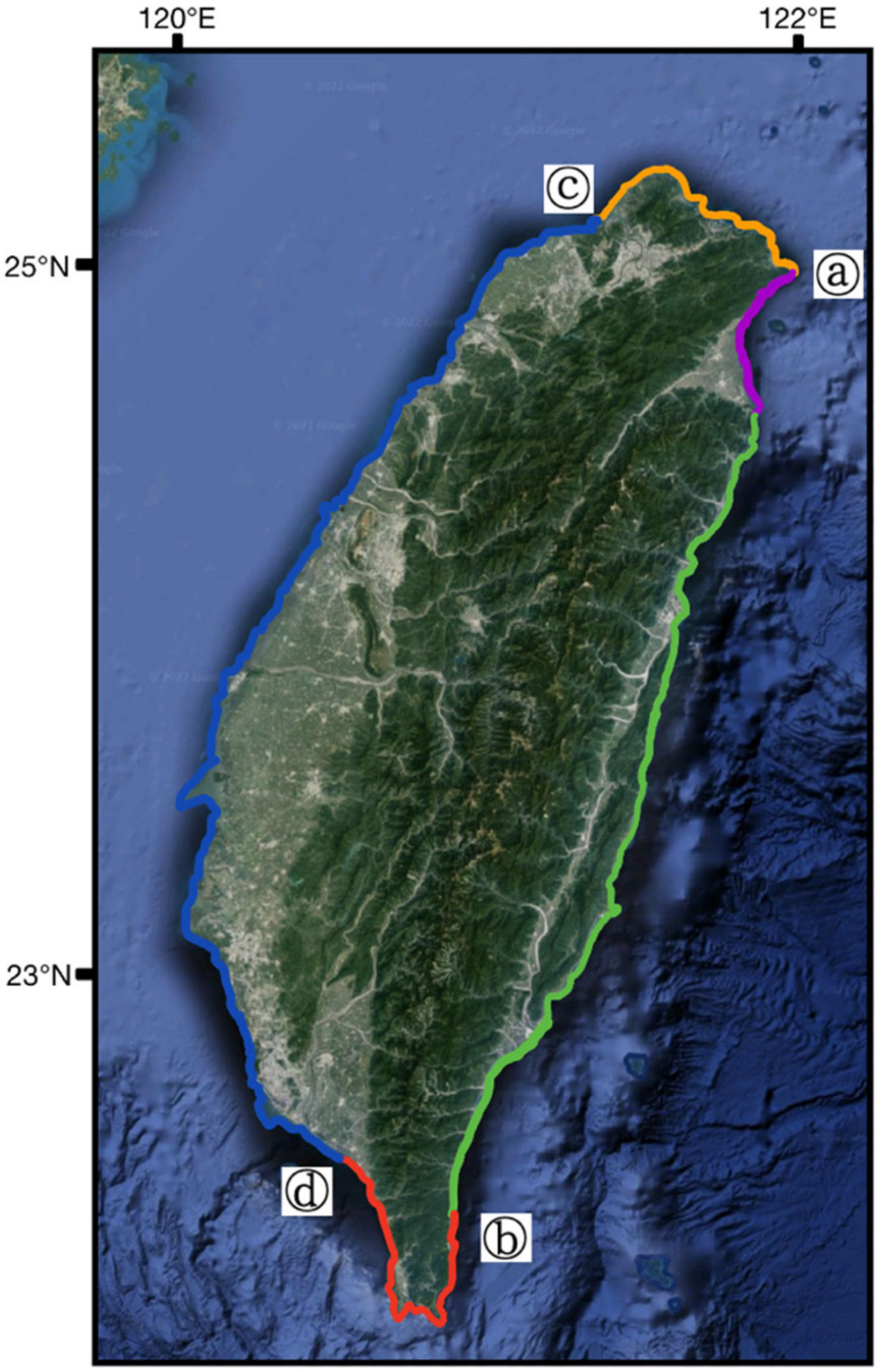
In the study, the shoreline detection was conducted in the coastal area of the main island of Taiwan, between 120°58’E and 122°06’E and 21°53’N and 26°23’N, as shown in Figure 1. Taiwan is located on the eastern edge of the Eurasian tectonic plate, intersecting with the Philippine Sea Plate. The latter keeps moving westward and sliding under the Eurasian Plate, pushing it up at the rate of about 5 mm per year. As a result, almost one-third of the island is over 1000 m above sea level. The coastline of Taiwan’s main island is about 1200 km long, the coastal area is vast, and the coastal terrain is complex. According to the crustal movement, rock formation, slopes, and contours formed by the rising seabed meeting land, generally, Taiwan’s coastal landforms can be classified into four types.

(1)

Eastern fault coast:

This coastal area starts from Santiao Chiao (ⓐ in Figure 1) in the north and ends at the southern tip of the Hengchun Peninsula (ⓑ in Figure 1). The coastal mountains are parallel to the coastline so the eastern coast is mostly rocky, with few bays or islets. In addition, part of the sandy coast is located in the northeast, as shown in purple in Figure 1.

(2)

Western uplifted coast:

This are begins at the mouth of the Tanshui River (ⓒ in Figure 1) in the north and ends at Fangliao in Pingtung County (ⓓ in Figure 1). Since the coast area closes to a deposit plain, it is a straight sandy coast without deep bays. It is a very typical uplifted sand coast. In addition, this area is densely populated and there are many man-made structures, industrial areas, and sandbars near the coastal area.

(3)

Northern mixed coast:

Thid coast goes from the mouth of the Tanshui River (ⓒ in Figure 1) to Santiao Chiao (ⓐ in Figure 1). This mixed coast area is both rocky and sandy, formed by uplifting and depression. The topography of the coast is determined by the rock structure and its resistance to erosion and weathering. Thus, in this area, bays are formed where weak rocks are eroded; capes and headlands are formed where rocks resist erosion and weathering.

(4)

Southern coral reef coast:

This area starts from Fangliao (ⓓ in Figure 1) in the west and reaches to the Hengchun Peninsula (ⓑ in Figure 1) in the east. The reefs appear along this coastline. It is similar to the western uplifted coast, straight, and with few bays. The development of coral reefs is clear evidence of the uplifting process which produced this coastline.

2.2. Ground Data

To evaluate the shoreline detection efficiency, the experimental results of the proposed method were compared with the ground truth data provided by the Construction and Planning Agency Ministry of the Interior (CPAMI). The ground truth data provided by the CPAMI is identified through aerial photos and satellites (including SPOT-6/SPOT-7, IKONOS, QuickBird and FormoSat-5). These government institutions regularly collect aerial photos and high-resolution satellite images of the relatively high tide twice a year. These aerial photos and satellite data are applied in distinguishing and mapping the ground truth data of the shoreline. Furthermore, the draftsmen also actually survey the shorelines on board, especially for the complex man-made development areas. Therefore, the experimental results below will be compared with this manually delineated shoreline ground truth data.

2.3. Sentinel-1 Data

The shoreline detection study was based on the SAR data acquired by the Sentinel-1, an earth observation satellite for the Copernicus Initiative of the European Space Agency (ESA). Sentinel-1 is a constellation of two-satellite, Sentinel-1A and Sentinel-1B, which were successfully launched in 2014 and 2016, respectively, and provide routine acquisitions of global SAR data. Since the revisit period is stabilized at 12 days, two satellites can complement each other so that the revisit time can be 6 days or even less. Thus, Sentinel-1 can offer long-term and large-scale land cover SAR data for the global environment and security monitoring.

In the study area of Taiwan, Sentinel-1 provides VV and VH polarization data with SAR sensors operating in the C-band (central frequency 5.404 GHz). In this study, the Sentinel-1 data was acquired in the interferometric wide swath (IW) mode with a spatial resolution of $5\mathrm{m}\times 20\mathrm{m}$ in range and azimuth, a 250 km swath width, and a level-1 ground range detected (GRD) format with a pixel spacing of $10\mathrm{m}\times 10\mathrm{m}$, ascending and descending orbit modes. The incidence angles of the ascending and descending orbital modes in the study area are from 31.5° to 36.3° and 31.8° to 36.5°, respectively. To cover the entire coastal area of Taiwan, the study collected at least two frames per year from 2016 to 2019, as shown in

Table 1. The acquisition dates of Sentinel-1A data.

	Orbit Mode	Ascending	Descending
Date
2016		01/09, 03/09	06/27
2017		01/27, 03/28	06/10, 08/09, 10/20
2018		02/15	06/29, 12/02
2019		01/05	01/15, 06/12, 09/04

. In addition, the study selected Sentinel-1 images at high tide levels according to the tidal data from the Central Weather Bureau. These Sentinel-1 data are open access and free from the website https://search.asf.alaska.edu/#/ (accessed on 1 July 2021). Therefore, to evaluate the effectiveness of the proposed shoreline detection method, this study constructed a Taiwan shoreline dataset consisting of different types of coastal landforms.

2.4. Sentinel-1 SAR Data Preprocessing

The preprocessing of the Sentinel-1 IW GRD data was accomplished by using the Sentinel Application Platform (SNAP) Sentinel-1 Toolbox software developed by the ESA. First, the radiometric calibration was performed to convert the backscatter intensity to the actual sigma naught ${\sigma }^{°}$ backscatter coefficient in decibels (dB). Thus, the pixel values represent the radar backscatter of the scene in the imagery. Next, range Doppler terrain corrections were applied to remove the geometric distortion in the range due to topography. Then, the range was projected to the Taiwan Datum 1997 (TWD97) earth ellipsoid model. Finally, the speckle noise on the Sentinel-1 data was removed using the Refined Lee Filter [30].

2.5. Training Labels

In the study, the shoreline detection was developed based on the deep learning semantic segmentation network. It is necessary to provide ground truth labels in training machine learning models. Since CPAMI only provides one artificially delineated ground truth data of the Taiwan coastline every year, the ground data is not enough for our research, especially for the detection of current coastline changes. Additionally, there are some discrepancies between the ground truth data and the shoreline shown in the SAR imagery. For example, the difference between the predicted shoreline and ground data for the west coast of Taiwan is large because of the many human developments in the area. This shows the subjectivity of the ground data for manually delineated coastlines. These results will be shown in the following experiments. To alleviate the difficulty of obtaining ground truth data, the study had to create the labels for each radar image, which is a challenging task and requires SAR expertise.

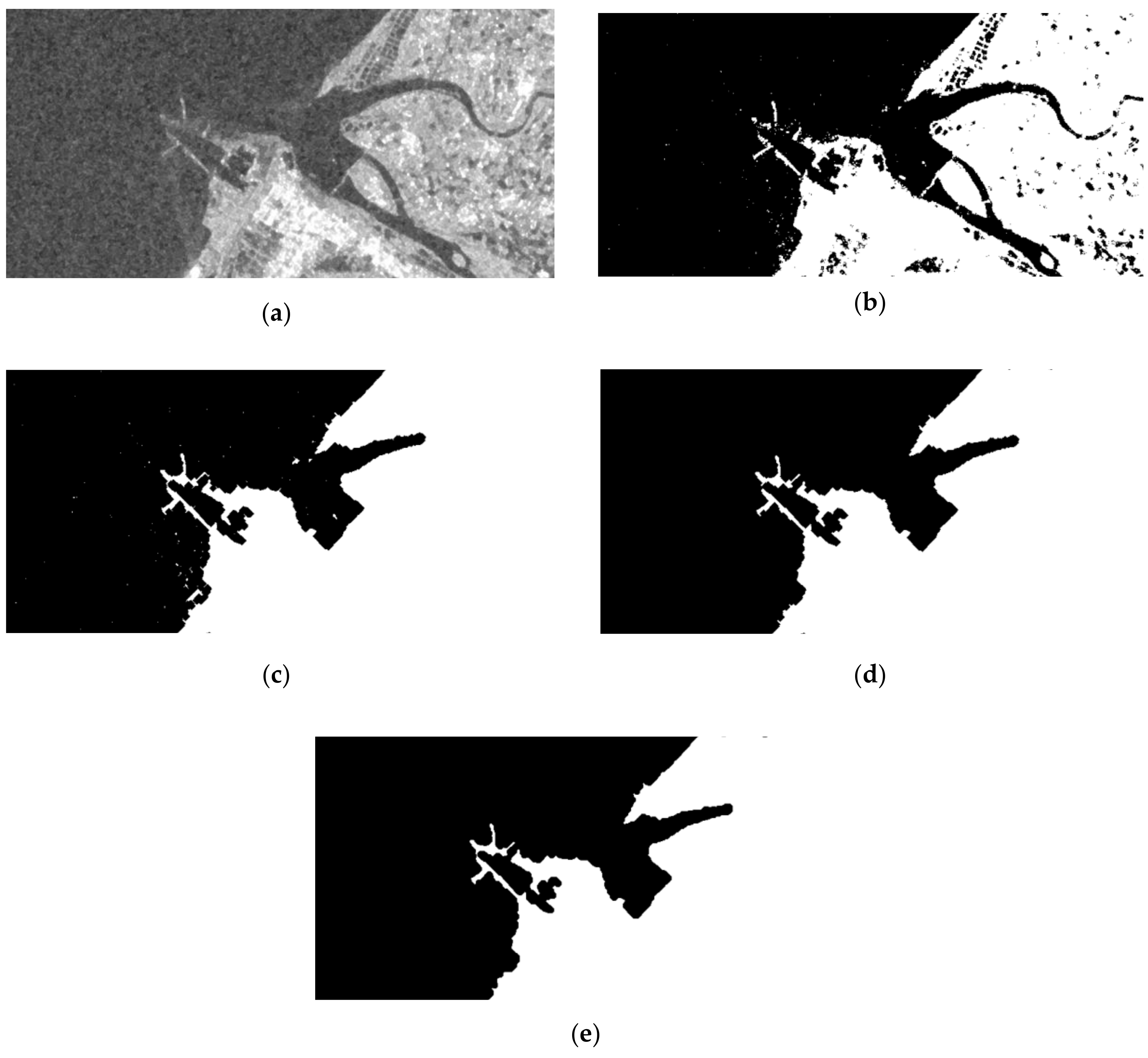
The study performed image segmentation and divided the image into two regions, ocean and land, by using the morphology processing. These results were used to label the Sentinle-1 image, which was the annotation set for the subsequent deep learning network training data. The label processing is shown in Figure 2. First, the study removes small texture details in Sentinel-1 images by opening and closing operations of grayscale morphological processing. Then, the image was binarized by the threshold determined by Otsu’s method, as shown in Figure 2b. Since the average gray level of backscattering from the land is higher than that of the ocean, the land and ocean areas of the image were corresponding to the white and black regions in Figure 2b, respectively. However, there are some fragments in the segmentation results, which come from small textures of the terrain, such as lakes on the land or islands in the ocean. To remove the small textures on the land, the small black objects in the white region were processed by the morphological hole filling operation, so the land area corresponded to the completely white region, shown in Figure 2c. Similarly, to take away the small textures in the ocean, the results of Figure 2c was first converted by negative transformation, so that the ocean corresponded to the white region and the hole filling operation was performed in the region. The result was then converted back by negative transformation, so the ocean corresponded to the complete black region. Therefore, the sea and land were separated into two complete regions, as shown in Figure 2d. Finally, the results were further processed through a morphological closing operation, to smooth the boundary between the land and ocean, as shown in Figure 2e.

The image annotation was done by the described morphological algorithm and assisted by human inspection. The annotated image would be used as an input to train the deep learning model.

2.6. U-Net Model

U-Net is a popular CNN network originally proposed for biomedical image segmentation and has been used in many SAR applications [20]. Considering that U-net can produce more accurate segmentation results with fewer training images, the study utilized U-Net to perform a pixel-level land and sea segmentation.

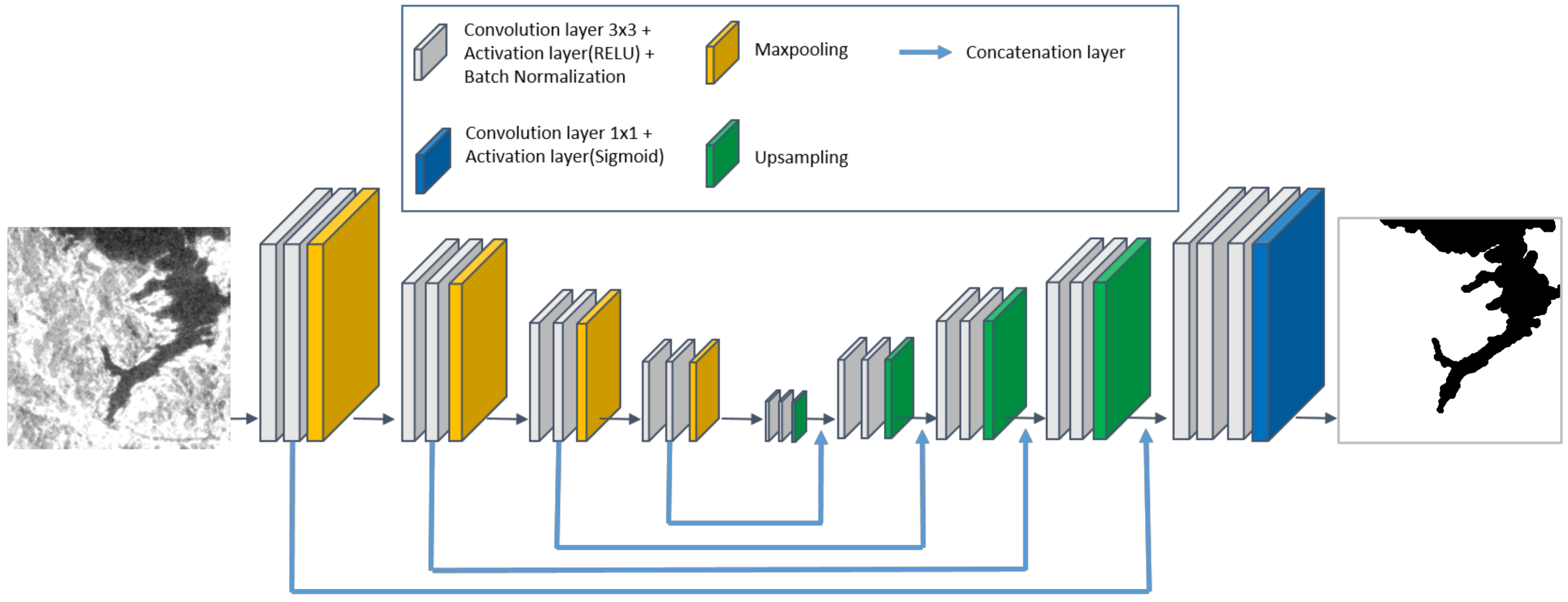
The U-Net architecture, shown in Figure 3, is composed of two parts, an encoder (contracting path) and a decoder (expansive path). The structure of the encoder is similar to a typical CNN. Each encoder block consists of two 3 × 3 convolutional layers, followed by a Rectified Linear Unit (ReLU) used as the activation function in the deep learning model, and a maximum pooling layer with a 2 × 2 kernel and a stride of 2. The decoder contains upsampling, concatenate layers, and two 3 × 3 convolutional layers. The encoder gradually reduces the tensors it receives while increasing the number of features it contains, to capture the meaningful content of the image in a dense vector of features. At the end of each encoder block, the number of feature channels is doubled to learn the complex low-level features. Whereas the encoder gradually compresses the tensor, the decoder gradually enlarges the tensor back to its original size, mapping the meaningful features to their respective locations. In each decoding block, the received tensor is doubled in size by an upsampling process. For the last step, a 1 × 1 convolution is applied to the output of the decoder in order to map the feature vector of each pixel to the desired number of classes, producing a pixel-wise segmentation mask. The pixel value of each map represents the probability that the pixel belongs to the corresponding class.

Additionally, the study added a layer of batch normalization (BN) to U-Net to speed up the network training process and provide the networks stability. The input to each convolutional layer was normalized to a near 0 mean and 1 standard deviation. It can reduce the sensitivity to data variations across layers by normalizing a mini batch of data for each channel. Therefore, BN is playing an essential role in training deep neural networks.

2.7. Post-Processing

After the land and ocean in the SAR image have been detected by U-Net, post-processing the edge, detection is required for the subsequent shoreline extraction. In this study, the Canny edge detection algorithm [31] was utilized to obtain the boundary between the ocean and land, thereby extracting the shoreline.

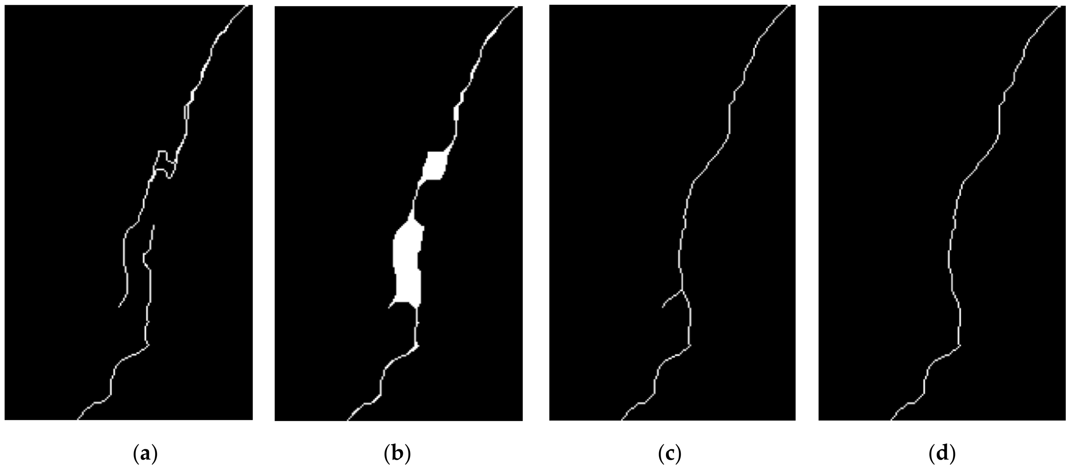
Due to hardware limitations, the acquired SAR images were divided into several sub-images of a small size, such as 256 × 256, for the training of the deep learning network. To avoid some performance degradation in the classification, the sub-images were segmented with a partial pixel overlap. For example, 50 overlapping pixels were used in the experiments below. After the U-Net classification and Canny edge detection, the extracted shorelines of the sub-images must be re-overlapped and merged back to the original image size. Since there may be some differences in the texture and background of each sub-image, the classification results and the detected shorelines are not consistent or fully connected in the overlapping area of the two sub-images, as shown in Figure 4a. The study used morphological processing to address the problems caused by overlapping shorelines. First, the closing and hole filling operations were applied to connect the gaps and fill the holes of the two shorelines. The connected result in Figure 4b showed the thickening of the shoreline. Next, the study used the morphological thinning operation to iteratively remove the boundary of this object while maintaining the connectivity of the shorelines. However, there are some branches in the thinning result of Figure 4c. Then, the morphological spurring operation was used to remove the branches and the final detection result of the shoreline is given in Figure 4d.

3. Results

In this section, the study has conducted a series of experiments on the self-built Taiwan shoreline dataset and evaluated the shoreline detection performance of the different types of coastal landforms to verify the efficiency of our approach. All experiments were performed on a PC equipped with Intel Core i7-8700k with 16 GB of memory, NVIDIA RTX3080 with 10 GB memory, and using CUDA 11.0 with cuDNN 8.0.4. The operating system was 64-bit Windows 10. The study adopted and modified the open-source U-Net [32] framework to train the deep learning models.

The study has collected the Sentinel-1 images of the Taiwan coastal area from 2016 to 2019, as well as the ground truth data provided by CPAMI each year. After the preprocessing by SNAP, the Sentinel-1 images were split into several sub-images of the size 256 × 256 with an overlap of 50 pixels. The Taiwan shoreline dataset constructed in this study contained a total of 4029 images, of which 2021 and 2008 were from the eastern and western coastal areas of Taiwan, respectively. These images were then labeled by morphological processing to create the annotation set. Generally, there are four types of coastal landforms in the dataset, which are mainly divided into the fault coast (rocky coast) in the east, the sandy coast in the west, the coral reef coast in the south, and the headland bay (rocky coast) in the north.

In the study, the shoreline dataset was divided into 70% training images, 20% verification images, and 10% testing images. During training, the number of epochs and batch size were set to 100 and 16, respectively. In addition, the Adam optimizer [33] method was chosen to train the network model. The learning rate was 0.0001 and an early stopping was set by monitoring the value of the validation loss function. 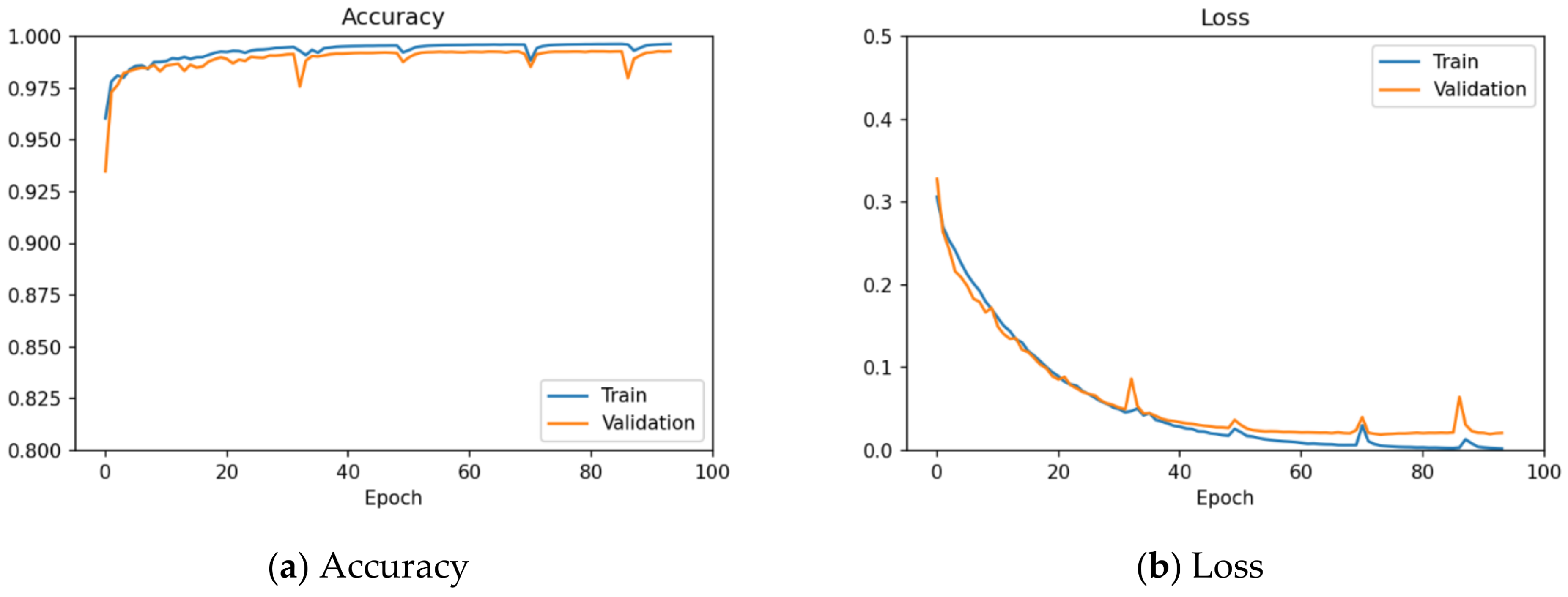Figure 5 showed the training process of the U-Net model. From the training curves, it can be observed that the accuracy has reached 99.5%, with a loss of 0.005. The accuracy and loss of validation set achieved 99.2% and 0.019, respectively.

In the following experiments, to evaluate the shoreline detection performance of the proposed approach, six regions with different types of coastal landforms have been selected. The information for the selected regions is given in Figure 6 and

Table 2. Information of the selected regions.

Region	Located	Landform	Image Size
1	South	Coral reef	734 × 821
2	West	Sandy	256 × 256
3	East	Rocky	783 × 674
4	Northeast	Sandy	727 × 681
5	North	Rocky	1527 × 1603
6	Southeast	Rocky	376 × 473

.

In the study, the F1-measure [34] index was used to evaluate the shoreline detection accuracy, which is defined as:

$$F1-measure=2\times \frac{\mathrm{EP}\times \mathrm{ER}}{\mathrm{EP}+\mathrm{ER}}.$$

(1)

In (1), the edge precision (EP) and edge recall (ER) are defined as:

$$Edge precision\left(EP\right)=\frac{\mathrm{TP}}{\mathrm{TP}+\mathrm{FP}}$$

(2)

$$Edge recall\left(ER\right)=\frac{\mathrm{TP}}{\mathrm{TP}+\mathrm{FN}}$$

(3)

The edge point in the detection results is regarded as correct if the distance between the edge point and the closest ground truth edge point is smaller than N pixels. The ground truth point is considered as being on the edge of the detection results if it falls within N pixels of it. TP and FP represent the number of correct and false edge points on the detection results within N pixels, respectively. FN is the number of undetected edge points on the true ground edge points within N pixels.

3.1. Robust Analysis

The robustness of the proposed shoreline detection method to different types of coastal landforms was verified by the experiments. The experiment evaluated the shoreline detection performance of Region 1~Region 5, selected from Figure 6. Based on the ground truth data, the coastlines of these five regions did not change from 2016 to 2019. Therefore, Sentinel-1 images acquired at different times for these five regions can be regarded as random samples to test the robustness of the shoreline detection model.

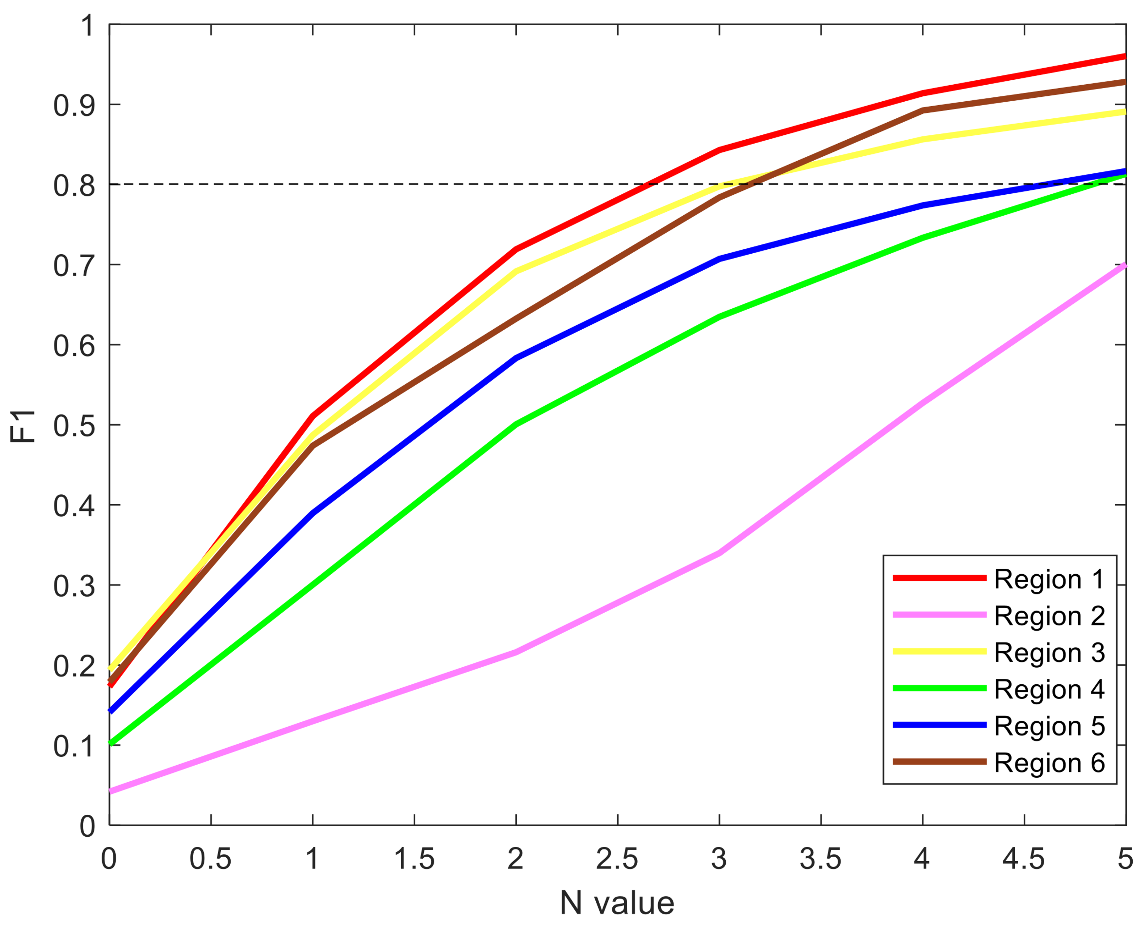
The detection results of the same region at different times/years were compared with each other, and then all the comparison results evaluated by the F1-measure were averaged. The averaged F1-measure for the different regions within N pixels are shown in Figure 7 and

Table 3. F1-measure of five regions by comparing the detection results of proposed method for different samples.

Region	N = 0	N = 1	N = 2	N = 3	N = 4	N = 5
1	0.2001	0.5153	0.7151	0.8438	0.9133	0.9619
2	0.3235	0.6762	0.8355	0.9215	0.9565	0.9724
3	0.2579	0.6286	0.8148	0.8751	0.9144	0.9304
4	0.2099	0.5504	0.7382	0.8464	0.9059	0.9413
5	0.2557	0.5859	0.7551	0.8422	0.8921	0.9204

, where N was set from 0 to 5. The results showed that the performance in Regions 2 and 3 was better, while the performance in Regions 1, 4, and 5 was slightly worse. It can be observed that Region 2 and Region 3 can achieve an over 0.8 F1-measure with N = 2, which means that more than 80% of shoreline edge points detected in different sampled images were within a 2 pixel difference. The N value for Regions 1, 4, and 5 was equal to 3 to achieve an F1-measure in excess of 0.8. Furthermore, when N = 4, approximately a 0.9 F1-measure can be achieved for all five regions. This indicates that there is no significant difference in the detected shorelines within 4 years for these five regions. The experimental results validated the robustness of the proposed shoreline detection method in different types of coastal landforms.

3.2. Shoreline Detection Performance

The experiment evaluated the shoreline detection performance of the proposed approach for different types of coastal landforms through all the selected regions in Figure 6. In addition, the study compared the detection performance of the U-Net model with and without a BN layer and other shoreline detection methods, including the improved fuzzy C-means (IFCM) [27] and statistical model of sea (SMS) [28]. In the experiment, the shoreline detection results of all images acquired from the same selected region in 2016–2019 were compared with the manually delineated ground truth data. As the description of Section 3.1, the comparison results assessed by the F1-measure were then averaged and utilized to evaluate the shoreline detection performance. These averaged F1-measures within N pixels are shown in

Table 4. F1-measure of six regions by comparing the proposed U-Net model and other methods with the ground truth data.

Region	IFCM			SMS			U-Net			U-Net with BN
	N = 3	N = 4	N = 5	N = 3	N = 4	N = 5	N = 3	N = 4	N = 5	N = 3	N = 4	N = 5
1	0.7551	0.8709	0.8973	0.7479	0.8702	0.9321	0.7972	0.8943	0.9544	0.8431	0.9140	0.9603
2	0.3693	0.4281	0.5157	0.3483	0.4692	0.6637	0.3135	0.4884	0.6798	0.3401	0.5273	0.7012
3	0.3128	0.3605	0.4337	0.3863	0.4338	0.5039	0.6212	0.6849	0.7518	0.7977	0.8564	0.8911
4	0.6345	0.7053	0.7632	0.6091	0.7185	0.7879	0.5492	0.6515	0.7477	0.6348	0.7335	0.8133
5	0.6091	0.6890	0.7537	0.6551	0.7263	0.7680	0.6591	0.7199	0.7586	0.7071	0.7739	0.8168
6	0.4524	0.5104	0.5527	0.5216	0.6185	0.7156	0.6676	0.8453	0.8453	0.7839	0.8925	0.9282
Average	0.5222	0.5940	0.6527	0.5447	0.6394	0.7399	0.6013	0.7141	0.7896	0.6845	0.7829	0.8518

and Figure 8.

From the detection results in Table 4, it can be observed that the average F1-measure reached 0.79 and 0.74 at N = 5, for the U-Net without BN layers and SMS, respectively. However, IFCM and poor detection results had a 0.65 average F1-measure at N = 5. The proposed method achieved the highest detection performance, with an average F1-measure of 0.85 at N = 5, which was 0.062 higher than the original U-Net model.

Based on the detection results of all regions of the proposed method, it can be observed that Region 1 performed the best, followed by Regions 3 and 6, then Regions 4 and 5, and Region 2 the worst. Table 4 shows that the F1-measure reached about 0.8 with N values of 3, 4, and 5 for Region 1, Regions 3 and 6, and Regions 4 and 5, respectively. However, Region 2 had poor detection results, with an F1-measure of about 0.7 at N = 5. Regions 1, 3, and 6 are located in the eastern part of Taiwan, with rocky and coral reef landforms, and these coastal areas are less artificially developed. Therefore, the shoreline detection results are closer to the ground truth data. Region 4 is the sandy coasts and Region 5 is the rocky coast, located in the northeastern and northern parts of Taiwan, respectively. Although the landforms of these two regions are different, there are some small ports along the coast. Some man-made developments make it difficult to detect the shoreline. Therefore, the shoreline detection performance of these two regions is worse than Regions 1, 3, and 6. However, the detection performance of Region 2 was worse than other regions, reaching about a 0.7 F1-measure at N = 5. Region 2 is the sandy coast, located in the southwest of Taiwan. Although the experimental results from Section 3.1 showed that there was no significant difference in shoreline detection for different samples in this region. There are many man-made beaches and wave breakers placed along the coast in the region. The proposed method detected the outer contours of man-made developments and regards them as shorelines, but these were not considered coastlines in the ground truth data. Human subjective perception results in a seemingly poor detection performance in Region 2. Thus, if human subjective factors were excluded, the shoreline detection results were close to the ground truth data and the F1-measure of different types of coastal landforms achieved over 0.8 with N = 5.

3.3. Shoreline Change

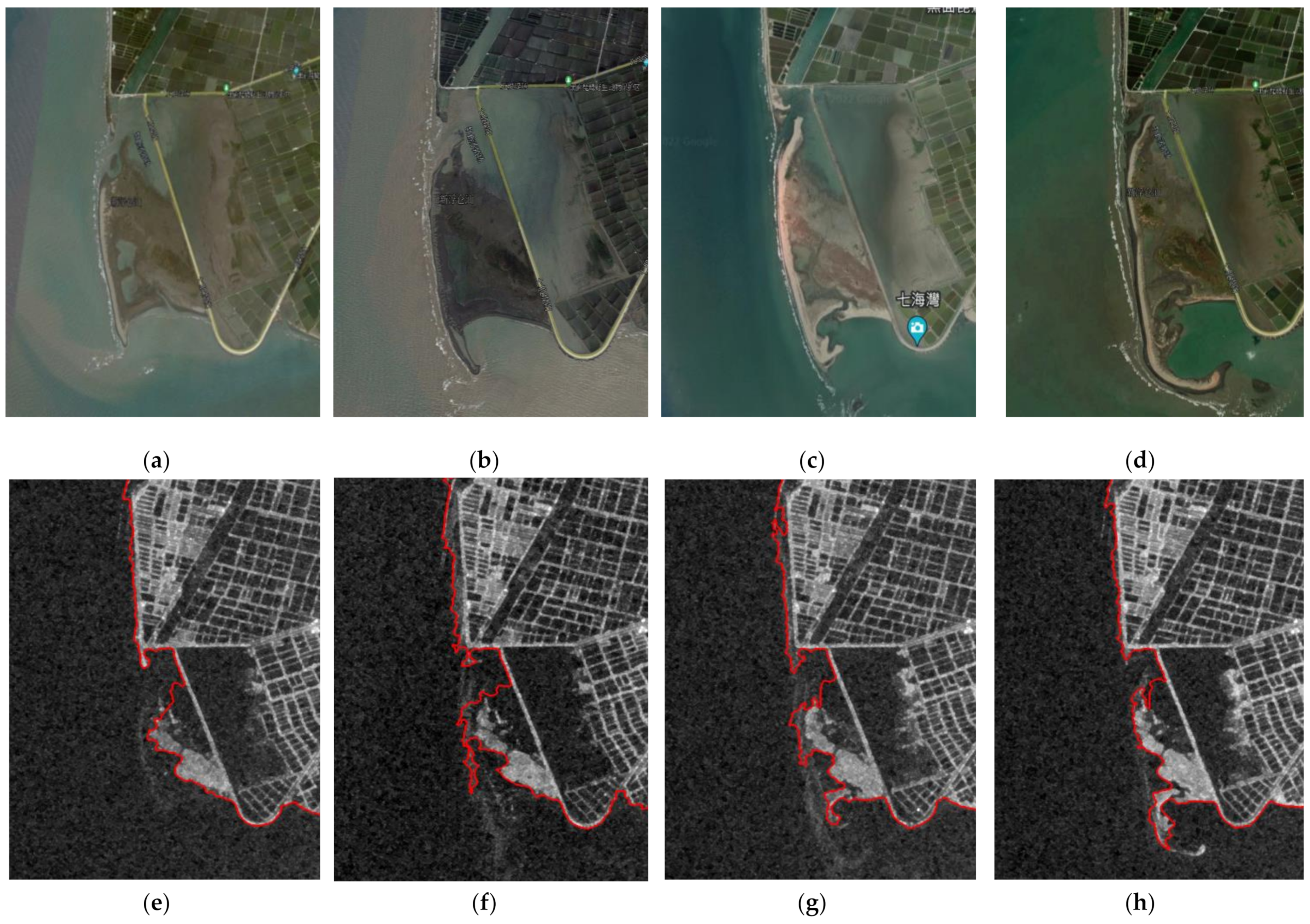
To examine the potential of the proposed method in detecting shoreline changes, the sandbar coastal landform was chosen as the study area in this experiment. The selected region, Xinfu Lunshan, is located in the southwest of Taiwan, which can be described as the extreme western point of Taiwan, and is close to the estuary of the Zengwen River, the longest river in Taiwan. The shoreline of the region has changed significantly over the years due to the river sediment accumulation and coastal currents. The multi-year Sentinel-1 images and the corresponding optical photographs collected from 2016 to 2021 are shown in Figure 9. In Figure 9e–h, the detected shoreline results were represented as red borders and overlaid on the SAR images. From the results in Figure 9, it can be observed that the trend of the shoreline change detected by the proposed method was close to that of the optical photos. 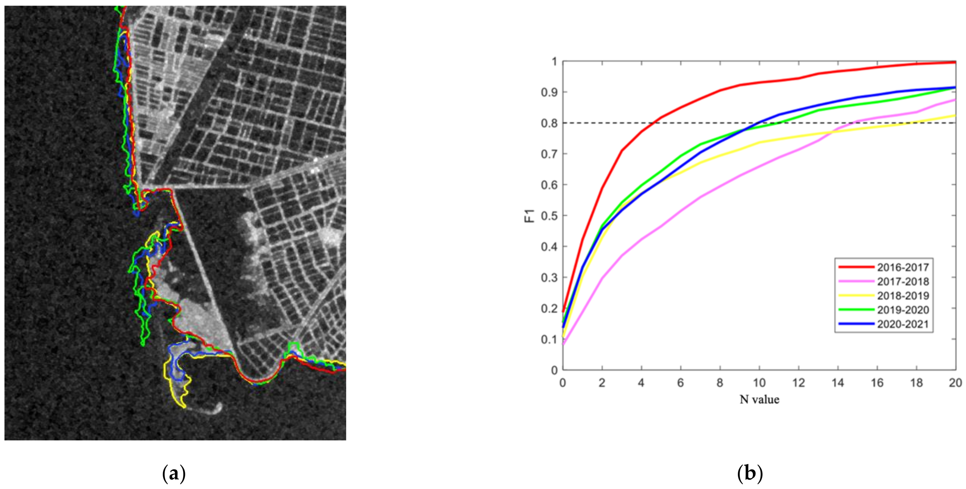Figure 10 showed the shoreline detection results from 2016 to 2021 with different colors. From 2016 (in red) to 2018 (in blue), the Xinfu Lunshan began to expand outward and the sand bar on the south side extended downward. However, the sand bar began to recede inward, but the south side of the sand bar continued to extend downward from 2018 to 2021. In addition, the experiment also compared the shoreline detection results of two consecutive years, as shown in Figure 10. It can be observed that the change from 2016 to 2017 was the smallest, with the F1-measure achieving 0.8 when N = 4. Additionally, the sand bar changed the most between 2017 and 2019, with an F1-measure of about 0.8 at N > 14. The shoreline change was also obvious from 2019 to 2021, with a 0.8 F1-measure when N = 10. The changes of Xinfu Lunshan are not only affected by natural factors, but also by human activities. The sandbar continues to expand westward as the river carries a lot of sediment. After the construction of the Zengwen Reservoir, the sediment was trapped and the expansion of the sand bar was slow. Moreover, the drift direction of the sand land in this area is from southeast to northwest along the coast, which was affected by the coastal currents. Thus, the expansion on the south side of the sand bar forms a hook shape. In addition, there are windbreak forests and dikes on the north side of Xinfu Lunshan. Man-made structures form sediment barriers according to the direction of coastal currents, which can slow coastal erosion. In conclusion, the factors affecting the continuous change of Xinfu Lunshan include the amount of sediment transported by rivers, the direction of coastal currents, and man-made developments. The experiment validated that the proposed method can detect shoreline changes efficiently.

4. Discussion

In this section, the efficiency of the proposed approach for shoreline detection in the entire coastal area of Taiwan was discussed, and the detection performance was analyzed for different coastal areas.

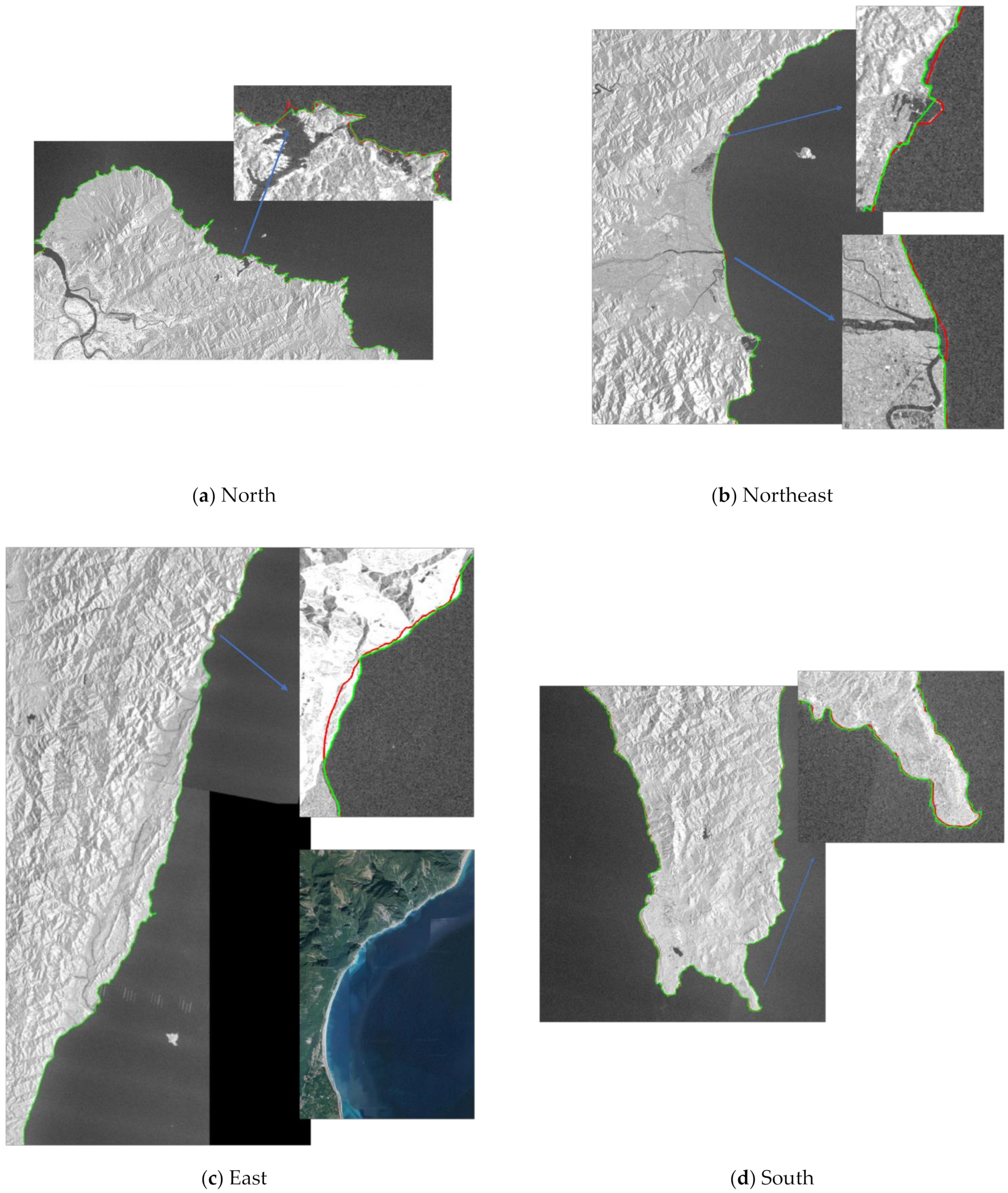
In the experiment, two descending Sentinel-1 VH images from 2019, which cover the entire island of Taiwan, were used. The detected shoreline was divided into six parts: north, northeast, east, south, southwest, and northwest according to the coastal landforms. Each detected result is shown in a different color in Figure 11. 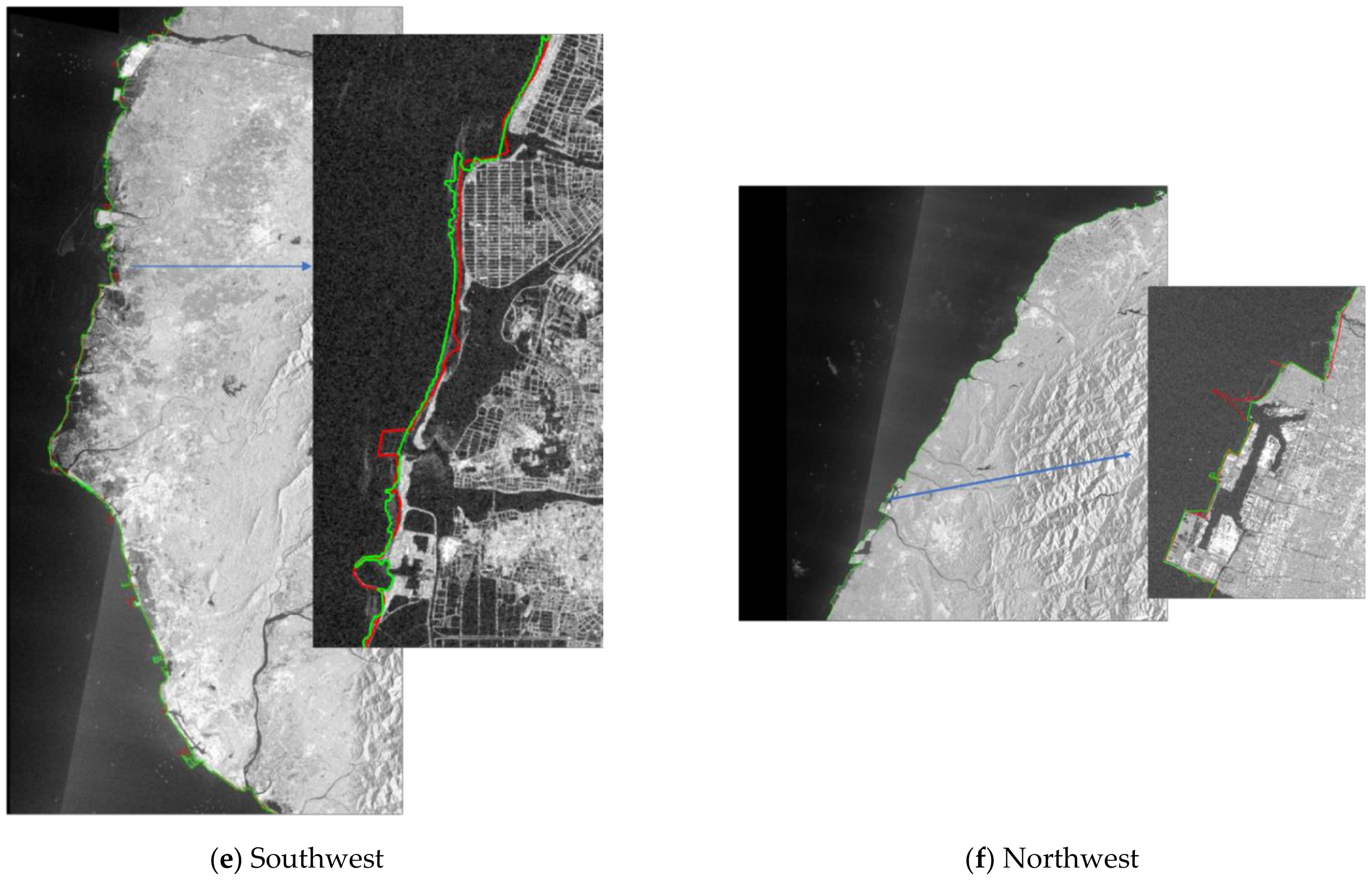Moreover, the detected shorelines were compared with the ground truth data, as shown in Figure 12, where a small image was placed aside to represent the significantly different parts of the comparison.

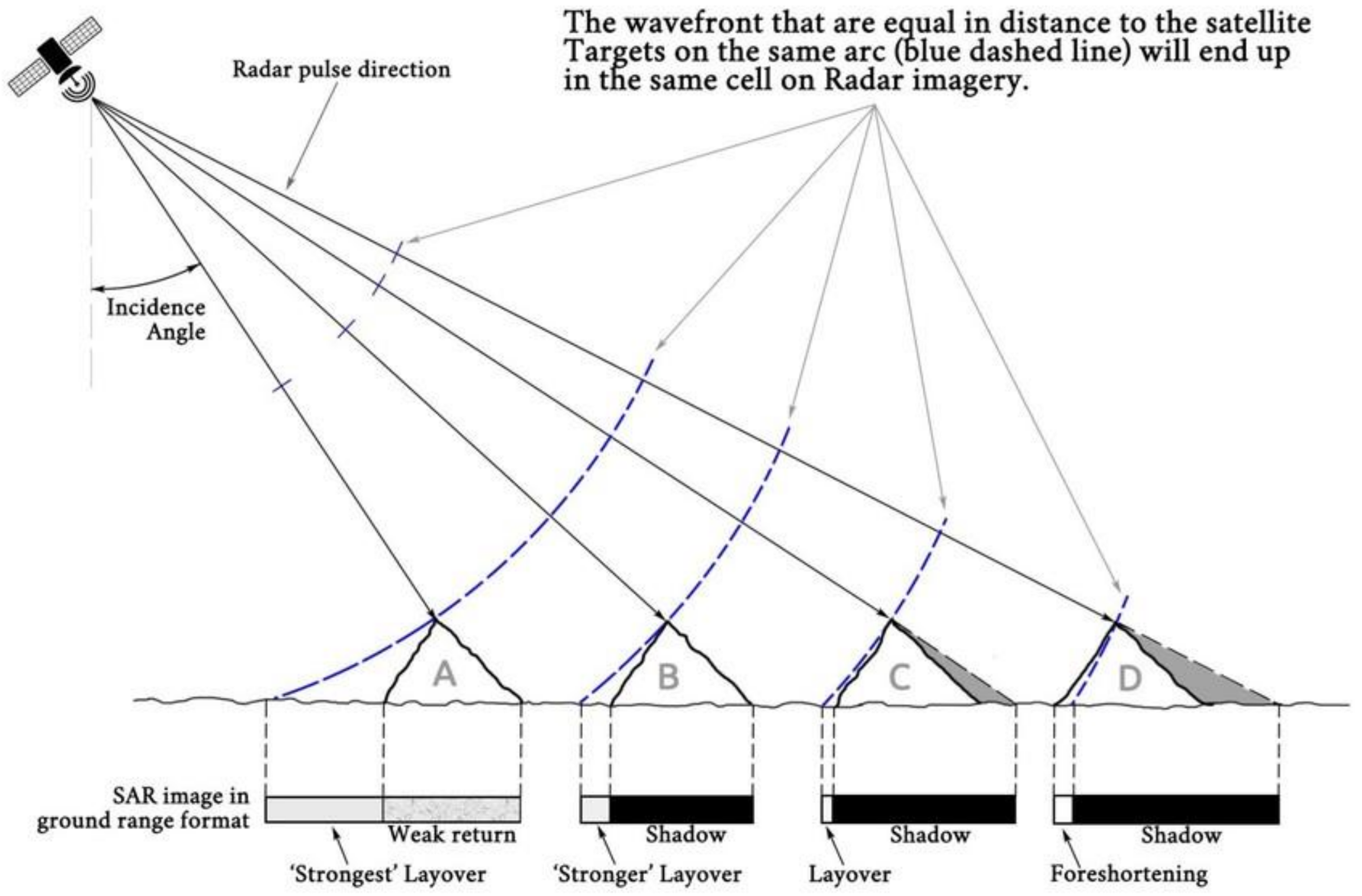
The northern coast of Taiwan is the headland bay (rocky coast) with some ports. In Figure 12a, except for some port areas, the shoreline detection results were close to the ground truth data. The northeast is a straight sandy coast. Apart from some differences in port and estuary locations, the detections were also close to the ground truth data. In the east, there are many continuous mountains that run parallel to the coast. This area belongs to the fault coast. Since the Sentinel-1 descending mode is side-looking from east to west, some regions are affected by the geometric distortion, as shown in Figure 13. This distortion can be observed in Figure 12c by comparing the SAR image with the corresponding optical image. Therefore, some parts of the eastern coast were affected by the physical characteristic of the SAR, resulting in discrepancies between detection results and ground truth data. In southern Taiwan, coral reefs are distributed along the coastal area, causing the detected shoreline to appear tortuous. However, the delineated ground truth data appeared smoother, so there were subtle differences compared to the detection results, as shown in Figure 12d. The western coast of Taiwan is sandy. In the analysis below, this area was divided into southwest and northwest parts according to the degree of coastline change. The coastline of the southwest region varies greatly, for example, Xinfu Lunshan shown in Figure 9 is located in this region. There are many man-made developments on the coast, such as harbors, dikes, and industrial areas. In addition, the deposition and erosion on sandbars are also natural factors for shoreline changes. In the area, the large ports and the accumulation of sediment in the estuary have resulted in the detected shoreline to appear tortuous. As displayed in Figure 12e, the ground truth data was depicted more smoothly, which resulted in larger discrepancies with the detection results. Finally, in the northwest area, the shoreline changes less in the region than in the Southwest. As shown in Figure 12f, the dikes of the harbor cannot be detected completely due to the resolution of the Sentinel-1 data. Except for these man-made structures, the detected shorelines in this area closely matched the ground truth data.

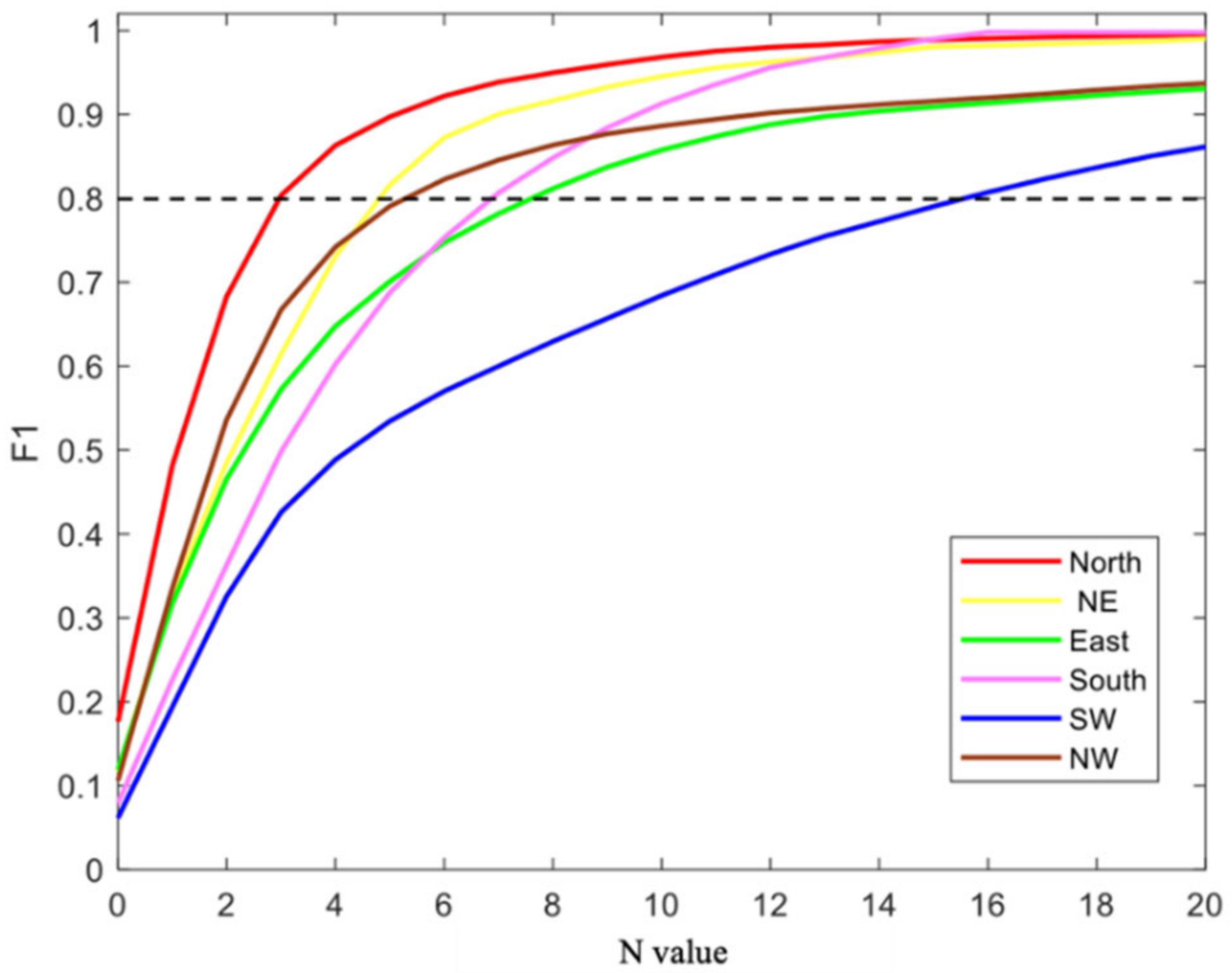
Next, the detected shoreline was compared with the ground truth data and the detection performance of the six regions was evaluated by F1-measure. From Figure 14 and

Table 5. Performance evaluation of shoreline detection in different regions.

Location	N (F1 > 0.8)	Length (Pred.) (Pixels)	Length (GT.) (Pixels)	Pred. Length Error (%)	Landform
North	3	12,273	12,213	0.49%	Headland bays
Northeast	5	7704	7737	0.43%	Sandy
East	8	30,522	32,690	6.63%	Rocky
South	7	16,166	15,309	5.60%	Coral reef
Southwest	15	29,966	27,799	7.80%	Sandy
Northwest	4	23,737	25,136	5.57%	Sandy

, it can be observed that the proposed approach had the better detection performance in the north, northeast, and northwest regions, with the F1-measure above 0.8 when the N value was 3, 5, and 5, respectively. Then, the detection performance in the eastern and southern regions ranked the second, with the F1-measure reaching over 0.8 at N = 7 and N = 8, respectively. Due to the geometric distortion of the SAR data in the eastern region and the smoother delineation of the ground truth data in the southern region, the shoreline detection results in these two regions were slightly worse. Finally, the proposed method was less effective in the southwest region where the sandbars changed greatly and lots of artificial structures were built. In this region, the F1-measrue achieved about 0.8 with N = 15. In addition, the shoreline length prediction errors were evaluated, as shown in Table 5. The smallest length prediction error was in the northern and northeastern regions, which were 0.49% and 0.39%, respectively. In the southwest region, the error was the largest, reaching 7.80%. The average predicted length error of these regions was 5.53%. The entire shoreline length of the island in Taiwan was 120,884 and 120,368 pixels, respectively, evaluated by ground truth data and detection results. In conclusion, the performance of the proposed method in the shoreline detection of Taiwan was better in the north than in the south, and in the east than in the west.

5. Conclusions

This study proposed a U-Net-based method for Taiwan shoreline detection from SAR images. The performance of the proposed method was validated by experiments on the study area of Taiwan, which has a variety of complex coastal landforms including rocky, sandy, headland bays, and coral reefs. In this research, the U-Net model was trained on a self-built shoreline dataset, which contained Sentinel-1 SAR images collected from 2016 to 2019 in the coastal areas of Taiwan. The shoreline detection result was evaluated by the F1-measure and compared with the related methods. The experimental results showed that the proposed method achieved over 80% of the F1-measure within a 5 pixel difference between the detected shoreline and the ground truth data for different coastal landforms. In addition, it has been verified that the proposed method can detect the changing trend of the shoreline of the Xinfu Lunshan sandbar, where the changes were obvious from 2016 to 2021. Furthermore, the entire shoreline of Taiwan was depicted by using the detection results and these results were analyzed for different coastal landforms. The detected shoreline length of the Taiwan island was 120,368 pixels (10 m/pixel), which was about 1200 km long and close to the actual coastline length of Taiwan. In conclusion, the proposed method achieved a high shoreline detection performance in different coastal areas of Taiwan, especially in describing the shoreline changes. The future work will focus on extending the proposed model to the shoreline detection of other islands.