Abstract
Hyperspectral image classification methods based on deep learning have led to remarkable achievements in recent years. However, these methods with outstanding performance are also accompanied by problems such as excessive dependence on the number of samples, poor model generalization, and time-consuming training. Additionally, the previous patch-level feature extraction methods have some limitations, for instance, non-local information is difficult to model, etc. To solve these problems, this paper proposes an image-level feature extraction method with transfer learning. Firstly, we look at a hyperspectral image with hundreds of contiguous spectral bands from a sequential image perspective. We attempt to extract the global spectral variation information between adjacent spectral bands by using the optical flow estimation method. Secondly, we propose an innovative data adaptation strategy to bridge the gap between hyperspectral and video data, and transfer the optical flow estimation network pre-trained with video data to the hyperspectral feature extraction task for the first time. Thirdly, we utilize the traditional classifier to achieve classification. Simultaneously, a vote strategy combined with features at different scales is proposed to improve the classification accuracy further. Extensive, well-designed experiments on four scenes of public hyperspectral images demonstrate that the proposed method (Spe-TL) can obtain results that are competitive with advanced deep learning methods under various sample conditions, with better time effectiveness to adapt to new target tasks. Moreover, it can produce more detailed classification maps that subtly reflect the authentic distribution of ground objects in the original image.
1. Introduction
Remote sensing (RS) is an irreplaceable means to perceive the earth [1]. As one of the most significant branches of the RS field, hyperspectral imaging technology can capture provide surface spectral information [2]. Therefore, the characteristic of spatial information and spectral information fusion in the hyperspectral image (HSI) makes it possible to identify and classify ground objects accurately. HSI classification is one of the essential topics of hyperspectral signal processing. It can convert hyperspectral images with hundreds of bands into classification maps through pixel-by-pixel category labeling, so as to intuitively reflect the distribution information of ground objects in the images. However, the data characteristics of HSI such as high-dimensional nonlinearity and spectral mixing, etc., bring great challenges to the classification task.
In this paper, to achieve image-level feature extraction, we look at the three-dimension global HSI data which include hundreds of contiguous spectral bands from a sequential image perspective. Thus, the difference between the two arbitrary single sequence images in adjacent spectral bands reflects the global spectral variation information between them. Considering that the optical flow estimation task in computer vision is a crucial method by which to extract the motion information of contiguous frames from video data, we attempt to extract the global spectral variation information between adjacent spectral bands by using the optical flow estimation method.
On the other hand, current deep-learning-based HSI classification methods with outstanding performance usually depend on sufficient training samples because of the large number of trainable parameters in the model. Moreover, the generalization ability of models is poor, and it is time-consuming to retrain the model when facing a new target image. To solve these problems, we utilize the transfer learning strategy, a technique that applies knowledge or patterns learned in one domain to a different but related domain [3].
Therefore, to detect global spectral variation information effectively through accurate optical flow estimation so as to achieve discriminative image-level feature extraction, the PWC-Net [4] was applied in our proposed method. The PWC-Net is a compact, efficient and advanced network for optical flow estimation. We transfer the PWC-Net pre-trained with video data to the feature extraction target task, and an innovative data adaptation strategy is proposed to bridge the gap between the HSI and video data. This allows us to extract image-level features utilizing knowledge learned from the video data by PWC-Net, avoiding the sample dependence and model retraining. Then, we choose the frequently-used support vector machine (SVM) [5] as the classifier for our method. Simultaneously, benefiting from the efficient training and classifying of SVM, we propose a vote strategy combined with image-level features at different scales when classifying so as to further improve the accuracy. On the whole, the main contributions of our work can be summarized as follows:
- 1.
- We propose an image-level feature extraction method to achieve more refined HSI classification, avoiding the inherent defects accompanying the previous patch-level methods.
- 2.
- We look at the global HSI with hundreds of contiguous spectral bands from a sequential image perspective and extract the global spectral variation information between adjacent spectral bands using the optical flow estimation method.
- 3.
- We transfer the optical flow estimation network PWC-Net that is pre-trained with the video into the HSI feature extraction target task. To our knowledge, this is the first work that transfers a network pre-trained on video data to HSI classification with excellent performance.
- 4.
- We design a vote strategy in the classification phase, which utilizes features at different scales to construct multiple tasks and votes for obtaining the optimal results, so as to further improve the classification accuracy.
The sections of the paper are arranged as follows. Section 2 describes related work. Section 3 describes the image-level feature extraction method based on transfer learning (Spe-TL) in detail. Section 4 mainly consists of experimental details, results and analysis. Finally, Section 5 concludes the article comprehensively.
2. Related Works
2.1. Hyperspectral Image Classification
Early traditional HSI classification methods usually divide processing into the following two stages: feature extraction and classification. Among them, spectral feature extraction technology represented by Principal Component Analysis (PCA) [6], etc., spatial feature extraction technology represented by Gabor [7], Extended MorphoLogical Profiles (EMP) [8], Local Binary Pattern (LBP) [9] and classifiers such as Support Vector Machine (SVM) [5] are widely used. However, the traditional methods overly rely on artificial feature design, which makes it difficult to fully extract discriminative features for classification, resulting in a poor classification accuracy and poor model robustness, etc.
The methods based on deep learning have been widely used in HSI classification. Compared with the traditional methods, they can learn more discriminative features adaptively by relying on data. After several years of development, these approaches can be roughly divided into those including spectral features, spatial features, or joint spectral–spatial features according to different feature extraction levels. As approaches that take the whole image as input have been popularized recently, these models can also be divided into different types according to the form of input, such as pixel-level, patch-level, and image-level. The approaches that take the spectral sequence of one pixel as a 1D vector as their input can be called pixel-level approaches, such as stacked autoencoder (SAE) [10] and 1D convolutional neural network (1D-CNN) [11], etc. Then, in order to make use of both spectral and spatial information, the original image is segmented into a series of local patches in the central pixel neighborhood as input, which can be called the patch-level classification approach. For example, the approaches with a 2D convolutional neural network (2D-CNN) [12,13], the approaches with 3D convolutional neural network (3D-CNN) [14,15,16,17,18,19], and other novel models, such as the method based on a capsule neural network [20], transformer [21,22], etc., have been developed. Although patch-level approaches have made significant progress as the mainstream approach, they still have several inherent defects, which are as follows: (1) the distance of information capture is restricted to a limited range of local patches, which leads to the inability to establish long-distance information correlation; (2) the original image must be pre-sliced, which makes a lot of information redundant between patches, increasing the extra computing overhead; (3) the center pixel category is regarded as the category of the whole patch when classifying. However, a simple rough label is insufficient to provide complete spatial distribution information in complex observation scenes.
Therefore, using the global image as input can effectively avoid the flaws of the patch-level method. This alternative method, which can be called the image-level method [23,24,25,26,27,28,29], is gaining popularity. The practice proves that the image-level method can improve classification accuracy and efficiency.
However, we note that current feature extraction methods based on deep learning are all pixel-level and patch-level [30,31,32,33]. Therefore, the successful implementation of the image-level classification method prompts us to attempt to research the special image-level feature extraction method based on deep learning, so as to obtain more powerful discriminative features conducive to classification.
2.2. Transfer Learning
Deep learning based on data-driven methods has achieved significant success in diverse tasks and demonstrates great potential. However, the artificial intelligence (AI) system constructed using the foundation of data-driven methods is vulnerable and poorly generalized. Simultaneously, data and labeled samples are often lacking in terms of realistic task scenarios. To move toward genuine intelligence, transfer learning combines knowledge-driven and data-driven learning, aiming to solve the dilemma of learning with insufficient labeled samples for a target task by transferring knowledge learned from source tasks, so as to develop reliable and extensible AI technologies [34].
The scarcity of training samples is also a general reality in HSI classification tasks. Although classification methods based on deep learning have led to great achievements, these methods with outstanding performance are also accompanied by excessive dependence on the number of samples and complex re-training on the target HSI scene. In recent years, the transfer learning strategy has been introduced to solve these problems. In the early period, Yang et al. attempted to pre-train and transfer the low and middle layers of the network on the source dataset and fine-turn the top layers on the target dataset; however, it should be kept in mind that the source and the target set are just different scenes obtained by the same sensor [30]. Windrim et al. [35] and Zhong et al. [36] further attempt to achieve transfer learning with cross scene and sensors. The above works belonging to homogeneous transfer learning still require an HSI containing a large number of labeled samples as source data. Based on the cross-sensor strategy, Zhang et al. further explored the cross-modal strategy, in which the network is pre-trained on RGB natural image datasets by inflating the 2D natural images to 3D cubes to resolve the issue of dimensionality mismatch and then fine-tuned them with the target HSI [37]. The cross-modal strategy is an example of the heterogeneous transfer learning strategy, and He et al. go one step further by applying the VGGNet pre-trained on an ImageNet dataset to the target task of HSI classification and mapping the HSI to the three-channel data when fine-turning to align heterogeneous data [38]. Heterogeneous transfer learning enables a network to pre-train on a large number of existing heterogeneous natural image datasets, so as to effectively avoid the limitation of the scarcity of labeled samples in HSI, no matter the source or target data.
Our proposed method also belongs to heterogeneous transfer learning and this is the first work that transfers a network pre-trained on video data to an HSI classification target task. Furthermore, the former methods based on transfer learning for HSI classification are all patch-level as far as we know; that is, the HSI must be segmented to patches as input in the pre-training or fine-turning phase. Additionally, the proposed method directly takes the global HSI as input, making a conducive pioneering exploration of image-level methods based on transfer learning for HSI classification.
2.3. Optical Flow Estimation
Optical flow is a significant concept in computer vision (CV). The motion of an object in 3D space is reflected in the video to form the brightness motion of the image, and the visible motion of the brightness mode produces the optical flow. Thus, optical flow is the instantaneous velocity of the motion of pixels on the observed imaging plane of a 3D moving object. Figure 1 shows two random images and their corresponding ground-truth optical flow in MPI-Sintel [39] datasets. Optical flow estimation can express the motion of objects by extracting fine and dense matches, which is widely used in action recognition [40], moving objects segmentation [41], aided driving [42], and other fields.
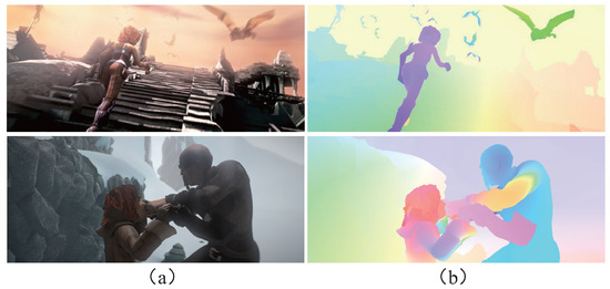
Figure 1.
Optical flow diagram. (a) Image. (b) Ground truth flow.
Horn and Schunck proposed the Horn–Schunck (HS) algorithm [43] in 1981, which is a form of the variational method, and carried out the pioneering work of optical flow estimation. The variational method is a classical and traditional optical flow method, and a numbers of works [44,45,46,47,48] that aim to improve this method based on the HS have promoted its development. The characteristics are that multiple constraints are incorporated into the classical energy minimization framework. Large Displacement Optical Flow (LDOF) [49] initially incorporated the descriptor matching component into the variational method to solve the large displacements situation. Then, a series of improvement methods with rigid matching descriptors [50,51] were developed to help avoid the performance deterioration at small displacement locations. Furthermore, to effectively deal with the fast, non-rigid motion, a non-rigid dense matching algorithm is designed for DeepFlow [52]. Although the continuous optimization of the variational method can achieve good optical flow results, the long computation time caused by high computational complexity limits its wider application.
With the rise of deep learning in computer vision, early works using deep learning to estimate optical flow usually utilize CNN as a high-level feature extractor [53,54]. The extracted matching component of the feature is used to replace the data term in the variational approach, so these works do not represent a learnable task. FlowNet [55] is the first attempt to consider optical flow estimation as a learnable task. FlowNet utilizes CNN to extract the features of adjacent frames and establishes the corresponding correlation of pixels, so as to achieve optical flow estimation. Furthermore, this supervised estimation paradigm has been adopted and refined. FlowNet2.0 [56] deepens the network by stacking multiple layers and introduces a subnetwork aiming for small motions, which effectively enhances the estimation performance. Some subsequent works concentrate on improving the network architecture to obtain more accurate results, such as SPyNet [57], Liteflownet [58], etc. Among them, PWC-Net [4], as a compact and effective network, achieves excellent results in the task of optical flow estimation under the supervised learning paradigm. To this day, it is still widely used in diverse tasks. Thus, we also utilize the PWC-Net as the fundamental model in our research. Additionally, to overcome the limitation caused by the scarcity of true optical flow labeled samples in supervised learning paradigms, some studies [59,60,61] based on self-supervised training allow the network to be trained in the video without labels. This kind of task usually uses the optical flow to reduce the difference between the target image and the reference image to design the specific loss function for the network to learn. Advanced self-supervised learning methods have achieved competitive results with supervised learning methods, and this research area will continue to attract interest in future.
3. Materials and Methods
In this section, we will describe the proposed image-level feature extraction method with transfer learning (Spe-TL) in detail. The illustration for our approach is shown in Figure 2. Firstly, in order to achieve image-level feature extraction, it is necessary to utilize the global image as input; therefore, we used a hyperspectral image with hundreds of contiguous spectral bands from a sequential image perspective. Therefore, the difference of arbitrary two single sequence images in adjacent spectral bands actually reflects the global spectral variation information between them. Then, we extract the global spectral variation information between adjacent spectral bands by using the optical flow estimation method. Secondly, in order to take advantage of the abundant knowledge of the model learned during the optical flow estimation source task, avoid sample scarcity during the target task, reduce the time consumption and bypass the need to re-train the model, etc., we utilize the transfer learning strategy and propose an innovative data adaptation strategy so that the optical flow network pre-trained on video data can be applied to the image-level feature extraction target task. Then, by continuously inferring the global variation information between spectral bands, such information is finally concatenated to obtain the image-level feature; this process of feature extraction does not require any labeled samples. Finally, we utilize the traditional classifier SVM to achieve classification. Benefiting from the efficient training and testing of SVM, we propose a vote strategy. We utilize features at different scales to construct multiple tasks of training and classification and obtain multiple classification results; then, the optimal result is finally obtained by voting. The vote strategy could further improve the classification accuracy. Next, the essential components of our method will be elaborated on in the following four subsections.

Figure 2.
Illustration of the proposed hyperspectral image-level feature extraction based on transfer learning (Spe-TL) for hyperspectral image classification.
3.1. PWC-Net
Since the PWC-Net [4] has been proven to be an efficient and accurate optical flow estimation network for various tasks, we chose the PWC-Net as our basic network. Compared to FlowNet 2.0 that stacks multiple networks leading to complex training and an exponential increase in the number of trainable parameters, the PWC-Net utilizes multi-scale features to replace stacked networks, and it uses warping and cost volume operations that not only enhance the quality of optical flow estimation but also minimize the model size with no learnable parameters. The illustration of the network is shown in Figure 3. The left side in the figure is the illustration of the overall information flow, and the right side is the course-to-fine procedure in PWC-Net. For input images (h and w denote height and width of image, and the RGB images have 3 channels), the -level pyramid features are generated by -1 continuous convolution layers with a downsample factor of 2. The value of L actually determines the number of layers of the pyramid extractor and the depth of the network. Additionally, the setting also requires a consideration of the size of the input because the smaller input cannot be processed in the deeper pyramid extractor. A learnable feature pyramids extractor can learn the conducive representation of multi-scale features with fewer number of trainable parameters. Take the input image as the bottom feature, that is, , so the top feature is . The index t denotes the serial number of two images as input (t = 1,2). At the -th level (1), the operation of the warping layer can be formulated as follows:
where x denotes each pixel in the image and denotes the optical flow estimation results calculated by the former-level pyramid features. The warping operation has been proved to be a critical principle of traditional approaches to estimate large motion [62], which is taken as a pivotal layer with no learnable parameters in the network for the same purpose. Next, the cost volume that represents the matching cost between two frames is constructed by the features of the first image and warped features of the second image :
where N is the length of the column vector and the channel dimension of feature , which varies by layer from 16 to 32, 64, 96, 128 and 196. The and denote each pixel in the first image and the corresponding matching pixels in the second image, respectively. The only needs to be calculated on a limited range of d pixels, that is, . The range of d is actually the size of the searching window, which should be smaller than the size of the feature maps at the l-th level, so the range of d is [1, ]. If the d is too large, it will lead to a huge computational overhead and no performance improvement; too small a d will lead to insufficient matching retrieval. The cost volume is a more discriminative representation of optical flow; therefore, a cost volume layer with no learnable parameters in the network can enhance the final estimation results of optical flow. Then, the results of the cost volume layer , , and after upsampling are used as the input of the optical estimator. The estimator deploying multiple convolution layers with a dense connection decreases the number of feature channels layer by layer, and the whole estimation process is iterative until the bottom level. Finally, the context network is constructed to further refine the optical flow after completing the estimation of the final level. It deploys seven layers with dilated convolution (kernel size is 3 × 3) and the dilation coefficient that controls the spacing between the kernel points gradually increases, which can effectively expand the receptive field so the context information of a larger range can be captured.
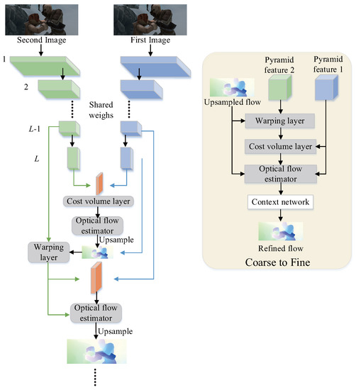
Figure 3.
Illustration of the PWC-Net architecture and its course to fine procedure.
3.2. Training and Transfer Learning Strategy
For source domain , source task , target domain , and target task , the purpose of transfer learning is to acquire knowledge in and to help achieve the in the , as shown in Figure 4. In our method, we aimed to extract the image-level feature by continually capturing the variation information in adjacent spectral bands. So the target task is established, and the target data are represented by hyperspectral images awaiting classification. First, the extraction of an image-level feature requires the global image as the input. Second, we look at the three-dimension global HSI data from a sequential image perspective, so the number of single-band sequence images is C. Thus, the difference between two arbitrary single sequence images and in adjacent spectral bands reflects the global spectral variation information between them, which can be formulated as follows:
where x denotes the same location of the pixels. Such global variation information provides a supplementary image-level feature that effectively enhances the original feature. Third, the motion of the object in 3D space is reflected in the image to form the brightness mode motion of the image, and the visible motion of the brightness mode produces the optical flow [49], which contains a horizontal motion component and a vertical motion component of pixels. Since the HSI is a static scene with no movement in the spatial dimension, we use the optical flow estimation method to calculate the variation information in the spectral dimension, which denotes the direction and degree of variation at the current point of the spectral curve. Capturing the variation information depends on the inference of the transferred optical flow network. The PWC-Net is utilized as source network in the proposed method. Therefore, the PWC-Net is pre-trained on the source data (video data) in the source domain, and a multi-scale loss function [55] is utilized when training, which is as follows:
where denotes the space of trainable parameters, defining the set of all the learnable parameters in the optical flow estimation network, PWC-Net, which includes the feature pyramid extractor and all optical flow estimators. denotes the optical flow estimated by the network at the l-th level, denotes the corresponding labels for supervised learning, denotes the contribution weight of the -th level loss component, and is a trade-off weight for the second term which regularizes the parameters of the model.

Figure 4.
Illustration of transfer learning.
After pre-training is completed, the pre-trained PWC-Net is used as the target network. Then, a common practice is to extend the network according to the requirement of the target task and fine-tune part or all of the network with target data. However, we observe that this practice not only requires target training samples but also has a poor classification effect in the experiment, which indicates that this fine-tuning method for classification tasks weakens the original ability of the network to capture the variation information. On the other hand, a satisfactory classification effect is achieved when the transferred network is directly utilized to capture variation when extracting image-level features, which indicates that the variation in the captured knowledge of a network trained with the source video data can to be transferred to the HSI feature extraction task for better classification. Therefore, we adopt the latter practice.
3.3. Data Adaptation for Feature Extraction
For heterogeneous transfer learning, a pivotal step is bridging the gap between source data and target data. The optical flow network is pre-trained on the video datasets that are actually composed of RGB 3-channel sequence images. Additionally, the input of the source network is two adjacent frames in the video. In order to capture the variation information between adjacent spectral bands and make the hyperspectral image data adaptable for the transferred network, we look at HSI with hundreds of contiguous spectral bands from a sequential image perspective. Then, the following two data adaption strategies are proposed to achieve the target task: (1) Simply copy an arbitrary single-band image and then synthesize a 3-channel image; and (2) arbitrary three consecutive single-band images can be taken as a 3-channel image. We observe that the latter strategy can achieve a better discriminative feature, which denotes three consecutive single-band images as the input can better reflect the spectral variation information. Thus, we utilize the latter strategy to achieve the purpose of data adaptation.
Then, for arbitrary-size global hyperspectral image used as the target data, H, W and C represent the height, width, and number of bands of the HSI, respectively. According to the data adaption strategy, we continuously take a set of 3-channel image pairs from HSI data as input of the target network. That is, for the C single-band images, the foremost three are taken as the first 3-channel image , and the following three are taken as the second 3-channel image . Simultaneously, will be taken as the first input at the next inference, and the procedure above is repeated. In this way, the corresponding variation information (i.e., optical flow) is inferred constantly, until all image pairs from HSI data have been processed. Next, all extracted variation information is concatenated to obtain the final image-level feature.
Furthermore, the hyperspectral sensor captures spectral information continuously during imaging, which means that the variation of images between adjacent bands is relatively small while the difference in images between distant bands is relatively significant. Therefore, a different setting of interval D determines the presentation of variation information which impacts the final feature, and D denotes the distance between two 3-channel images selected from HSI data with a sequential image perspective. This process is as shown in Figure 5 when and . Thus, one setting of interval D will obtain one group of image-level features, and interval D actually determines the corresponding variation degree between inputs when extracting the features. Then, we can set a different interval D (i.e., D = 0,1,2,…) to obtain image-level features at different scales. By combining a vote strategy, features at different scales can be effectively utilized to further improve the classification performance.
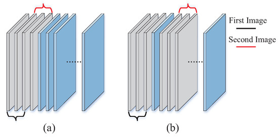
Figure 5.
Illustration of selecting 3-channel images from hyperspectral image on different interval D. (a) . (b) .
3.4. Classification Based on Vote Strategy
After feature extraction is completed, we input features into a common classifier SVM to achieve classification. This simple pattern of classification is more dependent on the discriminative capacity of the feature. The multi-scale feature has been proven practically to enhance discrimination [63]. The extraction of features at different scales was introduced in the last subsection. Directly concatenating them to obtain the multi-scale feature seems to be a conventional method of implementation, which is also incapable of achieving better classification results in our experimental attempt. Therefore, we aim to better utilize the discriminative capacity of features at different scales to achieve classification. A vote strategy is proposed for this purpose.
Benefiting from the near-real-time efficient training and classifying of SVM, we utilize SVM to implement multiple training runs and tests without significantly increasing time consumption. The feature at different scales can be defined as because interval D determines the scale of the final feature. Then, the () groups of features at different scales are concatenated with the original feature of HSI, respectively. The concatenated feature can be formulated as follows:
A multi-scale features set contains groups of different concatenated features , and k decides the number of . Different in set are utilized to construct training tasks, respectively, with the same training samples. Therefore, the corresponding prediction results from different trained SVM are combined to obtain . We vote for the final prediction labels. Specifically, for each predicted value sequence in , the predicted value with the most occurrence times is taken as the corresponding final predicted label of the sequence. When more than one category occurs the same number of times, the one that occurs first will be selected as result by default. With the vote strategy, the relatively prominent discrimination advantages of features at different scales can be utilized, and the classification errors can be smoothed, so as to improve the accuracy further. Its effectiveness will be demonstrated in the subsequent experimental section.
4. Results and Discussion
The environmental hardware is an Intel Core Intel (R) Xeon (R) Gold 6152 processor, 256G RAM and Nvidia A100 PCIE GPU. All the programs are developed with Python and Pytorch library.
4.1. Datasets and Evaluation Criterion
The video data involving FlyingChairs [55], FlyingChairs3D [64], and MPI-Sintel [39] datasets are used as source data for pre-training of PWC-Net, which is consistent with the original literature. Four open-source benchmark hyperspectral image scenes are selected as target data to demonstrate and analyze the effectiveness of the proposed method for the target task of feature extraction and classification. They are two rural scenes including Indian Pines, Salinas and two urban scenes including Pavia University, Houston 2013.
: This scene was photographed in North-Western Indiana by the Airborne Visible/Infrared Imaging Spectrometer (AVIRIS) sensor. It contains 200 bands from 0.4 μm to 2.5 μm, and it has an image size of with a 20 m spatial resolution. The gross number of ground categories in this scene is 16, and 10,776 samples are labeled artificially with expertise.
: This scene was photographed in Salinas Valley, California, by the Airborne Visible/Infrared Imaging Spectrometer (AVIRIS) sensor. It contains 204 bands from 0.4 μm to 2.5 μm, and it has an image size of with a 3.7 m spatial resolution. The gross number of ground categories in this scene is 16, and 54,129 samples are labeled artificially with expertise.
: This scene was photographed at Pavia University, Northern Italy, by the Reflective Optics System Imaging Spectrometer (ROSIS) sensor. It contains 103 bands from 0.43 μm to 0.86 μm, and it has an image size of with a 1.3 m spatial resolution. The gross number of ground categories in this scene is 9, and 42,776 samples are labeled artificially with expertise.
: This scene was photographed at Houston, South-Eastern Texas, by the ITRES CASI-1500 sensor in June 2012. It contains 144 bands from 0.38 μm to 1.05 μm, and it has an image size of with a 2.5 m spatial resolution. The gross number of ground categories in this scene is 15, and 15,029 samples are labeled artificially with expertise.
In order to demonstrate the performance of the proposed method under the condition of small samples classification, 10 training samples of each ground category are selected to compose the training dataset, and the rest of the labeled samples are utilized as the test dataset. To ensure the preciseness of the experiment, all experiments are repeated 10 times, and the results are averaged. In these 10 experiments, diverse groups of 10 training samples are selected to demonstrate the authentic performance of different methods under different sample distributions. Additionally, the selection of training samples in each iteration is completely identical by setting the same random number for all methods, which guarantees the fairness of comparison. Furthermore, the accuracy per category, the overall accuracy (OA), average accuracy (AA), and coefficient are taken as the evaluation criterion for evaluating the comprehensive performance of different approaches. Among them, the accuracy per category is just the percentage of the number of correctly classified samples of a category to the total number of samples of the category. OA denotes the percentage of the number of correctly classified samples in the total number of samples, which is used to evaluate the overall performance of the classification method. AA represents the average percentage of the number of correctly classified samples in each category in terms of the total number of samples in the category, which is used to evaluate the performance of the classification method for different categories. The coefficient adopts the discrete multivariate analysis method, which can provide a fairer evaluation of the classification method under the condition of the large uncertainty of classification results.
4.2. Implementation Details
The pre-training process of PWC-Net is carried out according to the original literature to obtain the optimal optical flow estimation capability. Specifically, the layer number of the pyramids extractor is set as L = 6, and the weights in the training loss function are set as = 0.32, = 0.08, = 0.02, = 0.01 and = 0.005. The trade-off weight is set to 0.0004. The calculation distance d of matching between the two pixels of two features in the cost volume layer is set to 3. The model is firstly trained on a FlyingChairs dataset with the initial learning rate 0.0001, and the cropped image size is . Then, the model is further trained on FlyingChairs3D dataset, and the cropped image size is . Finally, the MPI-Sintel dataset is utilized to fine-tune the model with data augmentation, and the cropped image size is also . So, the pre-training of the source network PWC-Net is achieved. Next, the pre-trained model can be transferred to the image-level feature extraction target task.
After completing feature extraction, the SVM is taken as the classifier. For SVM with a radial basis function (RBF) kernel, we utilize a cross-validation strategy to obtain the optimal regularization parameter and kernel parameter in the range of and , respectively.
4.3. Analysis of Vote Strategy
In order to verify the effectiveness of the voting strategy and analyze the discriminative capacity of image-level features at different scales, we set to observe the variation of classification performance as the interval D increases. The experimental results are shown in Table 1, and the results in the rows represent the mean ± standard deviation of 10 experiments under a specific setting. As we mentioned before, a different setting of interval D determines the presentation of variation information, so as to impact final image-level feature and classification performance. However, for different scenes, the optimal variation scale is not consistent. For example, the optimal scale is on the Indian Pines scene but on the Houston scene. It is not an intelligent choice to find the optimal scale to adapt to different scenes, while the vote strategy best utilizes the classification results of different variation scales to improve the ultimate accuracy. Simultaneously, it avoids the tedious search process for optimal parameters. Since increasing k cannot help to significantly improve classification performance, to balance efficiency and accuracy, we follow the setting of in the subsequent experiments.

Table 1.
The analysis results of overall accuracy with features at different scales and vote strategy.
4.4. Comparative Experiments
In order to conduct a comprehensive comparison with the proposed method, Spe-TL, we select seven open-source influential methods, including Extended Morphological Profiles (EMP) [8], Local Binary Patterns (LBP) [9], Deep Few-Shot Learning (DFSL) [31], 3D Convolutional Auto-Encoder (3D-CAE) [32], Spectral-Spatial Transformer Network (SSTN) [21], Patch-Free Global Learning Framework (FreeNet) [25], and CNN-Enhanced Graph Convolution Network (CEGCN) [65].
Among them, EMP and LBP are two representative traditional feature extraction methods. DFSL and 3D-CAE are two patch-level deep-learning-based feature extraction methods. DFSL, which aims for small samples classification, pre-trains its network on the source HSI data with sufficient labels, and it is fine-tuned using the target HSI data with limited labels. The 3D-CAE is capable of learning spatial–spectral features unsupervised on unlabeled HSI data when restoring the relevancy between output and input. The above mentioned feature extraction methods and our method all utilize the SVM for training and classification, so the discriminative capacity of features from different approaches can be directly compared. SSTN is an outstanding patch-level method which operates by introducing a transformer to replace the conventional convolution operations, and it is verified practically to perform better than other advanced influential patch-level methods such as SSAN [66], SSRN [17], etc. FreeNet and CEGCN are two representative image-level methods with better efficiency and accuracy than patch-level methods. FreeNet constructs the global learning network based on a fully convolution network that captures context information of a larger range. CEGCN combines the advantages of CNN in extracting local features and GCN in performing convolution operations in large-scale irregular regions, so as to achieve better performance than other advanced mainstream approaches based on CNN, such as FDSSC [67] and DBDA [68].
Table 2, Table 3, Table 4 and Table 5 quantitatively show the experimental results with all comparative approaches for the four scenes (only 10 training samples in each ground category); the results in the rows represent mean ± standard deviation of the 10 experiments under a specific setting. As we can observe, in the feature extraction approaches, the feature of DFSL aiming for small sample classification seems to have better discriminative power under the condition of only 10 training samples than 3D-CAE and the two traditional methods. The image-level feature of Spe-TL has the best feature discrimination. Additionally, its process of feature extraction is unsupervised, while DFSL requires HSI source data with a large number of labels when pre-training. The superior discriminative capability of Spe-TL also demonstrates the advantage of the image-level feature extraction methods compared with the patch-level. Furthermore, each of the deep-learning-based classification approaches has its advantages in a particular scene under the small sample condition. For example, SSTN performs relatively well on Indian Pines and Pavia University scenes but relatively poorly on Salinas and Houston scenes. FreeNet performs relatively well on Indian Pines and Salinas scenes but relatively poorly on the Pavia University scene. CEGCN performs relatively poorly on the two rural scenes while it achieves relatively higher accuracy for the two urban scenes. As for Spe-TL, it achieves the highest accuracy on all scenes and has an apparent increase in OA compared with CEGCN on two rural scenes (increases of 7.83%, and 5.00%, respectively). Therefore, Spe-TL was demonstrated to be capable of achieving competitive classification performances compared with the several influential deep-learning-based classification methods; furthermore, it had improved performance for the scenes containing an extensive range of planar ground objects, such as the rural scenes.
Table 2.
The analysis results of accuracy with different approaches on the Indian Pines scene (%) (10 training samples in each category).
Table 3.
The analysis results of accuracy with different approaches on the Salinas scene (%) (10 training samples in each category).
Table 4.
The analysis results of accuracy with different approaches on the Pavia University scene (%) (10 training samples in each category).
Table 5.
The analysis results of accuracy with different approaches on the Houston 2013 scene (%) (10 training samples in each category).
To focus on the analysis of single category, we used IP as an example to discuss the differences in accuracy per category. As we can see in Table 2, Spe-TL achieves the highest accuracy for the six categories of ground objects, including 2, 5, 11, 13, 14 and 16, which shows the advantage of Spe-TL in terms of accuracy per category. Additionally, Spe-TL also achieves results close to the highest in other categories of ground objects. However, as for categories 7 and 9, Spe-TL has a relatively poor performance because there are three methods, including SSTN, FreeNet, CEGCN that achieve an accuracy of 100%. Interestingly, other comparative methods also perform poorly for these two categories, which shows the difficulty of identifying them. Due to the transformer architecture of SSTN and patch-level input of FreeNet and CEGCN, these three methods perform well when capturing long-distance spatial information, which leads a better performance in categories 7 and 9 that is hard to distinguish merely with the spectral feature.
However, an approach with high accuracy may not produce a high-quality full-domain classification map, which doubtlessly weakens its practical application value. The accuracy is obtained by calculating only with labeled samples, while the full-domain classification map is obtained by classifying all sample including the labeled and the unlabeled elements. Therefore, the accuracy is not equal to the quality of the full-domain classification maps. A high-accuracy method only has practical value when it produces high quality classification maps. Therefore, we further produce the full-domain classification maps of different approaches with the four scenes to qualitatively and visually estimate their authentic performance, as shown in Figure 6, Figure 7, Figure 8 and Figure 9. As we can observe, except for LBP, the several feature-extraction-based methods utilizing SVM as a classifier can produce maps with clear category boundaries. However, a relatively low classification accuracy also results in numerous scatter noises that severely degrade the overall effect of the maps. As for LBP, although the texture feature can increase the classification accuracy, it is unable to produce practicable classification maps, which also verifies the conclusion mentioned above. Moreover, the several advanced deep-leaning-based classification methods with higher accuracy mitigate the noise phenomenon. Yet, some details are lost, and some category boundaries are blurred at the same time, which is mainly due to the smoothing effect of spatial information. Therefore, such problems lead to the classification map being slightly distorted compared to the original HSI, while Spe-TL better combines the advantages of both sides. On the one hand, the classification pattern of SVM guarantees the refined restoration of details. On the other hand, the powerful discriminative capacity of the image-level feature effectively decreases the number of noises so as to obtain a better visual effect. In order to demonstrate the ability of Spe-TL to restore details more clearly, we enlarge some areas on four scenes, as shown in Figure 6, Figure 7, Figure 8 and Figure 9. From these areas, we observe that Spe-TL can not only achieve accurate classification, but also subtly reflect the authentic distribution of ground objects compared with other methods. For example, on the Indian Pines scene, there are planar stone areas and a linear trees road located in the north, as well as a linear grass lane located in the middle. On the Salinas scene, there is a linear vinyard trellis path located in the south, and a linear romaine path and planar rough plow area located in the west. On the Pavia University scene, there is a planar roof of metal and asphalt located in the north. On the Houston scene, there is a planar roof of a circular commercial mall, planar soil, grass area, and linear road, which are located in the northwest.
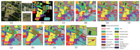
Figure 6.
The full-domain classification maps of different approaches on the Indian Pines scene: (a) False-color image. (b) Ground-truth map. (c) EMP. (d) LBP. (e) DFSL. (f) 3D-CAE. (g) SSTN. (h) FreeNet. (i) CEGCN. (j) Spe-TL.

Figure 7.
The full-domain classification maps of different approaches on the Salinas scene: (a) False-color image. (b) Ground-truth map. (c) EMP. (d) LBP. (e) DFSL. (f) 3D-CAE. (g) SSTN. (h) FreeNet. (i) CEGCN. (j) Spe-TL.
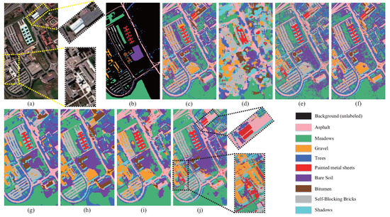
Figure 8.
The full-domain classification maps of different approaches on the Pavia University scene: (a) False-color image. (b) Ground-truth map. (c) EMP. (d) LBP. (e) DFSL. (f) 3D-CAE. (g) SSTN. (h) FreeNet. (i) CEGCN. (j) Spe-TL.
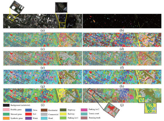
Figure 9.
The full-domain classification maps of different approaches on the Houston 2013 scene: (a) False-color image. (b) Ground-truth map. (c) EMP. (d) LBP. (e) DFSL. (f) 3D-CAE. (g) SSTN. (h) FreeNet. (i) CEGCN. (j) Spe-TL.
To further demonstrate the performance of the proposed method comprehensively, we continually increase the number of training samples in each category to 20, 50, 80, 100, 150, and 200; the performance variation trend of different approaches is shown in Figure 10. As we can observe, Spe-TL maintains an absolute superiority on the Indian Pines and Salinas scenes no matter how the training sample size varies. This fact again verifies the conclusion mentioned above that Spe-TL has improved performance on the scenes containing an extensive range of planar ground objects (Indian Pines, Salinas), which is due to the more distinct variation contained in the scenes and the more powerful discriminative capacity of image-level features. However, on other two urban scenes of Pavia University and Houston, Spe-TL does not gain a significant advantage with a varying sample size compared with advanced CEGCN. However, it still achieves competitive results with the highest accuracy. Simultaneously, as the number of training samples increases for these two scenes, the two image-level methods of FreeNet and CEGCN experience a degeneration in performance to different degrees, which indicates that the same increase in the number of bad samples limits the preferable fitting of the image-level network. However, for Spe-TL, no such limitation exists. Therefore, Spe-TL can achieve a performance that is competitive with the current state-of-the-art (SOTA) deep-learning-based methods regardless of how the training sample size varies.
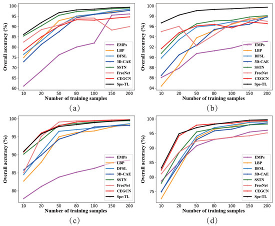
Figure 10.
The variation line graph of the overall accuracy of different approaches with a different number of training samples for four scenes. (a) Indian pines. (b) Salinas. (c) Pavia University. (d) Houston 2013.
Pursuing a more rounded comparison, we further compare Spe-TL with the existing HSI classification methods based on transfer learning, including 3D-LWNet [37], Two-CNN-transfer [30], HT-CNN-Attention [38], and CSDTL-MSA [36]. Since these methods are not open-source, we directly compare the results under certain experimental conditions in the original literature, as shown in Table 6. Because these methods also utilize the standard criterion of overall accuracy (OA) to indicate accuracy, we continue to use OA for comparison. The results in parentheses (·) are for Spe-TL under a completely consistent number of training samples on the target data. As we can observe, on multiple scenes and sample sizes, Spe-TL has a significant advantage over previous methods based on transfer learning, which demonstrates the superiority of our transfer learning strategy that transfers knowledge on optical flow estimation into an image-level feature extraction task. It also illustrates that our work is a novel and meaningful attempt.
Table 6.
The overall accuracy of different approaches based on transfer learning on the diverse scenes (%). The results in parentheses (·) are for the Spe-TL under the same number of training samples.
4.5. Analysis of Training and Inference Speed
For a meaningful comparison with Spe-TL, we select three representative methods with advanced performance for efficiency analysis, as shown in Table 7. Image-level methods FreeNet and CEGCN have a higher efficiency than the patch-level method of SSTN when training and testing. Additionally, the running time of image-level methods is not obviously extended with the expansion of training sample size, while the patch-level methods are opposite. Compared with other methods, the pre-trained Spe-TL helps to directly extract features of HSI so they can be classified without re-training, for which the running time is proportional to the image size and number of bands. Then, Spe-TL utilizes SVM for near-real-time efficient training and testing. Benefiting from this, a vote strategy that requires executing multiple training runs and tests is implemented, so the running time also increases (results in Table 7 are when and ). Even so, Spe-TL still has an advantage in efficiency and operation speed. Furthermore, it achieves near-real-time training and testing after extracting features as k further decreases. Therefore, Spe-TL is capable of quickly adapting to a new target HSI scene, which is more practical in application.
Table 7.
The running time of different approaches on the different scenes.
4.6. Analysis of Image-Level Feature
In this subsection, we explore the characteristics of image-level features by utilizing the visualization method. Firstly, the final presentation of the image-level feature is closely related with the global variation contained in each band. Therefore, we produce five groups of RGB images with an identical interval on all scenes, and each of them come from three consecutive single-band images in HSI. Additionally, the corresponding global variation information when extracting the feature is presented in optical flow diagrams, as shown in Figure 11. As mentioned above, we look at the HSI as a sequence of images. Therefore, for each of these images, the variation of the homogeneous region is similar while the variation of the heterogeneous region is distinguishable. The optical flow diagrams utilize different colors to represent the direction of spectral variation, i.e., similar colors denote the areas of approximately consistent variation at the current band. Moreover, the brightness of color is utilized to represent the degree of variation at an area with similar variation, i.e., the higher brightness denotes the more prominent variation. Such variation information is utilized to construct the final image-level feature that has greater discriminative power.
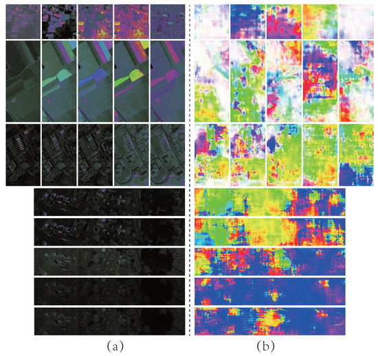
Figure 11.
Three consecutive single-band images on different scenes and the corresponding global variation information. (a) RGB images. (b) Optical Flow Diagrams.
The dimension-reduced-based T-SNE visualization method can map high-dimensional features to two-dimensional space, and can make features with a high similarity in a high-dimensional feature space with adjacent distance in a two-dimensional space. To further present the discriminative capacity of the image-level feature intuitively, we utilize the T-SNE visualization method to process features before and after extraction on different scenes, as shown in Figure 12. For a certain scene, different colored dots represent different categories of samples, and the distance between them in two-dimensional space can be approximately seen as the feature-similarity between them in a high-dimensional space. Except for the Indian Pines scene that only uses 600 samples per class because of the relatively small number of samples, all scenes select 1000 samples per class for visualization. As we can observe, the heterogeneous samples that overlap in the low-dimension space largely exist before feature extraction. This illustrates the high-similarity of original features, which makes them difficult to distinguish. Then, Spe-TL clearly enhances the distinguishable power of feature-by-feature extraction. This is reflected in the fact that homogeneous samples become more concentrated, and the distance between heterogeneous samples increases in low-dimensional space. Therefore, the image-level feature is more suitable for identification and classification.

Figure 12.
The T-SNE visualization results for the features before (first row) and after (second row) extracting on four scenes. (a) Indian pines. (b) Salinas. (c) Pavia University. (d) Houston 2013.
5. Conclusions
In this article, an image-level feature extraction method with transfer learning (Spe-TL) was proposed for HSI classification.
Several defects that exist in current deep learning methods and the successful practice of the image-level classification methods prompted us to attempt to research the special image-level feature extraction method with the transfer learning strategy. For this purpose, we bridge the gap between the HSI and video data, to successfully transfer the source network PWC-Net pre-trained on the video data to the hyperspectral feature extraction target task.
Our well-designed experiments on four open-source benchmark HSI scenes led to the following conclusions. (1) The proposed vote strategy best utilizes the classification results of different variation scales to improve the ultimate accuracy. (2) Spe-TL is capable of achieving a competitive classification performance compared with the current SOTA methods under various training sample sizes, and it has improved performance for the scenes containing an extensive range of planar ground objects such as the rural scenes. (3) Spe-TL produces detailed full-domain classification maps that subtly reflect the authentic distribution of ground objects. (4) After pre-training is completed, Spe-TL is capable of quickly adapting to the new target HSI scene, which is more practical in application.
Author Contributions
Methodology, B.L., Y.S.; investigation, A.Y. and K.G.; resources, A.Y. and K.G.; writing—original draft preparation, Y.S.; writing—review and editing, B.L., Y.S.; visualization, Y.S., L.D.; supervision, X.Y. All authors have read and agreed to the published version of the manuscript.
Funding
This research was funded by National Natural Science Foundation of China under Grant 41801388; Natural Science Foundation of Henan Province under Grant 222300420387.
Acknowledgments
The authors would like to thank the editors and reviewers for their constructive suggestions, which are significant contributions for our research work. We also thank the authors of PWC-Net for their work and contributions.
Conflicts of Interest
The authors declare no conflict of interest.
References
- Bioucas-Dias, J.M.; Plaza, A.; Camps-Valls, G.; Scheunders, P.; Nasrabadi, N.; Chanussot, J. Hyperspectral Remote Sensing Data Analysis and Future Challenges. IEEE Geosci. Remote Sens. Mag. 2013, 1, 6–36. [Google Scholar] [CrossRef]
- Zhong, Y.; Wang, X.; Xu, Y.; Wang, S.; Jia, T.; Hu, X.; Zhao, J.; Wei, L.; Zhang, L. Mini-UAV-Borne Hyperspectral Remote Sensing: From Observation and Processing to Applications. IEEE Geosci. Remote Sens. Mag. 2018, 6, 46–62. [Google Scholar] [CrossRef]
- Oquab, M.; Bottou, L.; Laptev, I.; Sivic, J. Learning and Transferring Mid-level Image Representations Using Convolutional Neural Networks. In Proceedings of the 2014 IEEE Conference on Computer Vision and Pattern Recognition, Columbus, OH, USA, 23–28 June 2014; pp. 1717–1724. [Google Scholar] [CrossRef]
- Sun, D.; Yang, X.; Liu, M.Y.; Kautz, J. PWC-Net: CNNs for Optical Flow Using Pyramid, Warping, and Cost Volume. In Proceedings of the 2018 IEEE/CVF Conference on Computer Vision and Pattern Recognition (CVPR), Salt Lake City, UT, USA, 18–22 June 2018. [Google Scholar]
- Camps-Valls, G.; Bruzzone, L. Kernel-based methods for hyperspectral image classification. IEEE Trans. Geosci. Remote Sens. 2005, 43, 1351–1362. [Google Scholar] [CrossRef]
- Agarwal, A.; El-Ghazawi, T.; El-Askary, H.; Le-Moigne, J. Efficient Hierarchical-PCA Dimension Reduction for Hyperspectral Imagery. In Proceedings of the 2007 IEEE International Symposium on Signal Processing and Information Technology, Cairo, Egypt, 15–18 December 2007; pp. 353–356. [Google Scholar] [CrossRef]
- Jia, S.; Hu, J.; Xie, Y.; Shen, L.; Jia, X.; Li, Q. Gabor Cube Selection Based Multitask Joint Sparse Representation for Hyperspectral Image Classification. IEEE Trans. Geosci. Remote Sens. 2016, 54, 3174–3187. [Google Scholar] [CrossRef]
- Fauvel, M.; Benediktsson, J.A.; Chanussot, J.; Sveinsson, J.R. Spectral and Spatial Classification of Hyperspectral Data Using SVMs and Morphological Profiles. IEEE Trans. Geosci. Remote Sens. 2008, 46, 3804–3814. [Google Scholar] [CrossRef]
- Li, W.; Chen, C.; Su, H.; Du, Q. Local Binary Patterns and Extreme Learning Machine for Hyperspectral Imagery Classification. IEEE Trans. Geosci. Remote Sens. 2015, 53, 3681–3693. [Google Scholar] [CrossRef]
- Xing, C.; Ma, L.; Yang, X. Stacked Denoise Autoencoder Based Feature Extraction and Classification for Hyperspectral Images. J. Sensors 2016, 2016, 1–10. [Google Scholar] [CrossRef]
- Hu, W.; Huang, Y.; Wei, L.; Zhang, F.; Li, H. Deep Convolutional Neural Networks for Hyperspectral Image Classification. J. Sensors 2015, 2015, 1687-725X. [Google Scholar] [CrossRef]
- Chen, Y.; Zhu, L.; Ghamisi, P.; Jia, X.; Li, G.; Tang, L. Hyperspectral Images Classification With Gabor Filtering and Convolutional Neural Network. IEEE Geosci. Remote Sens. Lett. 2017, 14, 2355–2359. [Google Scholar] [CrossRef]
- Liu, B.; Yu, X.; Zhang, P.; Yu, A.; Fu, Q.; Wei, X. Supervised Deep Feature Extraction for Hyperspectral Image Classification. IEEE Trans. Geosci. Remote Sens. 2018, 56, 1909–1921. [Google Scholar] [CrossRef]
- Chen, Y.; Jiang, H.; Li, C.; Jia, X.; Ghamisi, P. Deep Feature Extraction and Classification of Hyperspectral Images Based on Convolutional Neural Networks. IEEE Trans. Geosci. Remote Sens. 2016, 54, 6232–6251. [Google Scholar] [CrossRef]
- Liu, B.; Yu, X.; Zhang, P.; Tan, X. Deep 3D convolutional network combined with spatial-spectral features for hyperspectral image classification. Acta Geod. Cartogr. Sin. 2019, 48, 53. [Google Scholar]
- Lin, Z.; Chen, Y.; Ghamisi, P.; Benediktsson, J.A. Generative Adversarial Networks for Hyperspectral Image Classification. IEEE Trans. Geosci. Remote Sens. 2018, 56, 5046–5063. [Google Scholar]
- Zhong, Z.; Li, J.; Luo, Z.; Chapman, M. Spectral–spatial residual network for hyperspectral image classification: A 3-D deep learning framework. IEEE Trans. Geosci. Remote Sens. 2017, 56, 847–858. [Google Scholar] [CrossRef]
- Tang, X.; Meng, F.; Zhang, X.; Cheung, Y.M.; Ma, J.; Liu, F.; Jiao, L. Hyperspectral Image Classification Based on 3-D Octave Convolution With Spatial–Spectral Attention Network. IEEE Trans. Geosci. Remote Sens. 2021, 59, 2430–2447. [Google Scholar] [CrossRef]
- Gao, K.; Liu, B.; Yu, X.; Zhang, P.; Sun, Y. Small sample classification of hyperspectral image using model-agnostic meta-learning algorithm and convolutional neural network. Int. J. Remote Sens. 2021, 42, 3090–3122. [Google Scholar] [CrossRef]
- Paoletti, M.E.; Haut, J.M.; Fernandez-Beltran, R.; Plaza, J.; Plaza, A.; Li, J.; Pla, F. Capsule Networks for Hyperspectral Image Classification. IEEE Trans. Geosci. Remote Sens. 2019, 57, 2145–2160. [Google Scholar] [CrossRef]
- Zhong, Z.; Li, Y.; Ma, L.; Li, J.; Zheng, W.S. Spectral–Spatial Transformer Network for Hyperspectral Image Classification: A Factorized Architecture Search Framework. IEEE Trans. Geosci. Remote Sens. 2022, 60, 1–15. [Google Scholar] [CrossRef]
- Hong, D.; Han, Z.; Yao, J.; Gao, L.; Zhang, B.; Plaza, A.; Chanussot, J. SpectralFormer: Rethinking Hyperspectral Image Classification With Transformers. IEEE Trans. Geosci. Remote Sens. 2022, 60, 1–15. [Google Scholar] [CrossRef]
- Shen, Y.; Zhu, S.; Chen, C.; Du, Q.; Xiao, L.; Chen, J.; Pan, D. Efficient Deep Learning of Nonlocal Features for Hyperspectral Image Classification. IEEE Trans. Geosci. Remote Sens. 2020, 59, 6029–6043. [Google Scholar] [CrossRef]
- Xu, Y.; Du, B.; Zhang, L. Beyond the Patchwise Classification: Spectral-Spatial Fully Convolutional Networks for Hyperspectral Image Classification. IEEE Trans. Big Data 2020, 6, 492–506. [Google Scholar] [CrossRef]
- Zheng, Z.; Zhong, Y.; Ma, A.; Zhang, L. FPGA: Fast Patch-Free Global Learning Framework for Fully End-to-End Hyperspectral Image Classification. IEEE Trans. Geosci. Remote Sens. 2020, 58, 5612–5626. [Google Scholar] [CrossRef]
- Wang, D.; Du, B.; Zhang, L. Fully Contextual Network for Hyperspectral Scene Parsing. IEEE Trans. Geosci. Remote Sens. 2021, 60, 1–16. [Google Scholar] [CrossRef]
- Wang, Y.; Li, K.; Xu, L.; Wei, Q.; Wang, F.; Chen, Y. A Depthwise Separable Fully Convolutional ResNet With ConvCRF for Semisupervised Hyperspectral Image Classification. IEEE J. Sel. Top. Appl. Earth Obs. Remote Sens. 2021, 14, 4621–4632. [Google Scholar] [CrossRef]
- Jiang, G.; Sun, Y.; Liu, B. A fully convolutional network with channel and spatial attention for hyperspectral image classification. Remote Sens. Lett. 2021, 12, 1238–1249. [Google Scholar] [CrossRef]
- Sun, Y.; Liu, B.; Yu, X.; Yu, A.; Xue, Z.; Gao, K. Resolution reconstruction classification: Fully octave convolution network with pyramid attention mechanism for hyperspectral image classification. Int. J. Remote Sens. 2022, 43, 2076–2105. [Google Scholar] [CrossRef]
- Yang, J.; Zhao, Y.Q.; Chan, J.C.W. Learning and Transferring Deep Joint Spectral–Spatial Features for Hyperspectral Classification. IEEE Trans. Geosci. Remote Sens. 2017, 55, 4729–4742. [Google Scholar] [CrossRef]
- Liu, B.; Yu, X.; Yu, A.; Zhang, P.; Wan, G.; Wang, R. Deep Few-Shot Learning for Hyperspectral Image Classification. IEEE Trans. Geosci. Remote Sens. 2019, 57, 2290–2304. [Google Scholar] [CrossRef]
- Mei, S.; Ji, J.; Geng, Y.; Zhang, Z.; Li, X.; Du, Q. Unsupervised Spatial–Spectral Feature Learning by 3D Convolutional Autoencoder for Hyperspectral Classification. IEEE Trans. Geosci. Remote Sens. 2019, 57, 6808–6820. [Google Scholar] [CrossRef]
- Liu, B.; Yu, A.; Yu, X.; Wang, R.; Gao, K.; Guo, W. Deep Multiview Learning for Hyperspectral Image Classification. IEEE Trans. Geosci. Remote Sens. 2021, 59, 7758–7772. [Google Scholar] [CrossRef]
- Zhang, J.; Li, W.; Ogunbona, P.; Xu, D. Recent Advances in Transfer Learning for Cross-Dataset Visual Recognition: A Problem-Oriented Perspective. ACM Comput. Surv. (CSUR) 2019, 52, 1–38. [Google Scholar] [CrossRef]
- Windrim, L.; Melkumyan, A.; Murphy, R.J.; Chlingaryan, A.; Ramakrishnan, R. Pretraining for Hyperspectral Convolutional Neural Network Classification. IEEE Trans. Geosci. Remote Sens. 2018, 56, 2798–2810. [Google Scholar] [CrossRef]
- Zhong, C.; Zhang, J.; Wu, S.; Zhang, Y. Cross-Scene Deep Transfer Learning With Spectral Feature Adaptation for Hyperspectral Image Classification. IEEE J. Sel. Top. Appl. Earth Obs. Remote Sens. 2020, 13, 2861–2873. [Google Scholar] [CrossRef]
- Zhang, H.; Li, Y.; Jiang, Y.; Wang, P.; Shen, Q.; Shen, C. Hyperspectral Classification Based on Lightweight 3-D-CNN With Transfer Learning. IEEE Trans. Geosci. Remote Sens. 2019, 57, 5813–5828. [Google Scholar] [CrossRef]
- He, X.; Chen, Y.; Ghamisi, P. Heterogeneous Transfer Learning for Hyperspectral Image Classification Based on Convolutional Neural Network. IEEE Trans. Geosci. Remote Sens. 2020, 58, 3246–3263. [Google Scholar] [CrossRef]
- Butler, D.J.; Wulff, J.; Stanley, G.B.; Black, M.J. A Naturalistic Open Source Movie for Optical Flow Evaluation. In Computer Vision—ECCV 2012; Fitzgibbon, A., Lazebnik, S., Perona, P., Sato, Y., Schmid, C., Eds.; Springer: Berlin/Heidelberg, Germany, 2012; pp. 611–625. [Google Scholar]
- Xiao, X.; Hu, H.; Wang, W. Trajectories-based motion neighborhood feature for human action recognition. In Proceedings of the 2017 IEEE International Conference on Image Processing (ICIP), Beijing, China, 17–20 September 2017; pp. 4147–4151. [Google Scholar] [CrossRef]
- Ochs, P.; Malik, J.; Brox, T. Segmentation of Moving Objects by Long Term Video Analysis. IEEE Trans. Pattern Anal. Mach. Intell. 2014, 36, 1187–1200. [Google Scholar] [CrossRef] [PubMed]
- Menze, M.; Geiger, A. Object scene flow for autonomous vehicles. In Proceedings of the 2015 IEEE Conference on Computer Vision and Pattern Recognition (CVPR), Boston, MA, USA, 7–12 June 2015; pp. 3061–3070. [Google Scholar] [CrossRef]
- Horn, B.; Schunck, B.G. Determining Optical Flow. In Techniques and Applications of Image Understanding; SPIE: Bellingham, DC, USA, 1981. [Google Scholar]
- Brox, T.; Bruhn, A.; Papenberg, N.; Weickert, J. High Accuracy Optical Flow Estimation Based on a Theory for Warping. In Proceedings of the European Conference on Computer Vision, Prague, Czech Republic, 11–14 May 2004. [Google Scholar]
- Papenberg, N.; Bruhn, A.; Brox, T.; Didas, S.; Weickert, J. Highly Accurate Optic Flow Computation with Theoretically Justified Warping. Int. J. Comput. Vis. 2006, 67, 141–158. [Google Scholar] [CrossRef]
- Sun, D.; Roth, S.; Black, M.J. Secrets of Optical Flow Estimation and Their Principles. In Proceedings of the Twenty-Third IEEE Conference on Computer Vision and Pattern Recognition (CVPR), San Francisco, CA, USA, 13–18 June 2010. [Google Scholar]
- Baker, S.; Scharstein, D.; Lewis, J.P.; Roth, S.; Black, M.J.; Szeliski, R. A Database and Evaluation Methodology for Optical Flow. Int. J. Comput. Vis. 2011, 92, 1–31. [Google Scholar] [CrossRef]
- Vogel, C.; Roth, S.; Schindler, K. An Evaluation of Data Costs for Optical Flow. In Proceedings of the German Conference on Pattern Recognition, Saarbrücken, Germany, 4–6 September 2013. [Google Scholar]
- Brox, T.; Malik, J. Large Displacement Optical Flow: Descriptor Matching in Variational Motion Estimation. IEEE Trans. Pattern Anal. Mach. Intell. 2011, 33, 500–513. [Google Scholar] [CrossRef]
- Barnes, C.; Shechtman, E.; Dan, B.G.; Finkelstein, A. The Generalized PatchMatch Correspondence Algorithm. In Proceedings of the European Conference on Computer Vision, Heraklion, Crete, Greece, 5–11 September 2010. [Google Scholar]
- Liu, C.; Yuen, J.; Torralba, A. SIFT Flow: Dense Correspondence across Scenes and Its Applications. IEEE Trans. Pattern Anal. Mach. Intell. 2011, 33, 978–994. [Google Scholar] [CrossRef]
- Weinzaepfel, P.; Revaud, J.; Harchaoui, Z.; Schmid, C. DeepFlow: Large Displacement Optical Flow with Deep Matching. In Proceedings of the 2013 IEEE International Conference on Computer Vision, Sydney, Australia, 1–8 December 2013; pp. 1385–1392. [Google Scholar] [CrossRef]
- Gadot, D.; Wolf, L. PatchBatch: A Batch Augmented Loss for Optical Flow. In Proceedings of the 2016 IEEE Conference on Computer Vision and Pattern Recognition (CVPR), Las Vegas, NV, USA, 27–30 June 2016; pp. 4236–4245. [Google Scholar] [CrossRef]
- Han, X.; Leung, T.; Jia, Y.; Sukthankar, R.; Berg, A.C. MatchNet: Unifying feature and metric learning for patch-based matching. In Proceedings of the 2015 IEEE Conference on Computer Vision and Pattern Recognition (CVPR), Boston, MA, USA, 7–12 June 2015; pp. 3279–3286. [Google Scholar] [CrossRef]
- Dosovitskiy, A.; Fischer, P.; Ilg, E.; Häusser, P.; Hazirbas, C.; Golkov, V.; Smagt, P.v.d.; Cremers, D.; Brox, T. FlowNet: Learning Optical Flow with Convolutional Networks. In Proceedings of the 2015 IEEE International Conference on Computer Vision (ICCV), Santiago, Chile, 7–13 December 2015; pp. 2758–2766. [Google Scholar] [CrossRef]
- Ilg, E.; Mayer, N.; Saikia, T.; Keuper, M.; Dosovitskiy, A.; Brox, T. FlowNet 2.0: Evolution of Optical Flow Estimation with Deep Networks. In Proceedings of the 2017 IEEE Conference on Computer Vision and Pattern Recognition (CVPR), Honolulu, HI, USA, 21–26 July 2017; pp. 1647–1655. [Google Scholar] [CrossRef]
- Ranjan, A.; Black, M.J. Optical Flow Estimation Using a Spatial Pyramid Network. In Proceedings of the 2017 IEEE Conference on Computer Vision and Pattern Recognition (CVPR), Honolulu, HI, USA, 21-26 July 2017; pp. 2720–2729. [Google Scholar] [CrossRef]
- Hui, T.W.; Tang, X.; Loy, C.C. LiteFlowNet: A Lightweight Convolutional Neural Network for Optical Flow Estimation. In Proceedings of the 2018 IEEE/CVF Conference on Computer Vision and Pattern Recognition, Salt Lake City, UT, USA, 18–22 June 2018; pp. 8981–8989. [Google Scholar] [CrossRef]
- Janai, J.; Güney, F.; Ranjan, A.; Black, M.; Geiger, A. Unsupervised Learning of Multi-Frame Optical Flow with Occlusions. In Proceedings of the European Conference on Computer Vision, Munich, Germany, 8–14 September 2018. [Google Scholar]
- Liu, P.; Lyu, M.; King, I.; Xu, J. SelFlow: Self-Supervised Learning of Optical Flow. In Proceedings of the 2019 IEEE/CVF Conference on Computer Vision and Pattern Recognition (CVPR), Long Beach, CA, USA, 15–20 June 2019; pp. 4566–4575. [Google Scholar] [CrossRef]
- Tian, L.; Tu, Z.; Zhang, D.; Liu, J.; Li, B.; Yuan, J. Unsupervised Learning of Optical Flow With CNN-Based Non-Local Filtering. IEEE Trans. Image Process. 2020, 29, 8429–8442. [Google Scholar] [CrossRef]
- Sun, D.; Roth, S.; Michael, J. A Quantitative Analysis of Current Practices in Optical Flow Estimation and the Principles Behind Them. Kluwer Acad. Publ. 2014, 106, 115–137. [Google Scholar]
- Zhang, C.; Li, G.; Du, S. Multi-Scale Dense Networks for Hyperspectral Remote Sensing Image Classification. IEEE Trans. Geosci. Remote Sens. 2019, 57, 9201–9222. [Google Scholar] [CrossRef]
- Mayer, N.; Ilg, E.; Häusser, P.; Fischer, P.; Cremers, D.; Dosovitskiy, A.; Brox, T. A Large Dataset to Train Convolutional Networks for Disparity, Optical Flow, and Scene Flow Estimation. In Proceedings of the 2016 IEEE Conference on Computer Vision and Pattern Recognition (CVPR), Las Vegas, NV, USA, 27–30 June 2016; pp. 4040–4048. [Google Scholar] [CrossRef]
- Liu, Q.; Xiao, L.; Yang, J.; Wei, Z. CNN-Enhanced Graph Convolutional Network With Pixel- and Superpixel-Level Feature Fusion for Hyperspectral Image Classification. IEEE Trans. Geosci. Remote Sens. 2021, 59, 8657–8671. [Google Scholar] [CrossRef]
- Sun, H.; Zheng, X.; Lu, X.; Wu, S. Spectral–Spatial Attention Network for Hyperspectral Image Classification. IEEE Trans. Geosci. Remote Sens. 2020, 58, 3232–3245. [Google Scholar] [CrossRef]
- Wang, W.; Dou, S.; Jiang, Z.; Sun, L. A Fast Dense Spectral–Spatial Convolution Network Framework for Hyperspectral Images Classification. Remote Sens. 2018, 10, 1068. [Google Scholar] [CrossRef]
- Li, R.; Zheng, S.; Duan, C.; Yang, Y.; Wang, X. Classification of Hyperspectral Image Based on Double-Branch Dual-Attention Mechanism Network. Remote Sens. 2020, 12, 582. [Google Scholar] [CrossRef]


Publisher’s Note: MDPI stays neutral with regard to jurisdictional claims in published maps and institutional affiliations. |
© 2022 by the authors. Licensee MDPI, Basel, Switzerland. This article is an open access article distributed under the terms and conditions of the Creative Commons Attribution (CC BY) license (https://creativecommons.org/licenses/by/4.0/).