Impact of Atmospheric Correction Methods Parametrization on Soil Organic Carbon Estimation Based on Hyperion Hyperspectral Data

Abstract

Visible Near infrared and Shortwave Infrared (VNIR/SWIR, 400–2500 nm) remote sensing data is becoming a tool for topsoil properties mapping, bringing spatial information for environmental modeling and land use management. These topsoil properties estimates are based on regression models, linking a key topsoil property to VNIR/SWIR reflectance data. Therefore, the regression model’s performances depend on the quality of both topsoil property analysis (measured on laboratory over-ground soil samples) and Bottom-of-Atmosphere (BOA) VNIR/SWIR reflectance which are retrieved from Top-Of-Atmosphere radiance using atmospheric correction (AC) methods. This paper examines the sensitivity of soil organic carbon (SOC) estimation to BOA images depending on two parameters used in AC methods: aerosol optical depth (AOD) in the FLAASH (Fast Line-of-Sight Atmospheric Analysis of Spectral Hypercubes) method and water vapor (WV) in the ATCOR (ATmospheric CORrection) method. This work was based on Earth Observing-1 Hyperion Hyperspectral data acquired over a cultivated area in Australia in 2006. Hyperion radiance data were converted to BOA reflectance using seven values of AOD (from 0.2 to 1.4) and six values of WV (from 0.4 to 5 cm), in FLAASH and ATCOR, respectively. Then a Partial Least Squares regression (PLSR) model was built from each Hyperion BOA data to estimate SOC over bare soil pixels. This study demonstrated that the PLSR models were insensitive to the AOD variation used in the FLAASH method, with R²_cv and RMSE_cv of 0.79 and 0.4%, respectively. The PLSR models were slightly sensitive to the WV variation used in the ATCOR method, with R²_cv ranging from 0.72 to 0.79 and RMSE_cv ranging from 0.41 to 0.47. Regardless of the AOD values, the PLSR model based on the best parametrization of the ATCOR model provided similar SOC prediction accuracy to PLSR models using the FLAASH method. Variation in AOD using the FLAASH method did not impact the identification of bare soil pixels coverage which corresponded to 82.35% of the study area, while a variation in WV using the ATCOR method provided a variation of bare soil pixels coverage from 75.04 to 84.04%. Therefore, this work recommends (1) the use of the FLAASH AC method to provide BOA reflectance values from Earth Observing-1 Hyperion Hyperspectral data before SOC mapping or (2) a careful selection of the WV parameter when using ATCOR.

1. Introduction

Soil is a heterogeneous composite material with a wide range of physical and chemical properties. It supports life and vegetation on earth and plays a central role in many of today’s environmental challenges. A solid understanding of soil is required for improved soil management. Composition and properties such as clay, sand, silt, calcium carbonate, free iron, organic carbon, and pH in the spatial and temporal domains. Soil organic carbon (SOC) is one of the major soil constituents because of its ability to influence plant growth as a source of energy and a trigger for nutrient availability via mineralization [1]. SOC is also important for the carbon cycle in terrestrial environments [2]. The determination of SOC content is also an obvious requirement to determine the rate and/or extent of Carbon soil sequestration. In agronomy, soil science, and climate change research, information on geographical and temporal fluctuations in SOC content is needed [3,4]. Traditional laboratory procedures for determining SOC content are time-consuming, expensive, and labor-intensive. The VNIR/SWIR spectroscopy (350–2500 µm) can be used to estimate the SOC in lab, field and from remote sensing conditions [5]. The soil reflectance spectra in the 1100–2500 nm range generally includes three distinct absorption peaks around 1400, 1900, and 2200 nm with a few small absorption peaks between 2200 and 2500 nm [6]. The effect of SOC containing biochemical constituents like chlorophyll, oil, cellulose, pectin, starch, lignin, and humic acids [7] is dominant in the visible and near infra-red portion of the spectrum (400–1100 nm), and some parts of the SWIR region (1100–2500 nm) [8], and soil reflectance generally decreases with organic matter content [9]. Simple Linear Regression [10], Principal Component Analysis [11], Partial Least Squares regression (PLSR) [12], and Artificial Neural Networks [13] are some of the statistical techniques used for SOC estimation. Out of these methods, PLSR is the most common method. VNIR/SWIR hyperspectral remote sensing data were becoming a potential tool to extend SOC mapping [14,15]. However, this technique is affected by the presence of green and dry vegetation [16,17], topsoil moisture [18] and atmospheric composition [19]. Concerning the latter, since the mid-1980s some Atmospheric Correction (AC) methods have been developed which were applied on VNIR/SWIR data obtained via airborne and spaceborne multispectral and hyperspectral sensors. AC methods are used to convert the Top-Of-Atmosphere radiance to the surface reflectance (also called Bottom-of-Atmosphere reflectance). By reducing external atmospheric components, reflectance can be improved. Empirical models, radiative transfer models, and hybrid models are the three categories of AC models. They have evolved from an empirical approach to rigorous radiative transfer modeling [20].

Empirical models mainly rely on image statistics to estimate surface reflectance. A few of the empirical methods are Internal Average Reflectance (IAR), Flat Field (FF), and Empirical line method [21]. Darkest Pixel principle (DP) is also an empirical method, where studies [22] indicated the best results for accurate surface reflectance estimation are achieved using a method that adds the effect of Rayleigh scattering to conventional dark object subtraction. For atmospheric correction and aerosol retrieval, semi-empirical approaches such as QUick atmospheric correction (QUAC) [23] are used. Radiative transfer methods simulate the absorption and scattering effects of atmospheric components. To mimic the atmosphere, several algorithms have been created, notably ATREM (ATmospheric REMoval algorithm), ATCOR (ATmospheric CORrection [24], FLAASH (Fast Line-of-sight Atmospheric Analysis of Spectral Hypercubes [25], ISDAS (Imaging Spectrometer Data Analysis System [26], HATCH (High-accuracy ATmosphere Correction for Hyperspectral data [27], and ACORN (Atmospheric CORrection Now) [28]. For the derivation of surface reflectance from hyperspectral imaging data, hybrid models commonly combine radiative modeling with empirical methodologies. With physical models, Gordon [29] has summarized the evolution of Ocean color Atmospheric corrections right from its early years to the current scenarios. Other physical models are also developed and used for various applications [30,31]

Some studies compared performances of AC models for identifying tree species [32], mineral mapping [33], littoral environments studies [34], and SOC content mapping [35]. Beyond the type of AC methods and the choice of the AC method, the atmospheric parameters (e.g., Aerosol Optical Depth, Water vapor, Ozone, Visibility) used in AC methods might be uncertain and the choice of these atmospheric parameters may impact the reflectance quality. Only a few studies focused on an evaluation of the impacts of these atmospheric parameters on reflectance quality such as ozone, water vapor, Rayleigh scattering, aerosol scattering on the spectral reflectance of NOAA-AVHRR and derived NDVI data [36,37]. Mannschatz et al. [38] studied sensitivity of LAI estimation from satellite imaging to atmospheric correction using ATCOR, and highlighted that the ATCOR parameter ‘visibility’ has the strongest influence on LAI estimation. Griffin et al. [39] studied the sensitivity of Visibility, Aerosol model type, Atmospheric model and solar zenith on surface reflectance using AVIRIS data in FLAASH and ATREM and concluded the sensitivity to input visibility generally varied between +0.03 for both AC models. Davaadorj. A. [40] studied the sensitivity of different aerosol models using Worldview 3 data with FLAASH and ATCOR AC and concluded that maritime aerosol has the least sensitivity compared to rural and urban models. The variation of surface reflectance caused by different surface types such as sand, artificial turf, grass, bright and dark targets with respect to AOD was studied by Nazer et al. and Bassani et al. [41,42].

In this context, the aim of the study is to evaluate the uncertainty of SOC prediction due to two atmospheric parameters used in AC methods: the water vapor (WV) using ATCOR and the Aerosol Optical Depth (AOD) using FLAASH. A Hyperspectral Hyperion image was corrected by ATCOR and FLAASH AC methods to convert the at-sensor radiance spectrum to the ground reflectance spectrum, with a feasible range of WV and AOD values, respectively. And the PLSR method was selected as the classical chemometric method for SOC content estimation based on each corrected Hyperion reflectance data. The data and methods used are presented in Section 2 and the results in Section 3. Finally, the results are discussed in Section 4.

2. Materials and Methods

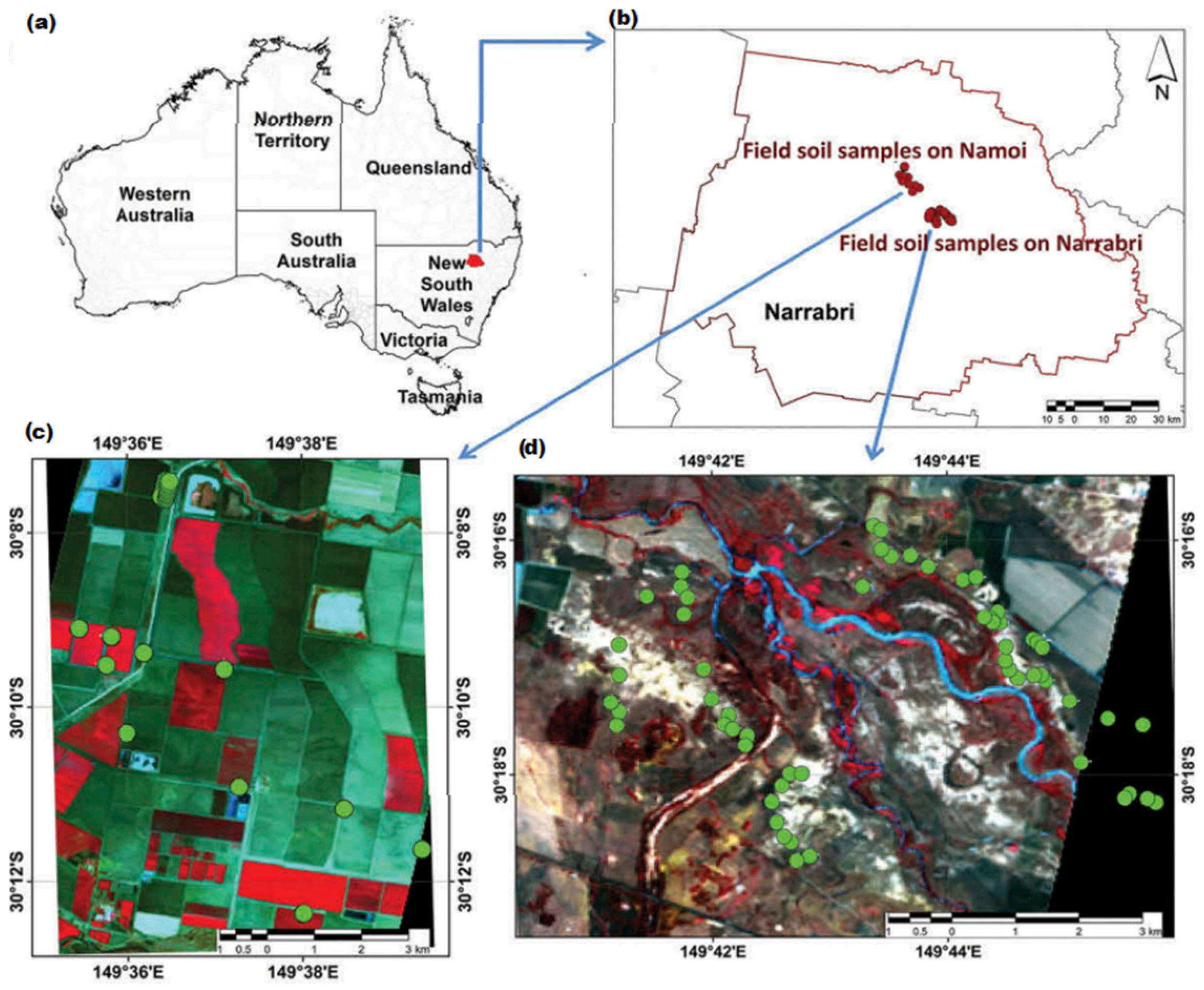
2.1. Study Area

The Narrabri site is in Australia’s northwestern state of New South Wales (NSW) (Figure 1a). The study area is divided into two subsites: the cotton fields of Namoi (referred to as Narrabri site#1 henceforth) (149°37′E, 30°10′S), which cover 70 km², and the pastures in the town of Narrabri (referred to as Narrabri site#2), which covers 69 km² (Figure 1b). The Australian fields are extensive and continuous (approximately 500 m × 900 m). Vertisols predominate in this area. The terrain is flat, with plane regions rising to an average elevation of 210 m above sea level.

2.2. Raw Hyperion Data

The EO-1 satellite’s Hyperion sensor monitors radiation from 400 to 2500 nm in 242 spectral bands with a spectral resolution of about 10 nm and a spatial resolution of 30 m. The Hyperion images have a sweep width of 7.6 km. Folkman et al. [43] provided a full description of Hyperion’s characteristics, operations, and uses.

Two Hyperion cloud-free pictures were obtained over the Narrabri study area in this study: the first on 13 December 2006 at 23:51 UT over Narrabri pasture soils (site#2), and the second on 17 January 2007 at 23:47 UT over cropping soils (site#1) and traveling stock routes of Namoi. The Hyperion images were georeferenced Hyperion images in L1T format (Figure 1c,d).

2.3. Soil Sampling

Over the two Narrabri locations, a total of 98 soil samples were collected (Figure 1c,d) from researchers of The University of Sydney in Australia [12]. It includes 46 samples from Narrabri site#1’s cropping soils and stock routes collected in October 2006 (during the same semester as Hyperion data) (Figure 1c) and 52 samples from Narrabri site#2’s pastures collected in December 2006 (during the same month as Hyperion data) (Figure 1d). During the field campaign, soil samples were gathered from bare soil areas. Because there was no organic matter added or consumed in the field due to the absence of vegetation during this period at the sampling locations, SOC content may be deemed steady between sampling and picture collection. Climate change, particularly changes in temperature and rainfall, have an impact on SOC by hastening its decomposition. However, it was reliably concluded that SOC was very consistent between measurements in Narrabri site#1 during a short period of three months from October 2006 to January 2007. Soil samples were taken at a depth of 0 to 10 cm. This depth corresponds to the ploughed soil horizon, and the Hyperion measurement may be deemed indicative of this tested depth because the soil samples were gathered on cultivated areas. Soil samples are the average of sub-samples obtained at the center and four corners of a 20 × 20 m area’s perimeter.

2.4. SOC Laboratory Measurements

Laboratory mid-infrared (MIR) spectroscopy was used to determine the SOC content of soil samples. Samples were crushed to 200 μm for MIR analysis and analyzed as neat powders. Each soil sample’s MIR spectral reflectance was measured using a Bruker Optics Tensor 37 Fourier Transform Infrared spectrometer with an 8 cm-1 resolution and 64 scans per second in the range 2500 to 25,000 nm. PLSR from MIR calibrations was used to predict the SOC content of each soil sample [12]. The calibration used 13 factors, and the model’s root mean squared error in the test set validation was 0.15 dag/kg, with an R² of 0.91 [12]. The SOC ranges from 0.002% to 3.6%, with a mean of 1.56%, and a standard deviation of 0.97%.

2.5. Atmospheric Parameters

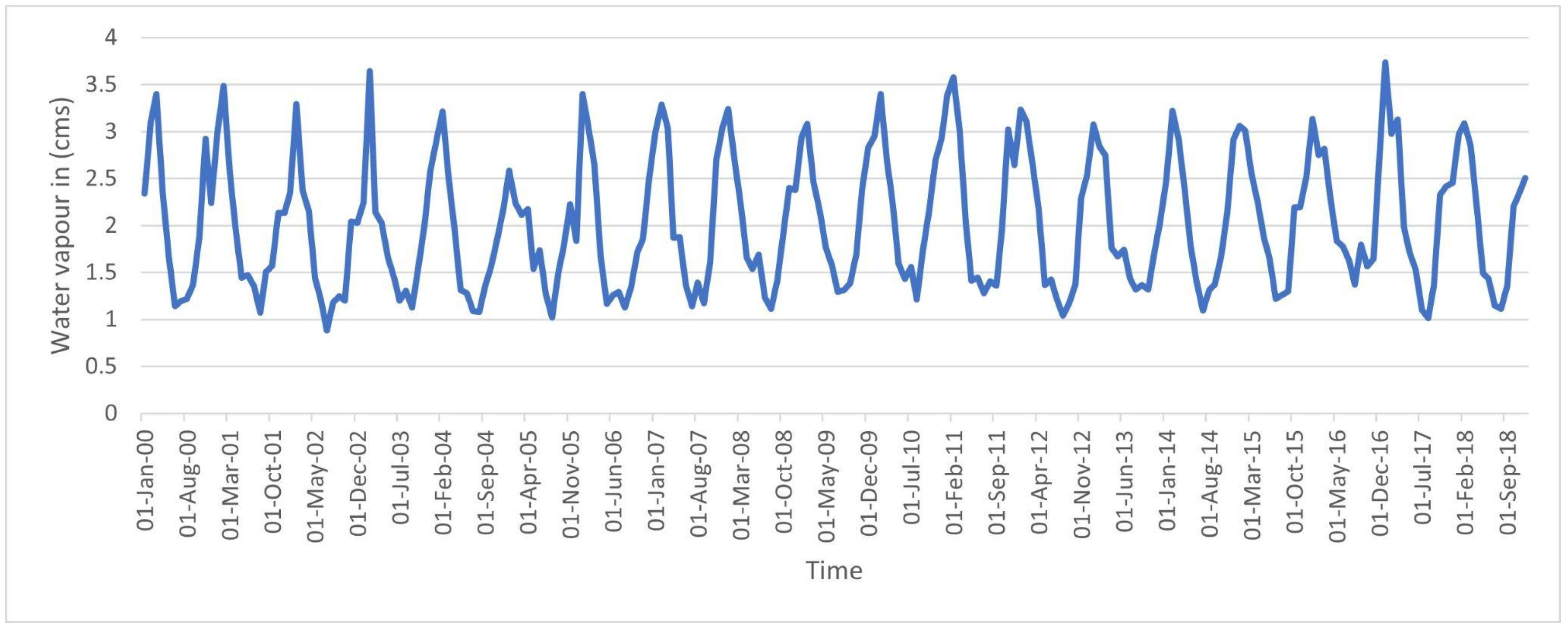
2.5.1. Water Vapor

Water vapor (WV) absorption has a strong effect within specific absorption bands, but spectral bands for land surface observations are typically designed to avoid strong absorption lines. Hence water vapor absorption must be accurately corrected in the selected bands. From a joint project between the National Center for Environmental Prediction (NCEP, formerly “NMC”) and the National Center for Atmospheric Research (NCAR) [44], the total column WV over the study area ranged between 0.9 cm to 3.7 cm in the last 15 years (from 2000 to 2015, Figure 2,

Table 1. WV and AOD estimations, estimated by the joint project between the National Centers for Environmental Prediction (NCEP, formerly “NMC”), the National Center for Atmospheric Research (NCAR), and the atmosphere global product based on Modis MOD08_M3 V6, respectively.

	Water Vapor (WV) (in cm)	Aerosol Optical Depth (AOD)
Minimum	0.9	0.02
Maximum	3.7	1.50
Mean	2	0.48
Median	1.9	0.42
Standard Deviation	0.7	0.25

). These WV values were estimated by reanalysis models built from historic meteorological data collected over 15 years.

At the date of the Hyperion images acquisition, the total column WV value would be estimated between 2.8 cm and 3.1 cm. Finally, considering the “Mid Latitude Summer” climatic condition over the study area, the default WV value usually selected in the ATCOR model would be 2–3 cm (Table 3, [12]). The Hyperion data were corrected from atmospheric effects using six WV values, preselected by the ATCOR software: 0.4, 1, 2, 2.9, 4, and 5 cm.

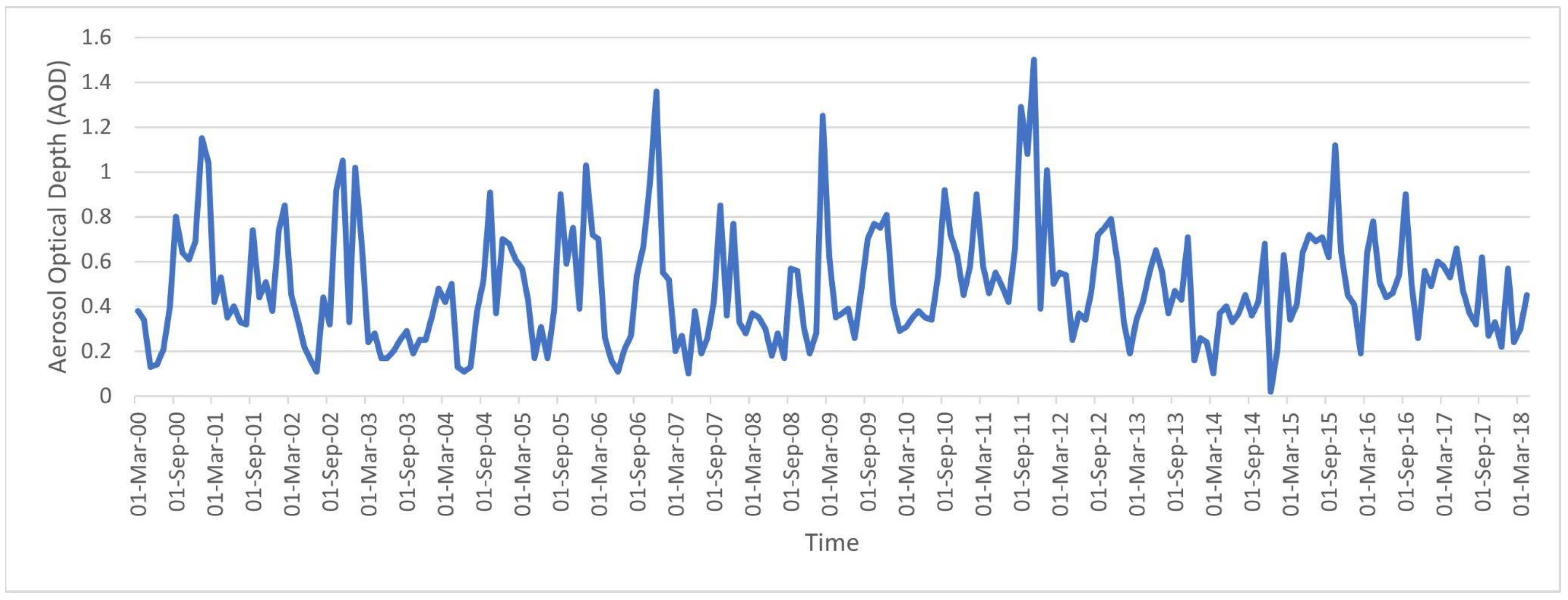
2.5.2. Aerosol Optical Depth

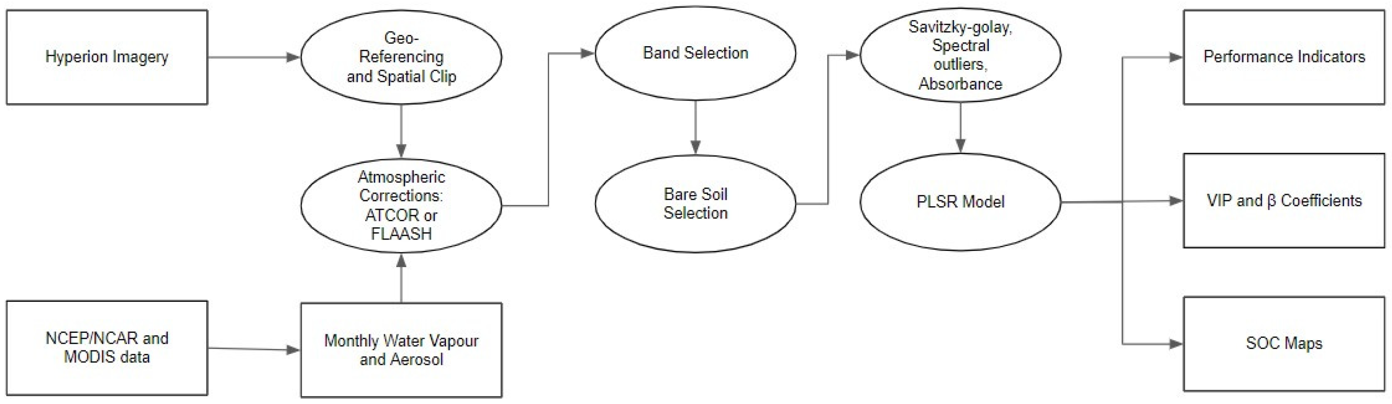
Molecular scattering and absorption can be adequately explained, but not the optical properties of aerosols for the portion of the spectrum dominated by scattering processes rather than thermal emission. Kaufman [45] demonstrated how aerosols reduce apparent spatial resolution, alter the apparent spectral characteristics, resulting in a loss of classification accuracy. From MODIS MOD08_M3 V6, which is an atmosphere global product that contains monthly 1 × 1-degree grid average values of atmospheric parameters, the AOD values over the study area ranged from 0.02 to 1.5 over the last 15 years (from 2000 to 2015, Figure 3, Table 1) [46].

At the date of Hyperion images acquisition, over the study area, the AOD value would be estimated between 0.25 and 0.26. Finally, considering the “Mid Latitude Summer” climatic condition over the study area, the default AOD value in FLAASH would be 1. The Hyperion data were corrected from atmospheric effects using seven AOD values in FLAASH: 0.2, 0.4, 0.6, 0.8, 1, 1.2, and 1.4.

2.6. Methodology

The FLAASH and ATCOR atmospheric correction was performed in ENVI and ATCOR software, respectively. Bands selection and bare soil pixels selection were performed in QGIS, an open-source GIS software. The regression model, including the calibration data preparation, the model building, and the evaluation of the performances were performed in Matlab(R). Historical AOD and WV data were extracted using the Google Earth Engine platform.

2.7. Atmospheric Correction Models

2.7.1. ATCOR Atmospheric Correction Model

ATCOR uses the MODTRAN5 radiative transfer model [24] with the newest high-resolution transmission molecular absorption (HITRAN) database for atmospheric correction. MODTRAN5 is an updated version with greater spectral resolution and supplementary atmospheric gas treatment [47,48]. In the 400–2500 nm range, ATCOR uses a variable wavenumber grid to achieve a constant spectral sample distance of 0.4 nm [24]. In this study, the band model of MODTRAN was used.

For each image, ATCOR assumes a Lambertian surface and requires a sensor type, flight date, solar zenith angle, sensor view geometry, average ground height, and adjacency range. The initial visibility estimate was 30 km. The spectral specifications for the sensor Hyperion are stored in a calibration file called “hyperion 167.cal” provided by ATCOR. There is an atmospheric database, which consists of look-up tables for radiative transfer calculations that span a wide range of weather situations and sun angles. The user has the option of using the standard MODTRAN model for atmosphere and aerosol types to depict the scene, and each image receives its own MODTRAN solution.

In this study, both Hyperion images were corrected from atmospheric effects with the ATCOR model (Figure 4) using the six WV values, preselected by the ATCOR software: 0.4, 1, 2, 2.9, 4, and 5 cm. The default values of other parameters were selected for running the ATCOR model as described in

Table 2. ATCOR parameters.

Parameter	Selected Value
Atmospheric Model	Mid-Latitude Summer
Adjacency correction	No
Aerosol Model	Rural
Visibility	30 km
Region for water vapor retrieval	820 nm
Spectral polishing	No
CO2	390 ppm
Water vapor	Ranges from 0.9 cm to 3.7 cm

. Six atmospherically corrected Hyperion images were created for both sites (site#1 and site#2).

2.7.2. Fast Line-of-Sight Atmospheric Analysis of Spectral Hypercubus (FLAASH) Atmospheric Correction Model

FLAASH is an atmospheric adjustment approach based on physics [49]. It calculates the parameters needed for RT equations using the MODTRAN4 code, which results in surface reflectance. A scaled DISORT (DIScrete Ordinate Radiative Transfer) algorithm is utilized to calculate atmospheric multiple scattering, and the correlated k technique is employed to represent absorption for places with significant absorption effects. FLAASH, with a resolution of 5 cm⁻¹, results in SSD ranging from 0.08 to 3.12 nm depending on wavelength in the 400–2500 nm range.

Hyperspectral sensors, such as HyMAP, AVIRIS, HYDICE, Hyperion, Probe-1, CASI, and AISA, and multispectral sensors, such as HyMAP, AVIRIS, HYDICE, Hyperion, Probe-1, CASI, and AISA), are supported by FLAASH (such as Landsat, SPOT, IRS, and ASTER). Retrieval of water vapor and aerosol are only possible when the image comprises bands with incorrect wavelength locations. A method for extracting an estimated aerosol/haze amount from chosen dark land pixels in the picture is included in the FLAASH model.

In this study, both Hyperion images were corrected from atmospheric effects with the FLAASH model (Figure 4) using the seven AOD values selected based on the Modis MOD08_M3 V6 product (Section 2.5.2): 0.2, 0.4, 0.6, 0.8, 0.1, 0.12, and 0.14. The default values of other parameters were selected for running the FLAASH model as described in Table 3. Seven atmospherically corrected Hyperion images were created for both sites (site#1 and site#2).

Table 3. FLAASH parameters.

Parameter	Selected Value
Atmospheric Model	Mid-Latitude Summer
Adjacency correction	No
Aerosol Model	Rural
Visibility	30 kms
Region for water vapor retrieval	820 nm
Spectral polishing	No
CO2	390 ppm
Aerosol optical depth	Ranges from 0.02 to 0.15

Table 3. FLAASH parameters.

Parameter	Selected Value
Atmospheric Model	Mid-Latitude Summer
Adjacency correction	No
Aerosol Model	Rural
Visibility	30 kms
Region for water vapor retrieval	820 nm
Spectral polishing	No
CO2	390 ppm
Aerosol optical depth	Ranges from 0.02 to 0.15

2.8. Bands Selection

The HYPERION spectral bands with a very low SNR and those located in the atmospheric absorption bands are removed, as previously done by Gomez et al. [12], Lu et al. [50], and Minu et al. [35]. A total of 122 spectral bands, belonging to spectral ranges from 467 to 854 nm, 1063 to 1336 nm, 1548 to 1790 nm, and 1981 to 2355 nm, were finally kept to estimate SOC content from PLSR models. Different degrees of vertical stripping were indicated by visual observation of individual reflectance bands. It was discovered that excluding certain bands from the study was beneficial [50,51]. This is done after FLAASH or ATCOR has applied atmospheric adjustment (Figure 4). Bands surrounding large atmospheric absorption areas (e.g., at the 950, 1400, 1900, and 2500 nm water absorption bands) that appear as over/under-corrected reflectance values were also removed from the reflectance spectrum. After using the FLAASH and ATCOR algorithms, a few bands with negative or zero reflectance values near the 450 nm spectral area that were not actual reflectance values were also removed.

Finally, a total of 122 spectral bands were used in both ATCOR and FLAASH and then used to estimate SOC content from PLSR models. This is in accordance with the bands used by Minu et al. [35]. These 122 spectral bands belong to the spectral ranges from 467 to 854, 1063 to 1336, 1548 to 1790, and 1981 to 2355 nm.

2.9. Bare Soil Pixels Selection

The Normalized Differential Vegetative Index (NDVI) was used to identify and mask green vegetation pixels [52], based on the following equation:

NDVI = (NIR − Red)/(NIR + Red)

(1)

where NIR and Red are the reflectance measured at 834 nm and 661 nm, respectively. Pixels with NDVI values over 0.2 were masked.

The Modified Normalized Difference Water Index (MNDWI) was used to identify and mask water pixels. The MNDWI is calculated for the enhancement of open water features [53], as follows:

MNDWI = (Green − SWIR₁))/(Green + SWIR₁)

(2)

where Green and SWIR₁ are the reflectance measured at 559 nm and 1609 nm, respectively. It also diminishes built-up area features that are often correlated with open water in other indices. Pixels with MNDWI values greater than 0 were masked.

The Normalized Burned Ratio 2 (NBR2) index was used to mask the dry vegetation [54] as follows:

NBR2 = (SWIR₁ − SWIR₂)/(SWIR₁ + SWIR₂)

(3)

where SWIR₁ and SWIR₂ are the reflectance measured at 1609 nm and 2193 nm, respectively. Pixels with an NBR2 value greater than 0.2 were masked [54].

2.10. Regression Model

2.10.1. Data Preparation

Before performing quantitative statistical analysis, a noise reduction was achieved through standard pre-treatments: a Savitzky–Golay filter with third-order polynomial smoothing and window widths of 61 nm [55], mean centering and variance scaling. A generalised moving average filter, the Savitzky Golay filter [55], is also known as a digital smoothing polynomial filter or least-squares smoothing filter. The filter coefficients are calculated by fitting a polynomial of a particular degree with an unweighted linear least-squares fit. It requires equidistant bandwidth and fits a local polynomial regression on the signal. It is feasible to get a high amount of smoothing without attenuating data features using a higher degree polynomial. Mathematically, it’s nothing more than a weighted sum of nearby values. The Hyperion spectra were filtered with a third order Savitzky Golay filter.

$${\overline{x}}_i=\frac{{{\displaystyle \sum }}_{j=1}^{n}Xij}{n}$$

(4)

Standard normal variate (SNV) calculates the standard deviation of all the pooled variables for the given sample [56]. The entire sample is then normalized by this value, thus giving the sample a unit standard deviation (s = 1).

$$w_i=\sqrt{\frac{{{\displaystyle \sum }}_{j=1}^n\left(Xij-{\overline{x}}_i\right)2}{n-1}}+{\delta }^{-1}$$

(5)

where n is the number of variables, x_ij is the value of the jth variable for the ith sample, and δ is a user-definable offset. The user-definable offset can be used to avoid over-normalizing samples which have near-zero standard deviation. The default value for this offset is zero, indicating that samples will be normalized by their unweighted standard deviation. The selection of δ is dependent on the scale of the variables. A setting near the expected noise level (in the variables’ units) is a good approximation.

Outliers are observations that differ significantly from normal values and are not compatible with the rest of the data [57,58]. Spectra can be defined as a spectral outlier when the sample is spectrally different from the rest of the samples. Out of the 98 samples for which SOC values are present, spectral outliers were identified using Mahalanobis distance [59]. This class of methods only uses distance space to flag outlier observations. The Mahalanobis distance (MD) for the ith observation is given by:

$$\begin{gathered} M{D}_i=\sqrt{\left(x_i-\overline{x}\right)t{C}^{-1 }\left(x_i-\overline{x}\right)} \\ C=\frac{1}{n-1}{X}^{\prime }X \end{gathered}$$

(6)

where X is the data matrix of size n × p, where p is the number of variables and n is the number of observations. xᵢ is an observation (a row of X), $\overline{x}$ is the mean vector, and C is the sample covariance matrix which gives information about the covariance structure of the data. In the analysis, Mahalanobis distance cutoff was set to 3.

2.10.2. PLSR with Leave-One-Out Cross-Validation (LOOCV)

In this study, Partial Least Squares Regression (PLSR) is carried out to find predictive models for soil organic carbon data and discusses the effectiveness of these methods in predicting soil carbon using spaceborne Hyperspectral data. Here, the PLSR method is used to regress a relationship between response variables to many predictor variables [60]. Care should be taken whilst choosing the number of latent variables. Using many components will lead to a good fitting model but is a strategy that leads to overfitting. In this case, cross-validation, which is a widely used method, was used in choosing the optimal number of variables. The maximum number of latent variables was defined as 10, then the optimal number of latent variables was determined using the prediction residual error sum of squares (PRESS) analysis. This allows avoiding under- and over-fitting.

Cross validations also avoid overfitting by not using the same data to both fit a model and to estimate prediction error. In this study, 10-fold cross-validation was used. Here the original data was divided into subsets or folds, which in this case is 10. One of the folds is not used in the model building and is used to estimate the error. This process is replicated for all the folds for multiple iterations. This leads to a minimized prediction error for different numbers of latent variables. Hence there is no fixed validation dataset.

2.10.3. Model Evaluation

The coefficient of determination (R²_cv) is the percent of the total variation in the response variable that is explained by the regression line [61]. The R²_cv was obtained for the cross-validation dataset as follows:

$$R^2=1-\frac{SSE}{SST}$$

(7)

where SSE is the sum squared differences between the predicted and observed value, and SST is the sum of squared differences between the observed and overall mean value.

The root means squared error (RMSE_cv) is the average prediction error (square root of mean squared error) [62].

$$RMSE=\sqrt{\frac{{{\displaystyle \sum }}_{i=1}^n(y_i-{\widehat{y}}_i)2}{n}}$$

(8)

RPD is the ratio of the standard deviation (SD) of analyzed data to RMSE_cv. It is given by the following equation:

$$RPD=\frac{SD}{RMSE}$$

(9)

Chang and Laird [63] defined three classes of RPD: category A (RPD > 2) describes models that can accurately predict the soil property, category B (2 > RPD > 1.4) describes models with limited predictive power, and category C (RPD < 1.4) describes models that have no prediction ability.

The ratio of performance to interquartile (RPIQ) value is more objective than RPD [64] as it is based on quartiles, which better represents the spread of the population. The quartiles are milestones in the population range: Q1 is the value below which 25% of the samples are found; Q3 is the value below which 75% of the samples are found; and Q2, commonly called the median, is the value under which 50% of samples are found. RPIQ is the ratio of IQ to RMSE, where IQ is the difference between the third quartile Q3 and the first quartile Q1. A larger RPIQ value indicates improved model performance. The formula is shown as follows:

$$\begin{gathered} IQ=Q3-Q1 \\ RPIQ=\frac{IQ}{RMSE} \end{gathered}$$

(10)

The Variable Importance in Projections (VIP) is a weighted sum of squares of PLS weights, with weights generated from each PLS component’s Y-Variance [65,66]. Multiplying the VIP and the absolute value of PLS regression coefficients from the PLSR model yields the wavelengths important for modeling. Each PLSR model was examined for a higher value for the product of absolute regression coefficient and variable importance for projection (VIP) to identify significant wavelengths in determining SOC content from spectral reflectance data rather than the full spectrum.

2.10.4. SOC Mapping

The calibrated PLSR models were applied to bare soil pixels. This would produce an estimated SOC map for each model. In case of a negative estimated SOC value, this value was replaced by 0 g/kg. So, a total of 13 SOC maps were obtained: six from the Hyperion images corrected by FLAASH and different AOD values and seven from the Hyperion images corrected by ATCOR and different WV values. A map of the standard deviation of the estimated SOC along the six SOC maps obtained from the Hyperion images corrected by FLAASH was produced. A map of the standard deviation of the estimated SOC along the seven SOC maps obtained from the Hyperion images corrected by ATCOR was produced.

3. Results

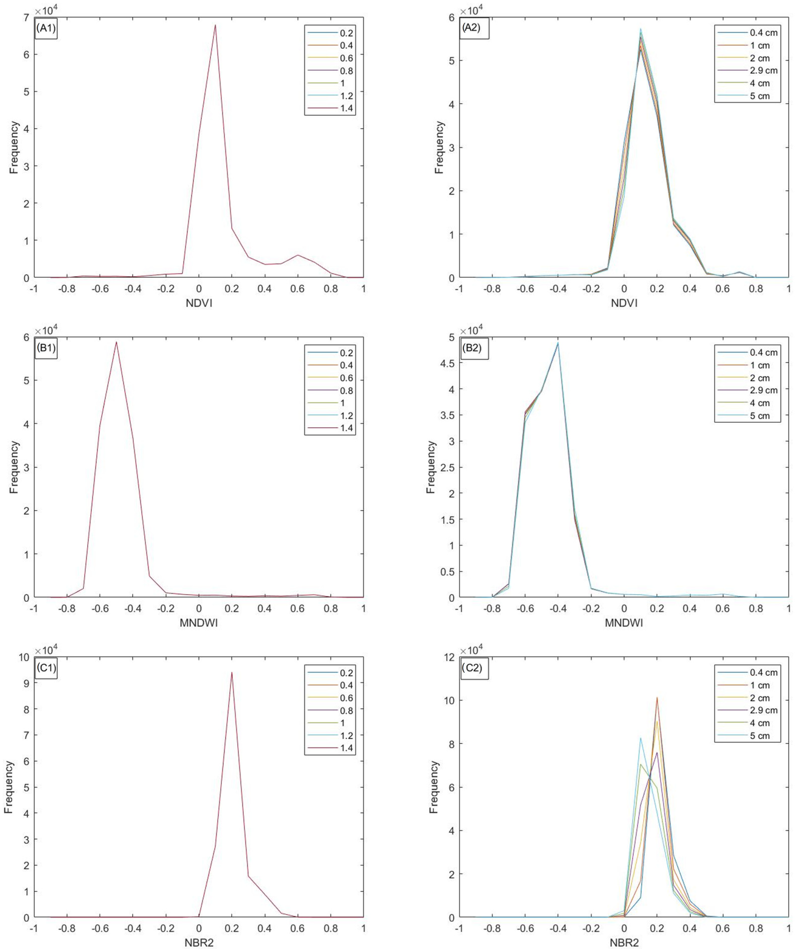
3.1. Bare Soil Coverage Analysis

Similar histograms of NDVI, MNDWI and NBR2 values were obtained whatever be the AOD value used in the FLAASH model to correct the Hyperion images (Figure 5(A1,B1,C1)). Moreover, a similar bare soil coverage of 82.35% was obtained, whatever be the used AOD value (

Table 4. Figures of merit obtained from PLSR models, based on Hyperion data corrected by the FLAASH method, and depending on 7 values of AOD.

AOD	0.2	0.4	0.6	0.8	1	1.2	1.4
Bare soil coverage (%)	82.35	82.35	82.35	82.35	82.35	82.35	82.35
R2cv	0.79	0.79	0.79	0.79	0.79	0.79	0.79
RMSEcv (%)	0.40	0.41	0.40	0.40	0.40	0.40	0.40
RPD	2.23	2.21	2.22	2.23	2.23	2.23	2.23
RPIQ	3.26	3.24	3.25	3.26	3.27	3.26	3.26
bias (%)	0.32	0.33	0.33	0.33	0.33	0.33	0.33
Number of Latent Variables	2	2	2	2	4	2	2

). So, a variation of the AOD value used in the FLAASH model did not impact the reflectance at the spectral bands used to calculate the NDVI, MNDWI, and NBR2 spectral indexes (Equations (1)–(3)).

By contrast, the selection of the WV value used in the ATCOR model to correct the Hyperion images appeared to impact marginally the spectral bands used to calculate the NDVI, MNDWI, and NBR2 spectral indexes (Equations (1)–(3)). Histograms of NDVI and MNDWI values displayed the same shapes irrespective of the WV value used in the ATCOR model, with the same modes at 0.1 and −0.4 for NDVI and MNDWI, respectively (Figure 5(A2,B2)). Histograms of NBR2 values displayed the same shapes with a slight shift of modes (Figure 5(C2)). Consequently, the bare soil coverage varied depending on the used WV value from 75 % (obtained with a WV of 0.4) to 84 % (obtained with a WV of 2) (

Table 5. Figures of merit obtained from PLSR models, based on Hyperion data corrected by the ATCOR method, and depending on 6 values of WV. The best performances are highlighted in bold.

Water Vapor (in cm)	0.4	1	2	2.9	4	5
Bare soil coverage (%)	75.04	80.54	84.04	83.50	83.17	82.85
R2cv	0.75	0.78	0.79	0.75	0.72	0.72
RMSEcv (%)	0.44	0.41	0.41	0.44	0.47	0.46
RPD	2.04	2.17	2.19	2.03	1.91	1.93
RPIQ	2.98	3.17	3.21	2.97	2.80	2.83
bias (%)	0.35	0.33	0.31	0.34	0.38	0.35
Number of Latent Variables	5	2	3	4	2	6

).

For the same pixel, it is observed that there is no variation of the spectrum along with the AOD range, but variations can be observed of the spectrum along with the WV range (Figure 6). No absorption bands of clay or carbonate are observed in the spectrum with FLAASH AC. Meanwhile, for the spectrum with ATCOR AC, the higher the WV the higher the albedo of the spectra.

3.2. SOC Prediction Models Performances Using Hyperion Data Corrected by FLAASH

A PLSR model was built from the Hyperion spectra corrected by the FLAASH model and from SOC associated with the available soil samples. Four spectral outliers were removed from the calibration database, regardless of the study area, and the number of latent variables were determined following the rule of the first local minimum of the RMSE_cv and varied between 2 and 4 (Table 4). The performance of the PLSR models was correct, with R²_cv of 0.79, RMSE_cv of 0.40 and RPD of 2.2 whatever be the AOD values (Table 4). So, the selection of the AOD for correcting the Hyperion images using the FLAASH model did not affect the model’s performance for SOC prediction.

3.3. SOC Prediction Models Performances Using Hyperion Data Corrected by ATCOR

A PLSR model was built from the Hyperion spectra corrected by the ATCOR model and from SOC associated with the available soil samples. Four spectral outliers were removed from the calibration database, regardless of the study area, and the number of latent variables were determined following the rule of the first local minimum of the RMSE_cv, which varied between 2 and 6 (Table 5). The performances of the PLSR models were correct, with R²_cv from 0.72 to 0.79, RMSE_cv from 0.41 to 0.47 and RPD from 1.9 to 2.2 (Table 5).

The best performance was obtained from the model based on spectra corrected by the ATCOR model and WV of 2 cm (Table 5). The lowest performance was obtained from the model based on spectra corrected by the ATCOR model and WV of 4 cm (Table 5).

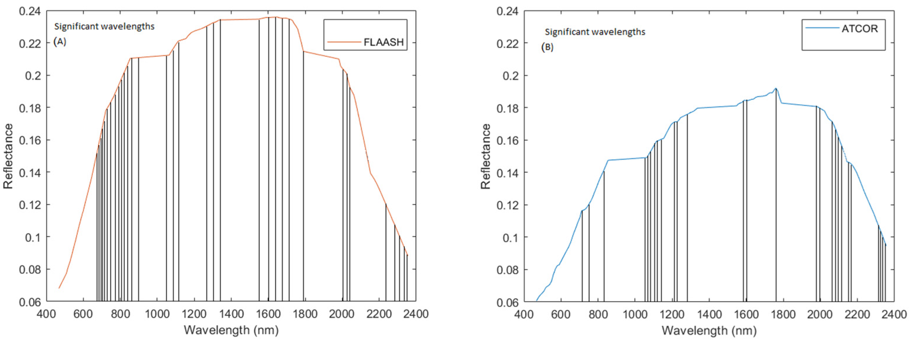
3.4. Significant Wavelengths for SOC Estimation

Between 41 to 43 wavelengths were identified as significant in the PLSR models built from the 6 Hyperion images corrected by FLAASH and different AOD values. 41 of these significant wavelengths are common between the six PLSR models. 48% of the significant wavelengths belonged to the VNIR (400–1100 nm) and 42% of the significant wavelengths belonged to the spectral domain from 1100–2000 nm (Figure 7A). In the region, 2000–2400 nm fewer significant wavelengths (14%) were found corresponding to some minerals (Carbonates and Clay) (Figure 7A).

Between 28 to 42 wavelengths were identified as significant in the PLSR models built from the two Hyperion images corrected by ATCOR and different WV values, and only 1 of these significant wavelengths are common between the thirteen PLSR models. Most of the significant wavelengths (36%) belonged to the spectral domain from 1100 to 2000 nm (Figure 7B). 33% of significant wavelengths belonged to the spectral domain from 2000–2500 nm (Figure 7B).

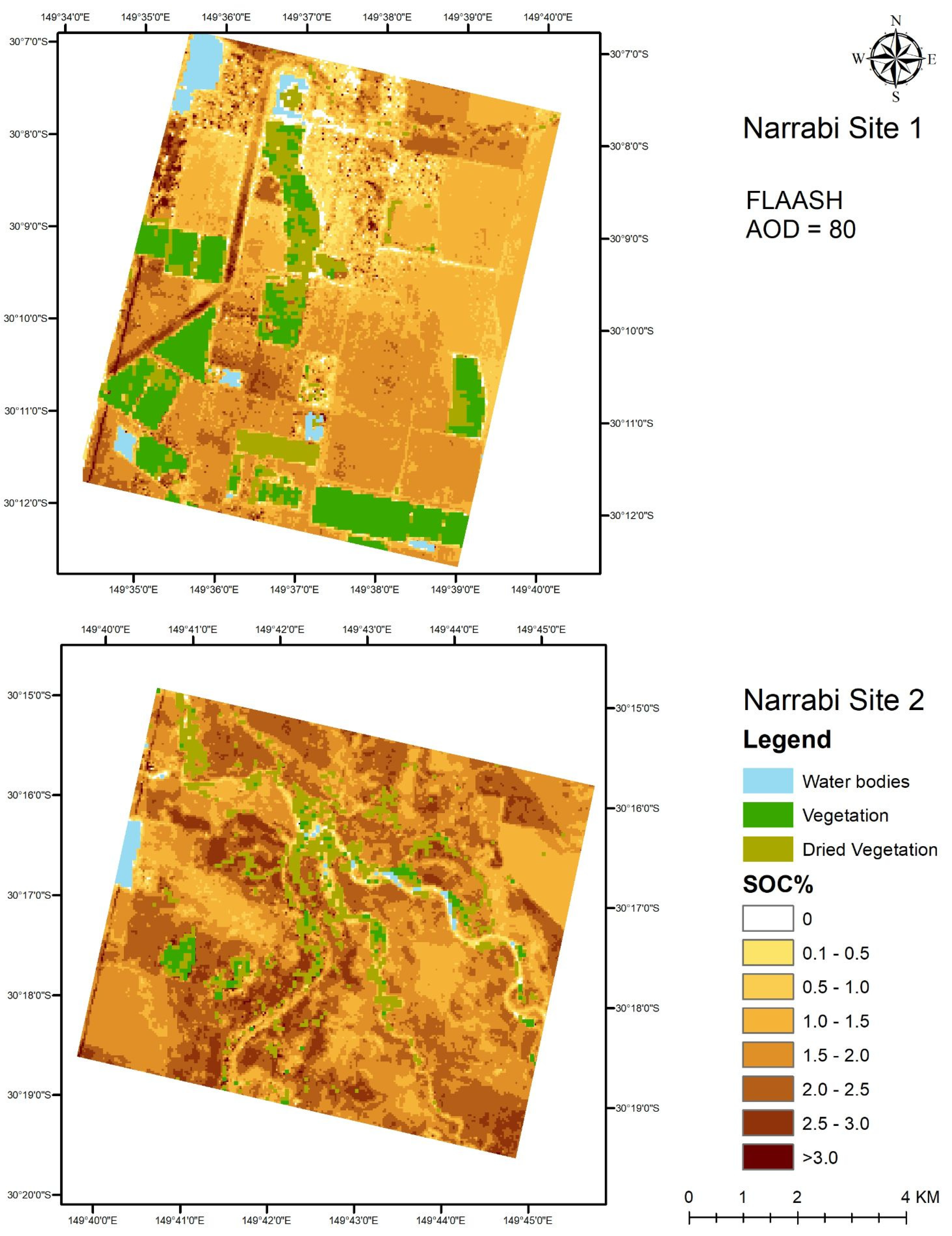
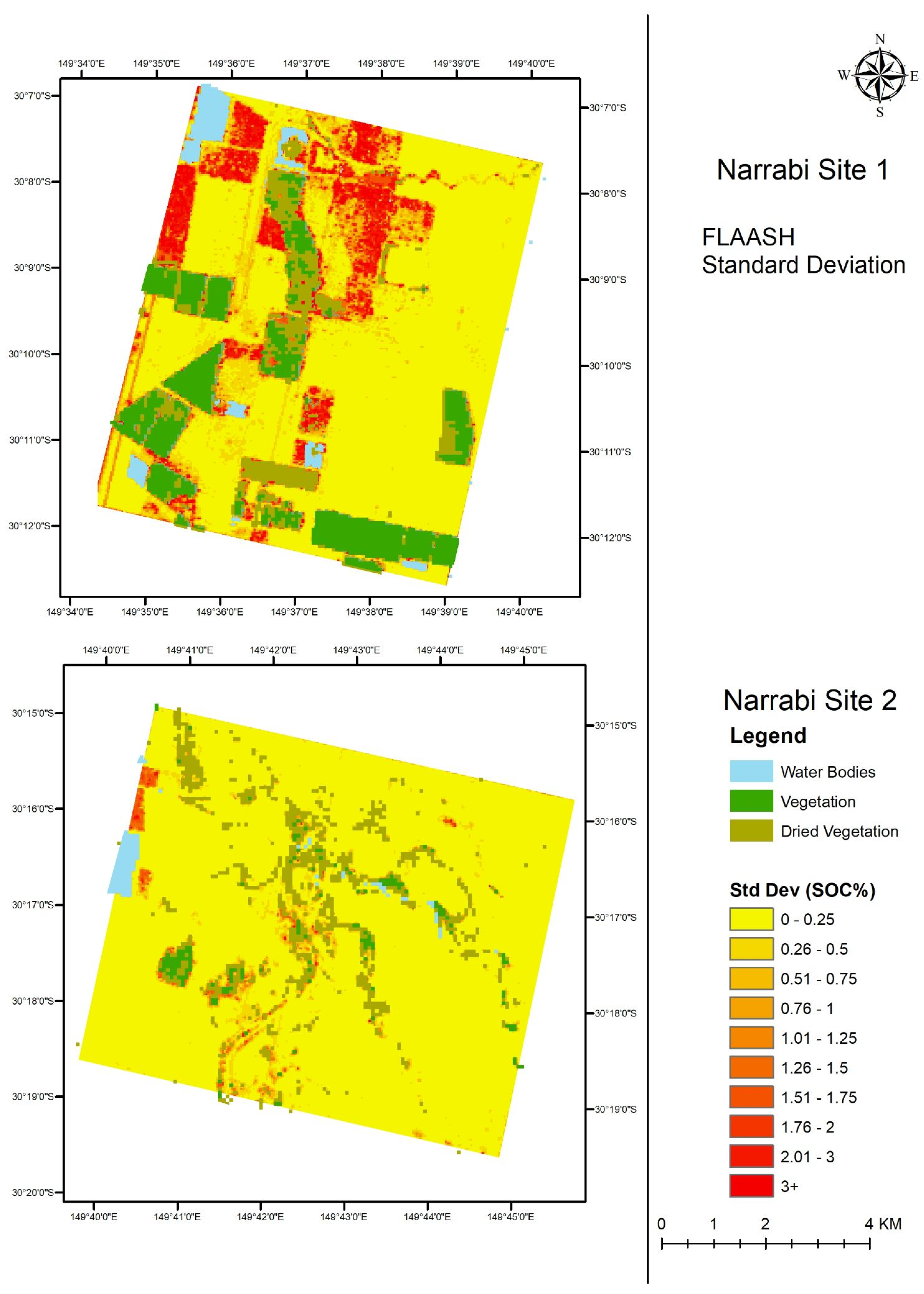
3.5. SOC Maps Using Hyperion Data Corrected by FLAASH

PLSR models built from Hyperion images corrected with different AOD values using the FLAASH model were applied to the bare soil pixels to produce SOC maps over both sites. The percentage of negative predictive SOC values over both sites varied from 2.64 to 6.31% depending on the AOD value used to correct the Hyperion images with the FLAASH model (

Table 6. Percentage of negative SOC estimated using Hyperion data corrected by FLAASH, from both the sites.

AOD	Negative SOC Pixels %
0.2	6.31
0.4	1.93
0.6	2.64
0.8	2.65
1.0	3.27
1.2	4.98
1.4	5.50

). The percentage of negative predictive SOC increases from an AOD of 0.4 to AOD 1.4 (Table 6) while the highest percentage was observed with an AOD of 0.2 (Table 6).

The distributions of SOC contents estimated by PLSR over both sites varied slightly when using an AOD value from 0.4 to 1.4 with a mode around 1.8%, while the distribution of SOC contents estimated by PLSR when using an AOD value of 0.2 has a mode around 1.6% (Figure 8). The SOC map using AOD 0.2 has a greater number of pixels which have SOC of greater than 3%. This is not observed in the other SOC maps. The SOC prediction map with AOD 80 is visualized in the Figure 9.

Variation in the SOC content of the pixels adjacent and in between vegetation pixels can also be observed. This can be clearly seen in the Standard Deviation map (Figure 10). A higher standard deviation along the riverbed in site#2 is observed. This may be due to no bare soil and a mixture of water, green, and dry vegetation. High standard deviation is observed in areas that have negative values with AOD = 0.2 and AOD > 1.0.

It is observed that there is a slight deviation in the spectral signatures with varying AOD in the VNIR region of 400 to 1100 nm and no deviation in the rest of the spectrum up to 2400 nm (Figure 6). The percentage of bare soil pixel is very consistent 82.35% and good consistency is observed for the significant wavelengths for the prediction model with FLAASH atmospheric correction (Table 4). Hence due to these observations, consistency can be observed in the model performance across varying AOD levels.

The range of AOD in the Narrabri region varies from 0.02 to 1.5 as per Table 1. Comparing the SOC maps obtained by varying the AOD level with the exception of AOD level 0.2, good consistency prediction from AOD 0.4 to AOD 1.4 is observed. This is also confirmed by the histogram as per (Figure 8). The standard deviation map of SOC variation is fairly consistent with high variation at a few places. These places match with farm boundaries indicating inconsistencies at a farm level.

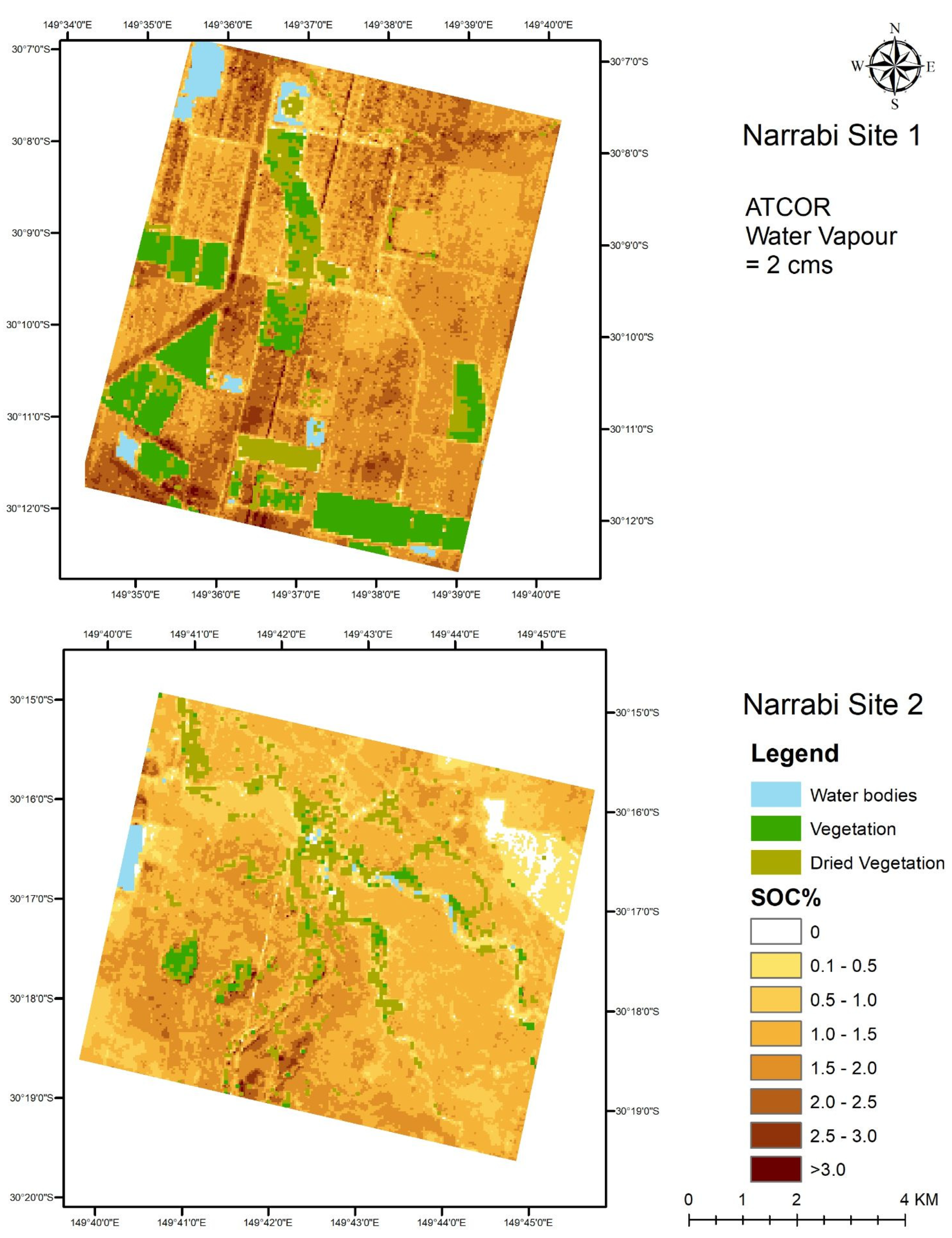
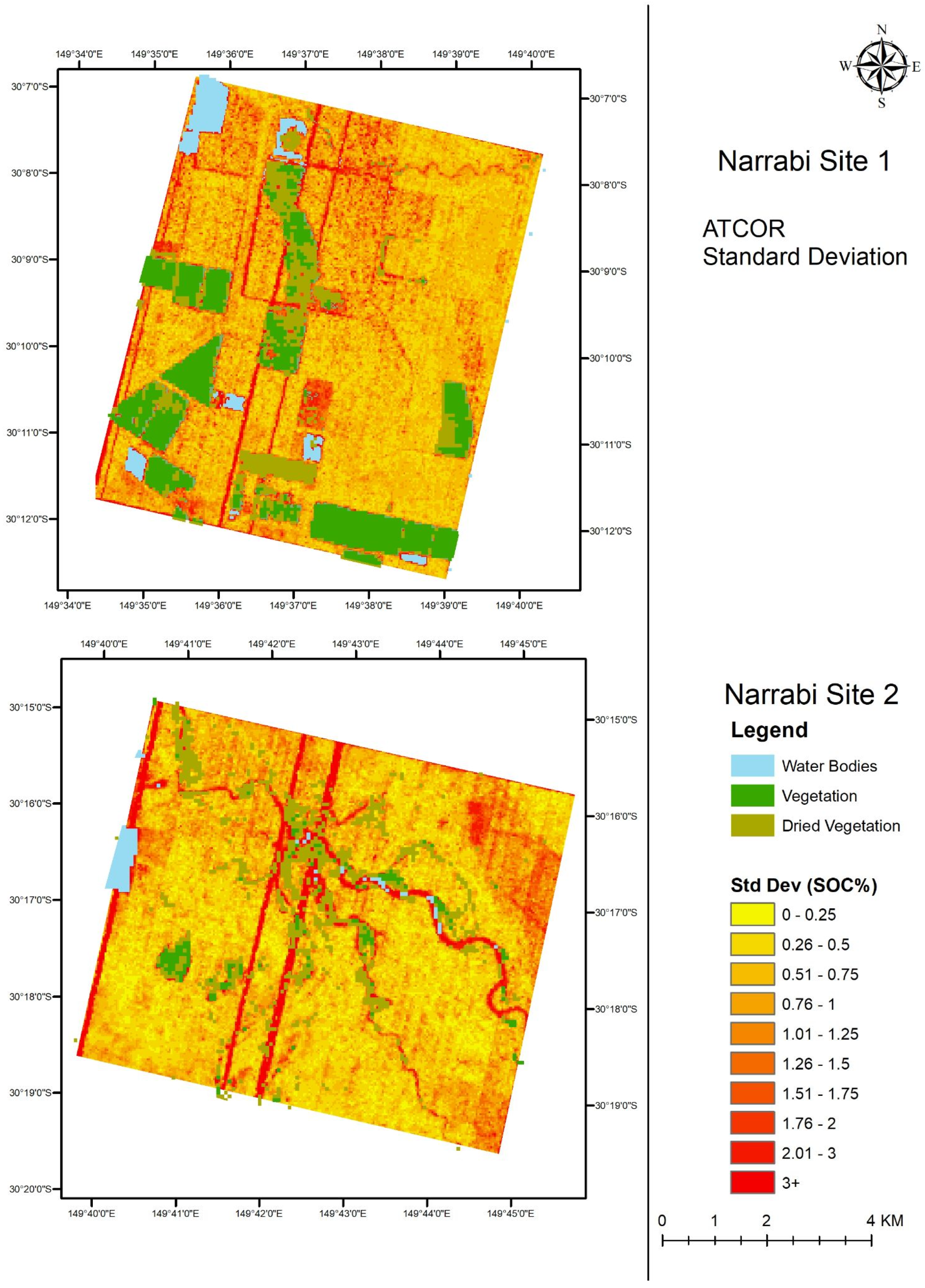
3.6. SOC Maps Using Hyperion Data Corrected by ATCOR

PLSR models built from Hyperion images corrected with different WV values using the ATCOR model were applied to the bare soil pixels to produce SOC maps over both sites.

The percentage of negative predictive SOC values over both areas varied from 1.78% (obtained with a WV of 5 cm) to 5.51% (obtained with a WV of 0.4 cm) depending on the WV value used to correct the Hyperion images with the ATCOR model (

Table 7. Percentage of negative SOC estimated using Hyperion data corrected by ATCOR, from both the sites.

Water Vapor (in cms)	Negative SOC Pixels %
0.4	5.51
1.0	4.60
2.0	4.63
2.9	3.22
4.0	4.53
5.0	1.78

).

The distributions of SOC contents estimated by PLSR over both sites varied significantly when using a WV value from 0.4 to 5 cm (Figure 11), with different modes from 1.2% (obtained with a WV of 2 cm) to 1.8% of SOC (obtained with a WV of 0.4 cm). The PLSR model built from Hyperion spectra corrected by ATCOR and a WV value of 2 cm provided the best performances (Table 5) while the estimated SOC contents over the sites displayed the lower SOC values (Figure 11). The SOC prediction map with WV 2 cm is visualized in the Figure 12.

There is variation in the SOC map using WV of 0.4, 4, and 5 cm, respectively (Figure 11), compared to the rest of the maps, which are fairly consistent. Variation in the pixels around and between vegetation can also be observed. This can be clearly seen in the standard deviation map (Figure 13). High standard deviation is observed along the riverbed due to no bare soil pixel and the mixture of water and vegetation pixels in site#2. A couple of prominent stripes in site#1 and site#2 are observed. In site#1, high standard deviations are observed along the farm boundaries.

The distribution of SOC estimates varied with different WV conditions though similarity in the modes is observed between 1 cm, 2 cm, and 2.9 cm (Figure 11). The best results statistically are obtained for the models in this range. A higher percentage of SOC is estimated in the 0.4 cm, 4 cm, and 5 cm (Figure 11). It is to be noted these ranges are not in the range of WV over the study area (Figure 2, extracted from NCEP). Small deviations in SOC can be observed throughout the study area and stronger deviations in SOC can be observed where there is uncertainty associated with surface types like riverbeds and boundaries of farm plot (Figure 13).

4. Discussions

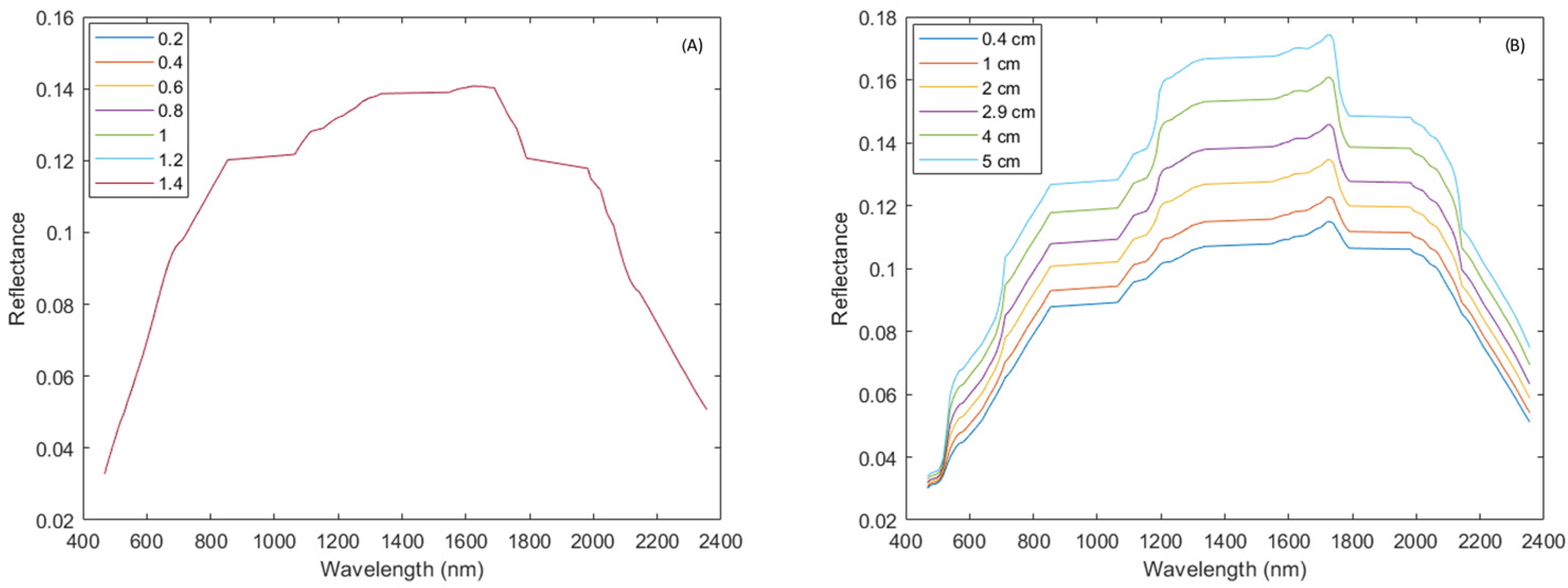
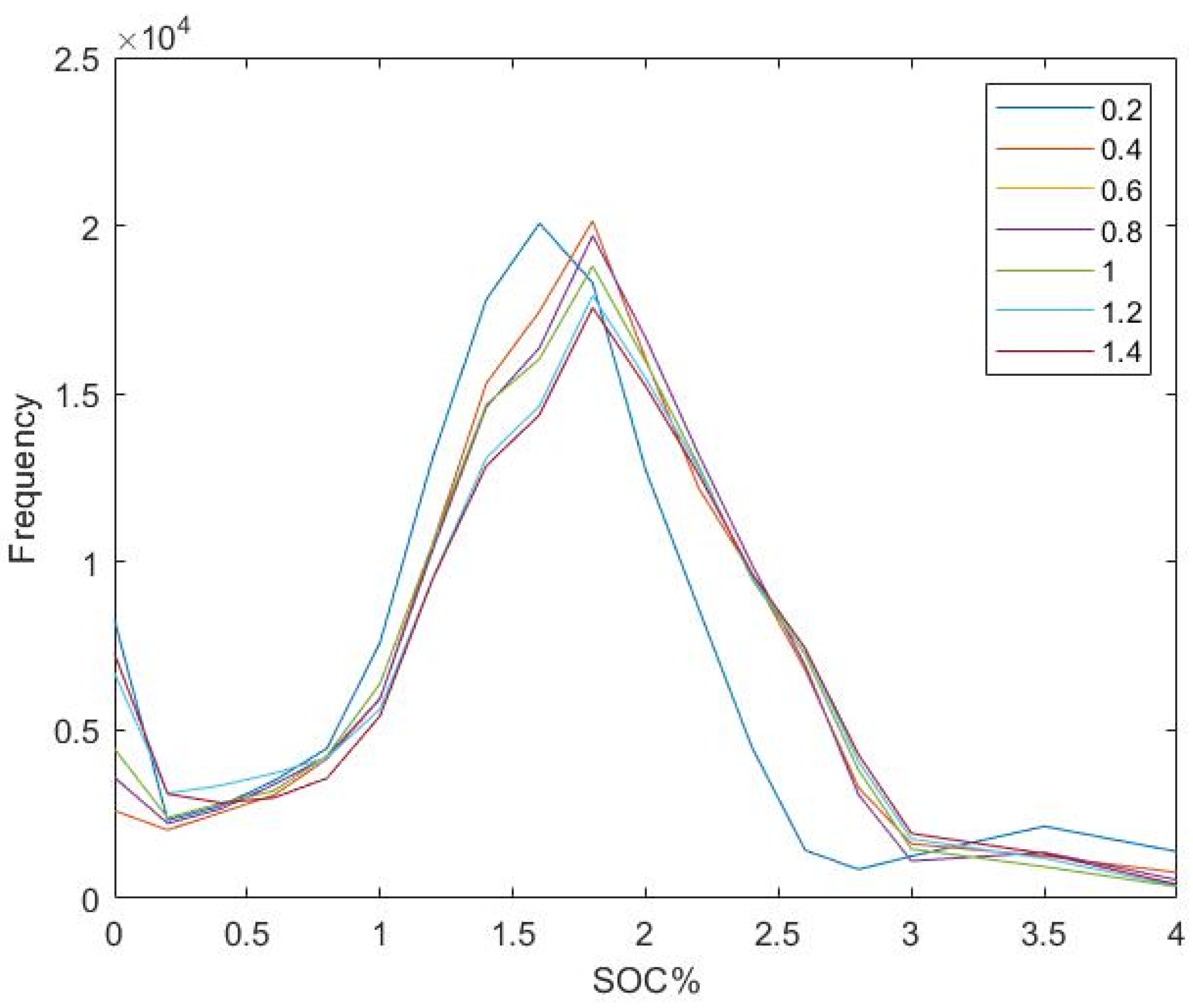
4.1. Bare Soil Identification Variations Based on Atmospheric Parameters

The choice of the AOD parameter in the FLAASH AC method seems to have no impact on the three tested spectral indexes (NDVI, MNDWI, and NBR2; Figure 5(A1,B1,C1)). Therefore, the percentage of bare soil pixels, based on NDVI indexes, remained constant along the AOD parameters in FLAASH (Table 4). On the other hand, the WV parameter in the ATCOR AC method affects the three tested spectral indexes (NDVI, MNDWI, and NBR2; Figure 5(A2,B2,C2)). Therefore, the percentage of bare soil pixels identification varied depending on the WV parameter (Table 5).

As soil properties estimations are affected by the presence of green and dry vegetation on spectra [16,17], bare soil pixel identification is a major step in soil properties mapping by remote sensing. As this step of bare soil pixels identification depends on spectral indices calculations (e.g., NDVI and NBR2) [67,68], the choice of the AOD parameter may impact the soil properties mapping. Additionally, the topsoil moisture conditions may also affect reflectance spectra and therefore spectral indices calculation, such as the NBR2 index [67], and then soil properties mapping [18].

4.2. Performance Analysis of PLSR Models after FLAASH AC Method

The SOC predictions obtained by PLSR models using Hyperion data corrected by the FLAASH AC method were accurate within the range of the AOD parameter (Table 4 and Table 5). These PLSR performances are in accordance with Gomez et al. [12] using the same data and the Atmospheric Removal Program’ (ATREM) model, and with Minu et.al [35] using the same data and the FLAASH method, who obtained R²_cv of 0.71 and RMSE_cv of 0.46% for SOC prediction. These PLSR performances for mapping SOC are slightly better than those obtained by Lu et al. [50], who also used the FLAASH AC method to derive reflectance from Hyperion radiance.

The performance results in the SOC prediction model using Hyperion data corrected by the FLAASH method show a constant R²_cv and RMSE_cv of 0.79 and 0.4% whatever the AOD parameter. This is in line with the study of Griffin et al. [39] where for the dry and relatively clear rural aerosol case, the effect of varying the aerosol optical depth produces errors < 0.02 with sensitivity. Davaadorj A. [40] also stated that FLAASH produced less variability in reflectance with varying AOD compared to other AC models (ATCOR). Most of the significant wavelengths (48%, Figure 7A) used in the PLSR models belonged to the VNIR spectral range (400–1100 nm) and more precisely around 600 to 750 nm which has been also referred by Ben Dor et al. [69] confirming that PLSR models are based on spectral features. The remaining 42% of significant wavelengths belonged to the spectral domain from 1100–2000 nm (Figure 7), including 1358 nm, probably due to OH ions in water [70].

The distribution of SOC estimation over bare soils were similar with Hyperion images corrected with FLAASH and AOD of 0.4 to 1.4 (Figure 8). While constant PLSR performances were observed whatever the AOD parameters (Table 4), differences in the SOC mapping can be observed in the maps (Figure 10). The differences in SOC estimations over some fields (Figure 10) due to the choice of AOD in FLAASH may be due to dry vegetation residue [71]. Studies by Nazeer et al. [41] and Bassani et al. [42] showed that influences of AOD vary with respect to the surface types, such as grass, water, artificial turf, sand etc. The current study deals with only one surface type i.e., bare soil, whereas compared to Nazeer et al. [41] and Bassani et al. [42] who accounted for multiple surface types.

4.3. Performance Analysis of PLSR Models after ATCOR AC Method

The SOC predictions obtained by PLSR models after the ATCOR AC method were accurate within the range of the WV (Table 5). These PLSR performances are in accordance with Gomez et al. [12] using ATREM AC method [20,72] and with Minu et.al [35] using the same data and the ATCOR AC method and obtained R²_cv of 0.76, respectively.

In the ATCOR method, the R²_cv lies in between 0.72 and 0.79 and variations in RPD and RPIQ values can be observed. A RPD higher than 2 is observed for WV of 0.4 to 2.9 cm while RPD values in between 1.91 to 2 were observed for WV 4 to 5 cm. An increase in the reflectance values of the spectral signatures for higher values of WV i.e., 4 cm, and 5 cm in the VNIR region of 400–1100 nm, as well as SWIR region of 1200 to 2400 nm (Figure 6B), is observed. Consistency in the significant wavelengths of the models using 1, 2, and 2.9 cm of WV is seen. 33% of significant bands in predicting SOC are in the region 2000–2400 nm (Figure 7). Henderson et al. [8] showed that soils generated from various parent materials had the best correlation with SOC concentration at wavelengths of 1955–1965, 2215, 2265, 2285–2295, and 2315–2495 nm. A combination of metal–OH bonding and O–H stretching causes an absorption band in the soil signature (Figure 6B) around 2200 nm [73]. In an ATCOR adjusted signal, this absorption band is retrieved. At wavelengths between 640 and 690 nm, Bartholomeus et al. [16] highlighted the strongest association between the inverse of reflectance and SOC (Figure 6B). They also discovered a negative relationship with respect to SOC between the area of the absorption feature between 2050 and 2200 nm.

Best SOC estimation performances were obtained with Hyperion images corrected with ATCOR and WV of 2 cm (Table 5), which is the default parameter in for “Mid-latitude summer” context (Table 3, [24]), while at the date of Hyperion images acquisition, the WV value would be estimated between 2.8 cm and 3.1 cm (Figure 2, extracted from NCEP). Inversely, worst SOC estimation performances were obtained with Hyperion images corrected with ATCOR and WV of 4 and 5 cm (Table 5) which are not in the range of WV over the study area from NCEP data (Figure 2).

4.4. ATCOR versus FLAASH for SOC Predictions

The best SOC prediction model after the ATCOR method was obtained with a WV of 2 cm (Table 5) and gave similar performance than the one after FLAASH method and whatever the AOD. Though the overall percentage of the bare soil pixel selection using spectral indices between ATCOR method and FLAASH method was similar (Table 4 and Table 5), FLAASH method showed more consistency than the ATCOR method. The study conducted by Yusuf et al. 2018 [74] showed that for rural aerosol model FLAASH and ATCOR showed similar Standard Error of Estimate for surface types such as vegetation, sand, and water bodies. In the study conducted by Marcello et al. [75] on soil using worldview imagery using for a rural aerosol model, FLAASH gave an RMSE of 0.0398 and ATCOR gave an RMSE of 0.0406, which is line with the superior RMSE of FLAASH over ATCOR (Table 4 and Table 5).

The reflectance obtained by FLAASH spectra has a slightly higher albedo compared to ATCOR spectra (Figure 6). Similar results have been also observed by Manakos et al. [76] where FLAASH and ATCOR spectra of rural aerosol model were studied with respect to Asphalt and Gravel surface types. The comparison of Spectral angle mapper results for FLAASH and ATCOR were similar for the Asphalt surface type, but FLAASH performed slightly better with the Gravel surface type [76]. Majority of the significant wavelengths were found after 2000 nm in the ATCOR method (Figure 7B), whereas the majority of the significant wavelengths were found in the visible region in the FLAASH method (Figure 7A). Similar results were arrived at by Minu et al. [35] while comparing FLAASH and ATCOR for the soil reflectance. FLAASH method showed better consistency overall in the SOC distribution than the ATCOR method (Figure 8 and Figure 11). With respect to mapping of SOC, FLAASH method showed high standard deviations at a few farms whereas salt and pepper standard deviation distribution was found throughout the study area (Figure 10 and Figure 13).

5. Conclusions

This study highlights the influence of AOD and WV input parameters in AC methods. The AOD parameter was found to have no impact on performance of the FLAASH method and the spectral reflectance. Some amount of variability of estimated SOC was found at low values of AOD i.e., 0.2 and it was found to be fairly consistent at other values of AOD. Variation of the WV had an effect on the performance of the ATCOR method. The best performance of the ATCOR method was observed at 2 cm. With increase in WV, there was increase in the reflectance values between 1000 nm and 2000 nm. The estimation of SOC was consistent around the default value of 2 cm (i.e., from 1 cm to 2.9 cm) but inconsistency is observed at WV < 1 cm and >2.9 cm. Hence in terms of atmospheric parameters, it is found that AOD is a more robust parameter to WV in terms of uncertainty in selection. Caution must be exercised when selecting values of WV in ATCOR method which are not close to the default parameter. As Hyperion is a moderate resolution satellite of 30 m spatial resolution, the bare soil pixel selection is an important step. Wrong bare soil classification especially at the locations when different surface types meet has a high impact and uncertainty on the estimated SOC.

Finally, the next hyperspectral sensors (EnMAP, PRISMA, and HyspIRI) will generate an increasing amount of VNIR/SWIR data around the planet, providing a new chance for mapping topsoil features. If the soil spectroscopy community tries to produce frequently topsoil characteristics maps, the selection of a robust and appropriate AC method, input AC parameters, regression method, and bare soil identification process will become crucial phases.

References

1. Lal, R. Soil health and carbon management. Food Energy Secur. 2016, 5, 212–222. [Google Scholar] [CrossRef]
2. Xiao, J.; Chevallier, F.; Gomez, C.; Guanter, L.; Hicke, J.A.; Huete, A.R.; Ichii, K.; Ni, W.; Pang, Y.; Rahman, A.F.; et al. Remote sensing of the terrestrial carbon cycle: A review of advances over 50 years. Remote Sens. Environ. 2019, 233, 111383. [Google Scholar] [CrossRef]
3. Sanchez, P.A.; Ahamed, S.; Carré, F.; Hartemink, A.E.; Hempel, J.; Huising, J.; Lagacherie, P.; McBratney, A.B.; McKenzie, N.J.; de Lourdes Mendonça-Santos, M.; et al. Digital soil map of the world. Science 2009, 325, 680–681. [Google Scholar] [CrossRef] [PubMed] [Green Version]
4. Zaehle, S. Terrestrial nitrogen–carbon cycle interactions at the global scale. Philos. Trans. R. Soc. B Biol. Sci. 2013, 368, 20130125. [Google Scholar] [CrossRef] [Green Version]
5. Gholizadeh, A.; Borůvka, L.; Saberioon, M.; Vašát, R. Visible, near infrared, and mid-infrared spectroscopy applications for soil assessment with emphasis on soil organic matter content and quality: State-of-the-art and key issues. Appl. Spectrosc. 2013, 67, 1349–1362. [Google Scholar] [CrossRef]
6. Chang, C.W.; Laird, D.A. Near-infrared reflectance spectroscopic analysis of soil C and N. Soil Sci. 2002, 167, 110–116. [Google Scholar] [CrossRef]
7. Beyer, L.; Kahle, P.; Kretschmer, H.; Wu, Q. Soil organic matter composition of man-impacted urban sites in North Germany. J. Plant Nutr. Soil Sci. 2001, 164, 359–364. [Google Scholar] [CrossRef]
8. Henderson, T.L.; Baumgardner, M.F.; Franzmeier, D.P.; Stott, D.E.; Coster, D.C. High dimensional reflectance analysis of soil organic matter. Soil. Sci. Soc. Am. J. 1992, 56, 865–872. [Google Scholar] [CrossRef]
9. Stoner, E.R.; Baumgardner, M.F. Characteristic variations in reflectance of surface soils. Soil Sci. Soc. Am. J. 1981, 45, 1161–1165. [Google Scholar] [CrossRef] [Green Version]
10. Shelukindo, H.B.; Semu, E.; Singh, B.R.; Munishi, P.K.T. Predictor variables for soil organic carbon contents in the Miombo woodlands ecosystem of Kitonga forest reserve, Tanzania. Int. J. Agric. Sci. 2014, 4, 222–231. [Google Scholar]
11. Abdelhakim, B.; Tahar, G. Land use effect on soil and particulate organic carbon, and aggregate stability in some soils in Tunisia. Afr. J. Agric. Res. 2010, 5, 764–774. [Google Scholar]
12. Gomez, C.; Viscarra Rossel, R.A.; McBratney, A.B. Soil organic carbon prediction by hyperspectral remote sensing and field vis-NIR spectroscopy: An Australian case study. Geoderma 2008, 146, 403–411. [Google Scholar] [CrossRef]
13. Ayoubi, S.; Shahri, A.P.; Karchegani, P.M.; Sahrawat, K.L. Application of artificial neural network (ANN) to predict soil organic matter using remote sensing data in two ecosystems. Biomass Remote Sens. Biomass 2011, 181–196. [Google Scholar] [CrossRef] [Green Version]
14. Stevens, A.; van Wesemael, B.; Vandenschrick, G.; Touré, S.; Tychon, B. Detection of Carbon Stock Change in Agricultural Soils Using Spectroscopic Techniques. Soil Sci. Soc. Am. J. 2006, 70, 844–850. [Google Scholar] [CrossRef] [Green Version]
15. Hbirkou, C.; Pätzold, S.; Mahlein, A.-K.; Welp, G. Airborne hyperspectral imaging of spatial soil organic carbon heterogeneity at the field-scale. Geoderma 2012, 175, 21–28. [Google Scholar] [CrossRef]
16. Bartholomeus, H.; Schaepman-Strub, G.; Blok, D.; Sofronov, R.; Udaltsov, S. Spectral estimation of soil properties in siberian tundra soils and relations with plant species composition. Appl. Environ. Soil Sci. 2012, 2012, 241535. [Google Scholar] [CrossRef] [Green Version]
17. Ouerghemmi, W.; Gomez, C.; Naceur, S.; Lagacherie, P. Applying blind source separation on hyperspectral data for clay content estimation over partially vegetated surfaces. Geoderma 2011, 163, 227–237. [Google Scholar] [CrossRef]
18. Chabrillat, S.; Ben-Dor, E.; Cierniewski, J.; Gomez, C.; Schmid, T.; van Wesemael, B. Imaging spectroscopy for soil mapping and monitoring. Surv. Geophys. 2019, 40, 361–399. [Google Scholar] [CrossRef] [Green Version]
19. Thompson, D.R.; Guanter, L.; Berk, A.; Gao, B.C.; Richter, R.; Schläpfer, D.; Thome, K.J. Retrieval of atmospheric parameters and surface reflectance from visible and shortwave infrared imaging spectroscopy data. Surv. Geophys. 2019, 40, 333–360. [Google Scholar] [CrossRef] [Green Version]
20. Gao, B.-C.; Montes, M.J.; Davis, C.O.; Goetz, A.F.H. Atmospheric correction algorithms for hyperspectral remote sensing data of land and ocean. Remote Sens. Environ. 2009, 113, S17–S24. [Google Scholar] [CrossRef]
21. Souri, A.H.; Sharifi, M.A. Evaluation of scene-based empirical approaches for atmospheric correction of hyperspectral imagery. In Proceedings of the 33rd Asian Conference of Remote Sensing, Ambassador City Jomtien Hotel, Pattaya, Thailand, 26 November 2012. [Google Scholar]
22. Song, C.; Woodcock, C.E.; Seto, K.C.; Lenney, M.P.; Macomber, S.A. Classification and change detection using Landsat TM data: When and how to correct atmospheric effects? Remote Sens. Environ. 2001, 75, 230–244. [Google Scholar] [CrossRef]
23. Bernstein, L.S. Quick atmospheric correction code: Algorithm description and recent upgrades. Opt. Eng. 2012, 51, 111719. [Google Scholar] [CrossRef]
24. Richter, R.; Schläpfer, D. Atmospheric/Topographic Correction for Satellite Imagery (ATCOR-2/3 User Guide, Version 8.3. 1, February 2014); ReSe Applications Schläpfer, Langeggweg: Wil, Switzerland, 2013. [Google Scholar]
25. Adler-Golden, S.; Berk, A.; Bernstein, L.S.; Richtsmeier, S.; Acharya, P.K.; Matthew, M.W.; Chetwynd, J.H. FLAASH, a MODTRAN4 atmospheric correction package for hyperspectral data retrievals and simulations. In Proceedings of the 7th Annual JPL Airborne Earth Science Workshop, Pasadena, CA, USA, 1 February 1988; Volume 97, pp. 9–14. [Google Scholar]
26. Mazer, A.S.; Martin, M.; Lee, M.; Solomon, J.E. Image processing software for imaging spectrometry data analysis. Remote Sens. Environ. 1998, 24, 201–210. [Google Scholar] [CrossRef]
27. Zheng, Q.; Kindel, B.C.; Goetz, A.F. The high accuracy atmospheric correction for hyperspectral data (HATCH) model. IEEE Trans. Geosci. Remote Sens. 2003, 41, 1223–1231. [Google Scholar] [CrossRef]
28. Katkovsky, L.V.; Martinov, A.O.; Siliuk, V.A.; Ivanov, D.A.; Kokhanovsky, A.A. Fast atmospheric correction method for hyperspectral data. Remote Sens. 2018, 10, 1698. [Google Scholar] [CrossRef] [Green Version]
29. Gordon, H.R. Evolution of Ocean Color Atmospheric Correction: 1970–2005. Remote Sens. 2021, 13, 5051. [Google Scholar] [CrossRef]
30. Rahman, H. Influence of atmospheric correction on the estimation of biophysical parameters of crop canopy using satellite remote sensing. Int. J. Remote Sens. 2001, 22, 1245–1268. [Google Scholar] [CrossRef]
31. El Alem, A.; Lhissou, R.; Chokmani, K.; Oubennaceur, K. Remote Retrieval of Suspended Particulate Matter in Inland Waters: Image-Based or Physical Atmospheric Correction Models? Water 2021, 13, 2149. [Google Scholar] [CrossRef]
32. Cetin, M.; Musaoglu, N.; Kocal, O.H. A comparison of Atmospheric correction methods on Hyperion imagery in forest areas. Uludag Universit. J. Fac. Eng. 2017, 22, 103–114. [Google Scholar] [CrossRef] [Green Version]
33. Rani, N.; Mandla, V.R.; Singh, T. Evaluation of atmospheric corrections on hyperspectral data with special reference to mineral mapping. Geosci. Front. 2017, 8, 797–808. [Google Scholar] [CrossRef] [Green Version]
34. Montes, M.J.J.; Fusina, R.A.; Donato, T.F.; Bachmann, C.M.; Gao, B.-C. The effects of atmospheric correction schemes on the hyperspectral imaging of littoral environments, IGARSS 2004. In Proceedings of the 2004 IEEE International Geoscience and Remote Sensing Symposium, Online. 26 September–2 October 2004; Volume 6, pp. 4187–4190. [Google Scholar] [CrossRef]
35. Minu, S.; Shetty, A.; Minasny, B.; Gomez, C. The role of atmospheric correction algorithms in the prediction of soil organic carbon from Hyperion data. Int. J. Remote Sens. 2017, 38, 6435–6456. [Google Scholar] [CrossRef]
36. Holzer-Popp, T. Retrieving aerosol optical depth and type in the boundary layer over land and ocean from simultaneous GOME spectrometer and ATSR-2 radiometer measurements 2. Case study application and validation. J. Geophys. Res. 2002, 107, AAC 16-1–AAC 16-17. [Google Scholar] [CrossRef] [Green Version]
37. Bhatia, N.; Tolpekin, V.A.; Reusen, I.; Sterckx, S.; Biesemans, J.; Stein, A. Sensitivity of Reflectance to Water Vapor and Aerosol Optical Thickness. IEEE J. Sel. Top. Appl. Earth Obs. Remote Sens. 2015, 8, 3199–3208. [Google Scholar] [CrossRef]
38. Mannschatz, T.; Pflug, B.; Borg, E.; Feger, K.H.; Dietrich, P. Uncertainties of LAI estimation from satellite imaging due to atmospheric correction. Remote Sens. Environ. 2014, 153, 24–39. [Google Scholar] [CrossRef] [Green Version]
39. Griffin, M.K.; Burke, H.H.K. Compensation of hyperspectral data for atmospheric effects. Linc. Lab. J. 2013, 14, 29–54. [Google Scholar]
40. Davaadorj, A. Evaluating Atmospheric Correction Methods Using Worldview-3 Image. Master’s Thesis, University of Twente, Enschede, The Netherlands, 2019. [Google Scholar]
41. Nazeer, M.; Nichol, J.E.; Yung, Y.K. Evaluation of atmospheric correction models and Landsat surface reflectance product in an urban coastal environment. Int. J. Remote Sens. 2014, 35, 6271–6291. [Google Scholar] [CrossRef]
42. Bassani, C.; Cavalli, R.M.; Antonelli, P. Influence of aerosol and surface reflectance variability on hyperspectral observed radiance. Atmos. Meas. Tech. 2012, 5, 1193–1203. [Google Scholar]
43. Folkman, M.A.; Pearlman, J.; Liao, L.B.; Jarecke, P.J. EO-1/Hyperion hyperspectral imager design, development, characterization, and calibration. Hyperspectral Remote Sens. Land Atmos. 2001, 4151, 40–51. [Google Scholar] [CrossRef]
44. Kalnay, E.; Kanamitsu, M.; Kistler, R.; Collins, W.; Deaven, D.; Gandin, L.; Iredell, M.; Saha, S.; White, G.; Woollen, J.; et al. The NCEP/NCAR 40-year reanalysis project. Bull. Am. Meteorol. Soc. 1996, 77, 437–472. [Google Scholar] [CrossRef]
45. Kaufman, Y.J. Atmospheric effect on spatial resolution of surface imagery. Appl. Opt. 1984, 23, 3400–3408. [Google Scholar] [CrossRef]
46. Platnick, S.T.; King, M.D.; Meyer, K.G.; Wind, G.A.; Amarasinghe, N.A.; Marchant, B.E.; Arnold, G.T.; Zhang, Z.H.; Hubanks, P.A.; Ridgway, B.I.; et al. MODIS cloud optical properties: User guide for the Collection 6 Level-2 MOD06/MYD06 product and associated Level-3 Datasets. Version. 2015, 1. Available online: https://modis-images.gsfc.nasa.gov/_docs/C6MOD06OPUserGuide.pdf (accessed on 11 September 2022).
47. Berk, A.; Cooley, T.W.; Anderson, G.P.; Acharya, P.K.; Bernstein, L.S.; Muratov, L.; Lewis, P.E. MODTRAN5: A reformulated atmospheric band model with auxiliary species and practical multiple scattering options. In Proceedings of the Remote Sensing of Clouds and the Atmosphere IX, Maspalomas, Gran Canaria, Spain, 13–15 September 2004; Volume 5571, pp. 78–85. [Google Scholar]
48. Berk, A.; Anderson, G.P. Impact of MODTRAN® 5.1 on atmospheric compensation. In Proceedings of the IGARSS 2008—2008 IEEE International Geoscience and Remote Sensing Symposium, Boston, MA, USA, 6–11 July 2008; Volume 3, pp. III-127. [Google Scholar]
49. Cooley, T.; Anderson, G.P.; Felde, G.W.; Hoke, M.L.; Ratkowski, A.J.; Chetwynd, J.H.; Lewis, P. FLAASH, a MODTRAN4-based atmospheric correction algorithm, its application and validation. IEEE Int. Geosci. Remote Sens. Symp. 2002, 3, 1414–1418. [Google Scholar]
50. Lu, P.; Wang, L.; Niu, Z.; Li, L.; Zhang, W. Prediction of Soil Properties Using Laboratory VIS–NIR Spectroscopy and Hyperion Imagery. J. Geochem. Explor. 2013, 132, 26–33. [Google Scholar] [CrossRef]
51. Jaber, S.M.; Lant, C.L.; Al-Qinna, M.I. Estimating spatial variations in soil organic carbon using satellite hyperspectral data and map algebra. Int. J. Remote Sens. 2011, 32, 5077–5103. [Google Scholar] [CrossRef]
52. Rouse, J.W.; Haas, R.H.; Schell, J.A.; Deering, D.W. Monitoring vegetation systems in the Great Plains with ERTS. NASA Spec. Publ. 1974, 351, 309. [Google Scholar]
53. Singh, K.V.; Setia, R.; Sahoo, S.; Prasad, A.; Pateriya, B. Evaluation of NDWI and MNDWI for assessment of waterlogging by integrating digital elevation model and groundwater level. Geocarto Int. 2015, 30, 650–661. [Google Scholar] [CrossRef]
54. Castaldi, F.; Chabrillat, S.; Don, A.; van Wesemael, B. Soil organic carbon mapping using LUCAS topsoil database and Sentinel-2 data: An approach to reduce soil moisture and crop residue effects. Remote Sens. 2019, 11, 2121. [Google Scholar] [CrossRef] [Green Version]
55. Savitzky, A.; Golay, M.J. Smoothing and differentiation of data by simplified least squares procedures. Anal. Chem. 1964, 36, 1627–1639. [Google Scholar] [CrossRef]
56. Barnes, R.J.; Dhanoa, M.S.; Lister, S.J. Standard normal variate transformation and de-trending of near-infrared diffuse reflectance spectra. Appl. Spectrosc. 1989, 43, 772–777. [Google Scholar] [CrossRef]
57. Chiang, J.H.; Hao, P.Y. A new kernel-based fuzzy clustering approach: Support vector clustering with cell growing. IEEE Trans. Fuzzy Syst. 2003, 11, 518–527. [Google Scholar] [CrossRef]
58. Pearson, R.K. Outliers in process modeling and identification. IEEE Trans. Control. Syst. Technol. 2002, 10, 55–63. [Google Scholar] [CrossRef]
59. Mark, H.L.; Tunnell, D. Qualitative near-infrared reflectance analysis using Mahalanobis distances. Anal. Chem. 1985, 57, 1449–1456. [Google Scholar] [CrossRef]
60. Tenenhaus, M.; Amato, S.; Esposito Vinzi, V. A global goodness-of-fit index for PLS structural equation modelling. In Proceedings of the XLII SIS Scientific Meeting, Padova, Italy, 9 June 2004; Volume 1, Number 2. pp. 739–742. [Google Scholar]
61. Nakagawa, S.; Schielzeth, H. A general and simple method for obtaining R2 from generalized linear mixed-effects models. Methods Ecol. Evol. 2013, 4, 133–142. [Google Scholar] [CrossRef]
62. Chai, T.; Draxler, R.R. Root mean square error (RMSE) or mean absolute error (MAE)–Arguments against avoiding RMSE in the literature. Geosci. Model Dev. 2014, 7, 1247–1250. [Google Scholar]
63. Malley, D.F.; Martin, P.D.; Ben-Dor, E. Application in analysis of soils. Near-Infrared Spectrosc. Agric. 2004, 44, 729–784. [Google Scholar]
64. Bellon-Maurel, V.; Fernandez-Ahumada, E.; Palagos, B.; Roger, J.M.; McBratney, A. Critical review of chemometric indicators commonly used for assessing the quality of the prediction of soil attributes by NIR spectroscopy. TrAC Trends Anal. Chem. 2010, 29, 1073–1081. [Google Scholar] [CrossRef]
65. Wold, S.; Sjöström, M.; Eriksson, L. PLS-regression: A basic tool of chemometrics. Chemom. Intell. Lab. Syst. 2001, 58, 109–130. [Google Scholar] [CrossRef]
66. Mehmood, T.; Liland, K.H.; Snipen, L.; Sæbø, S. A review of variable selection methods in partial least squares regression. Chemom. Intell. Lab. Syst. 2012, 118, 62–69. [Google Scholar] [CrossRef]
67. Vaudour, E.; Gomez, C.; Fouad, Y.; Lagacherie, P. Sentinel-2 image capacities to predict common topsoil properties of temperate and Mediterranean agroecosystems. Remote Sens. Environ. 2019, 223, 21–33. [Google Scholar] [CrossRef]
68. Dvorakova, K.; Heiden, U.; van Wesemael, B. Sentinel-2 Exposed Soil Composite for Soil Organic Carbon Prediction. Remote Sens. 2021, 13, 1791. [Google Scholar] [CrossRef]
69. Ben-Dor, E. Quality assessment of several methods to recover surface reflectance using synthetic imaging spectroscopy data. Remote Sens. Environ. 2004, 90, 389–404. [Google Scholar] [CrossRef]
70. Ben-Dor, E.; Inbar, Y.; Chen, Y. The reflectance spectra of organic matter in the visible near-infrared and short wave infrared region (400–2500 nm) during a controlled decomposition process. Remote Sens. Environ. 1997, 61, 1–15. [Google Scholar] [CrossRef]
71. Wang, H.; Zhang, X.; Wu, W.; Liu, H. Prediction of Soil Organic Carbon under Different Land Use Types Using Sentinel-1/-2 Data in a Small Watershed. Remote Sens. 2021, 13, 1229. [Google Scholar] [CrossRef]
72. Gao, B.C.; Goetz, A.F.H. Column Atmospheric Water Vapor and Vegetation Liquid Water Retrievals from Airborne Imaging Spectrometer Data. J. Geo. Res. 1990, 95, 3549–3564. [Google Scholar] [CrossRef]
73. Das, S.; Pandey, P.; Mohanty, S.; Nayak, S.K. Influence of NCO/OH and transesterified castor oil on the structure and properties of polyurethane: Synthesis and characterization. Mater. Express 2015, 5, 377–389. [Google Scholar] [CrossRef]
74. Yusuf, F.R.; Santoso, K.B.; Ningam, M.U.L.; Kamal, M.; Wicaksono, P. Evaluation of atmospheric correction models and Landsat surface reflectance product in Daerah Istimewa Yogyakarta, Indonesia. IOP Conf. Ser. Earth Environ. Sci. 2018, 169, 012004. [Google Scholar] [CrossRef]
75. Marcello, J.; Eugenio, F.; Perdomo, U.; Medina, A. Assessment of Atmospheric Algorithms to Retrieve Vegetation in Natural Protected Areas Using Multispectral High Resolution Imagery. Sensors 2016, 16, 1624. [Google Scholar] [CrossRef] [PubMed]
76. Manakos, I.; Manevski, K.; Kalaitzidis, C.; Edler, D. Comparison between atmospheric correction modules on the basis of worldview-2 imagery and in situ spectroradiometric measurements. In Proceedings of the 7th EARSeL SIG Imaging Spectroscopy Workshop, Edinburgh, UK, 11–13 April 2011; pp. 11–13. [Google Scholar]
Figure 1. Location of the study area (a) in Australia, (b) on the Narrabri region; hyperion image acquired over (c) the site#1 and (d) site#2 with sampling points plotted in red dots.
Remotesensing 14 05117 g001
Figure 2. The WV distribution over Narrabri over 15 years estimated by the joint project between the National Centers for Environmental Prediction (NCEP, formerly “NMC”) and the National Center for Atmospheric Research (NCAR).
Remotesensing 14 05117 g002
Figure 3. The aerosol optical depth distribution over Narrabri over 15 years estimated by the atmosphere global product based on Modis MOD08_M3 V6.
Remotesensing 14 05117 g003
Figure 4. Process flow.
Remotesensing 14 05117 g004
Figure 5. Histograms of NDVI (overall the area) obtained from the Hyperion images corrected with several (A1) AOD and (A2) WV; Histograms of MNDWI (overall the area) obtained from the Hyperion images corrected with several (B1) AOD and (B2) WV; Histograms of NBR2 (overall the area) obtained from the Hyperion images corrected with several (C1) AOD and (C2) WV.
Remotesensing 14 05117 g005
Figure 6. Spectral signature of the same bare soil pixel corrected by (A) FLAASH with varying AOD levels and (B) ATCOR with varying WV levels.
Remotesensing 14 05117 g006
Figure 7. Spectral signature of the same bare soil pixel corrected by (A) FLAASH for an AOD level of 80 and the significant wavelengths for the associated PLSR model (highlighted by gray vertical lines); (B) ATCOR for an WV of 2 cm and the significant wavelengths for the associated PLSR model (highlighted by gray vertical lines).
Remotesensing 14 05117 g007
Figure 8. Histogram of the estimated SOC content from both the sites with varying AOD.
Remotesensing 14 05117 g008
Figure 9. SOC prediction maps using an AOD of 80 with FLAASH method.
Remotesensing 14 05117 g009
Figure 10. Standard deviation map of estimated SOC obtained along the seven AOD values used with FLAASH method.
Remotesensing 14 05117 g010
Figure 11. Histogram of the estimated SOC content from both the sites with varying WV.
Remotesensing 14 05117 g011
Figure 12. SOC prediction maps using WV of 2cm with ATCOR method.
Remotesensing 14 05117 g012
Figure 13. Standard deviation map of estimated SOC obtained along the six WV values used with ATCOR method.
Remotesensing 14 05117 g013