Article

Classification of Terrestrial Laser Scanner Point Clouds: A Comparison of Methods for Landslide Monitoring from Mathematical Surface Approximation

by
Gaël Kermarrec
1,*,
Zhonglong Yang
2 and
Daniel Czerwonka-Schröder
3,4
1
Institute for Meteorology and Climatology, Leibniz University Hanover, Herrenhäuser Str. 2, 30419 Hannover, Germany
2
Institute of Mechatronic Systems, Leibniz University Hanover, Gebäude 8142, An der Universität 1, 30823 Garbsen, Germany
3
DMT GmbH & Co KG, Civil and Mining Engineering, 45307 Essen, Germany
4
Faculty of Geoscience, Geotechnology and Mining, University of Mining and Technology Freiberg, 09599 Freiberg, Germany
*
Author to whom correspondence should be addressed.
Remote Sens. 2022, 14(20), 5099; https://doi.org/10.3390/rs14205099
Submission received: 13 September 2022 / Revised: 3 October 2022 / Accepted: 8 October 2022 / Published: 12 October 2022

Abstract

:
Terrestrial laser scanners (TLS) are contact-free measuring sensors that record dense point clouds of objects or scenes by acquiring coordinates and an intensity value for each point. The point clouds are scattered and noisy. Performing a mathematical surface approximation instead of working directly on the point cloud is an efficient way to reduce the data storage and structure the point clouds by transforming “data” to “information”. Applications include rigorous statistical testing for deformation analysis within the context of landslide monitoring. In order to reach an optimal approximation, classification and segmentation algorithms can identify and remove inhomogeneous structures, such as trees or bushes, to obtain a smooth and accurate mathematical surface of the ground. In this contribution, we compare methods to perform the classification of TLS point clouds with the aim of guiding the reader through the existing algorithms. Besides the traditional point cloud filtering methods, we will analyze machine learning classification algorithms based on the manual extraction of point cloud features, and a deep learning approach with automatic extraction of features called PointNet++. We have intentionally chosen strategies easy to implement and understand so that our results are reproducible for similar point clouds. We show that each method has advantages and drawbacks, depending on user criteria, such as the computational time, the classification accuracy needed, whether manual extraction is performed or not, and if prior information is required. We highlight that filtering methods are advantageous for the application at hand and perform a mathematical surface approximation as an illustration. Accordingly, we have chosen locally refined B-splines, which were shown to provide an optimal and computationally manageable approximation of TLS point clouds.

Graphical Abstract

1. Introduction

A terrestrial laser scanner (TLS) is a stationary sensor that records the range and angles automatically in timely, equally spaced scanning steps [1]. TLS does not require direct contact with the objects scanned and can be used in a wide range of scenarios, such as for three-dimensional (3D) model reconstruction, canopy investigation, dam or bridge monitoring, and terrain monitoring with early warning systems (see [2,3,4] for further examples). The TLS can record and process a large number of points within a short time and at a low cost. Unfortunately, the handling and processing of point cloud data can become cumbersome as the number of points acquired by TLS increases. Working with the point clouds directly in standard software is not appealing due to the huge amount of storage needed when analyzing many epochs. We refer to [5,6] for a change analysis from near-continuous TLS recording. Solutions have been proposed, such as in [7], who developed a software to face that challenge. However, their proposal still does not address the problem of evaluating identical points over several epochs for change analysis. Indeed, TLS does not measure defined points, such as tachymeters, which greatly complicate the areal deformation analysis, as pointed out in [8], which compared diverse strategies, such as point to point, point to surface, and surface to surface. All of these proposals necessitate work on the point clouds directly (see also [9] for a review). Unfortunately, TLS point clouds are scattered, noisy, and potentially entailed with registration errors [10]. Here, new solutions based on mathematical surface approximation with local refinement address the challenges of deformation analysis within the context of landslide monitoring with smooth surfaces and allow the efficient analysis of the information contained in the point clouds (see [11,12] for TLS point clouds, ref. [13] for bathymetry data set, or [14] for turbine blade design, to cite but a few). The main advantages of mathematical surfaces is to reduce the point clouds to a few parameters while simultaneously allowing spatially continuous and parametric deformation analysis [15,16]. However, the accuracy and smoothness of surface approximations are affected by uneven objects, such as trees, low vegetation, stones, houses, and roads. Consequently, the point cloud needs to be segmented/classified before performing an approximation, so that a deformation analysis of the ground only can be performed, as shown in [11,17].
Many contributions focus on semantic object extraction from point clouds dedicated to urban environments (see, e.g., [18] and the references inside). Extracting geomorphological objects from TLS point clouds is a challenging task due to their heterogeneity, the presence of outliers and/or missing observations, as well as the need to define multiscale criteria. Exemplarily, Brodu and Lague [19] classified point clouds of natural scenes by characterizing their local 3D organization. Dorninger et al. [20] further characterized landslides by segmenting aerial and terrestrial point clouds from the laser scanner into planar patches. Other strategies, such as those presented in [21], analyzed the rotation and translation of individual parts of a point cloud. This method is restricted to the exposed surface and lacks semantic information. Mayr et al. [22] presented an approach for automatically classifying multitemporal scenes of a hillslope affected by shallow landslides. Their proposal was based on a combination of machine learning and a topological rule set and allowed the extraction of various classes, such as carp, eroded area, and deposit. Unfortunately, many methods are far from evident to implement and not available for typical TLS users. There is a need to provide guidance and compare simple methods to perform classification, with the aforementioned surface approximation of ground in mind. We propose to fill that gap in this contribution and aim at identifying the advantages and disadvantages of various classification/segmentation algorithms. The topic is broad (see, e.g., [23] for urban applications). Consequently, we restrict ourselves to underlying applications for landslide monitoring where vegetation needs to be extracted prior to the surface approximation. We guide the reader using easy-to-understand and -use strategies that do not require specific programming skills. More specifically, we will investigate three different types of algorithms:
  • The first type of algorithm involves filtering approaches, which are often used to generate digital elevation models (DEM). We have chosen the widely used cloth simulation filter (CSF) and the simple morphological filter (SMRF) [24]. Here, the point clouds are simply divided into ground and non-ground parts [25].
  • The second approach consists of using machine learning classification algorithms based on point cloud features extracted for each point and its neighbors [23]. We include the intensity as an important optical feature (see [26,27] for investigations on the intensity to derive a stochastic model for TLS). We will test three different neighborhood selection algorithms, which strongly affect the feature extraction: two are based on Shannon entropy following [28], whereas the third algorithm is based on pretraining the classifier. We will use a variety of different algorithms, such as the random forests classifier (RFC), discriminant analysis classifier (DAC), and decision tree classifier (DTC) [29,30].
  • The third approach uses a deep learning algorithm. In this case, the features of the point cloud are automatically extracted based on the neural network to perform the classification and segmentation process. Deep learning algorithms can be classified into two types based on the form of the input data: (i) the point cloud is converted into a two-dimensional spherical image as input to a convolutional neural network (NNC) [31] or (ii) the original point cloud is used as input as in PointNet++ [32]. In this contribution, the latter will be used, as it allows the consideration of local features, and improves the performance and robustness regarding the original PointNet algorithm.
These methods, summarized in Figure 1, correspond to different approaches for classifying TLS point clouds. They were chosen for not only their variety, but also their ease of implementation. The corresponding algorithms will be tested on a data set from a mountainous region in Austria where specific measurements with TLS were performed for landslide monitoring. Without going into mathematical details, we will show an application of the classification results for performing adaptive surface approximation with locally refined (LR) B-splines, which are best suited for approximating smooth terrains [13]. Other fields of application of such a comparison are the deformation analysis of near continuous monitoring of snow or sand dune movements from TLS point clouds, as well as for bathymetry.
The remainder of this contribution is as follows: in Section 2, we introduce the concepts of TLS, focusing on the information needed to perform the classification/segmentation. We briefly describe the concepts of the three types of algorithms chosen. In Section 3, we compare the results obtained using a real point cloud from a mountainous region in Austria. We conclude with the mathematical surface fitting of the classified point cloud as an illustration.

2. Methodology

In this section, we firstly introduce the principle of TLS, the retained features of the TLS point clouds to perform classification, and k-d trees. The second part is dedicated to explaining the algorithms chosen for TLS point cloud classification.

2.1. Terrestrial Laser Scanner

A TLS, also referred to as terrestrial light detection and ranging (lidar), provides coordinates of numerous points on land or objects by emitting laser pulses toward these points and measuring the distance from the device to the target. The TLS range measurements can be based on either phase shift or time-of-flight (see [1] for more details). Time-of-flight sensors are better suited for long-range measurements and will be used in this contribution [33].

2.1.1. k-d Tree

The TLS point clouds are unorganized, scattered, noisy, and contain a huge number of points recorded in a short amount of time. A spatial index for the point cloud has to be computed using some suitable data structures in order to search, locate, and process the data efficiently. We have chosen the k-d tree [34], where k is the number of dimensions d, for example, 3 for a TLS point cloud. The k-d tree is used to store disordered spatial point data, which is beneficial for neighborhood search. It can be seen as a binary search tree where a data point in each node is a k-d point in space.

2.1.2. Features

Classification is defined as a method of classifying and defining something based on currently available information [35]. Thus, classifying a point cloud can be understood as grouping points using some chosen criteria, here non-ground/ground. The segmentation of point clouds is a similar task, so that both methods are based on the definition of some features of the point clouds. However, point cloud segmentation does not generally require supervised prior knowledge, and the segmentation results do not normally contain high-level semantic meaning [32]. We can define two types of features for the specific case of TLS point clouds, geometric and optical:
  • Optical features can be either information directly recorded by the TLS (RGB or intensity) or based on the voxelization of the point clouds. In this contribution, we only use the intensity, which is easily available without further processing. We refer to [2,27], also see [36] for a definition of the intensity and a derivation of an empirical stochastic model for TLS range measurement from this quantity.
  • Geometric features are calculated based on the information on the spatial location of each point. Their computation necessitates setting a reference point p 0 , and finding its k n nearest neighboring points. A covariance matrix is built from the point set selected and its eigenvalues are sorted in a descendant order, starting from λ 1 . Finally, the features are computed from Table 1. We have chosen 19 features following [37].

2.2. Algorithms for Classification

Once the features are computed, classification or segmentation can be performed. To that end, different algorithms exist, which we present briefly in the following sections (see Figure 1 for guidance through the abbreviations). Filtering algorithms do not necessitate a priori data labeling and segment the point cloud based on some specific parameters. Classification methods based on machine learning require the manual extraction of point cloud features. Point cloud processing algorithms based on deep learning use neural networks to automatically extract point cloud features and perform classification. We recall that our application aims at separating ground points from non-ground parts to perform optimal surface approximation.

2.2.1. Filtering Algorithm

In the following, we will abbreviate the methods based on filtering to FPCC for filtering point cloud classification. We refer to [38] for a detailed comparison of filtering algorithms for high-density airborne light detection and ranging point clouds over complex landscapes.
Cloth simulation filtering The first algorithm is CSF [25]. It aims at classifying the ground and non-ground parts of the point cloud and is based on the physical simulation of the cloth, i.e., the point cloud is inverted first, and a piece of cloth is simulated to land on the inverted point cloud. In order to cope with complex and changing real-world situations, the CSF algorithm contains seven parameters that have to be adjusted according to the application at hand: rigidness, time step, grid resolution, distance threshold, height difference, maximum iteration number, and one optional parameter, the steep slope fit factor. An example of how to fix these parameters is given in [39].
Simple morphological filter The SMRF algorithm is a point cloud filtering algorithm [24] and is based on image processing techniques. Here, the points are, firstly, segmented into multiple cells, and a new surface is created using the lowest height point in each cell, potentially causing information loss in regions with changing slopes. The minimum surface is iteratively processed by an opening operation, which includes erosion and dilation processing to enlarge (dilate) or reduce (erode) the size of features in binary images. Points with elevation differences before and after the operations greater than a predefined tolerance are classified as ground and non-ground. The restored ground part interpolated can be produced as a DEM. Four parameters need to be set by the user during the operations: the cell size of the minimum surface grid, a percent slope value, the radius of the window, and a single elevation difference value. Progressive morphological filters can be implemented to face the challenge of the window size (see [40]). We restricted ourselves to the SMRF for the sake of simplicity.

2.2.2. Machine Learning-Based Point Cloud Classification Method

Point cloud classification methods based on machine learning are supervised approaches, hereafter abbreviated MLPCC. Compared to the filtering algorithm, these types of algorithms require prior labeling of the point cloud. A typical workflow is shown in Figure 2 and consists of five main steps. The first step is to determine a spatial index for each point using, for example, a k-d tree to reduce the neighborhood search time. In the second step, the appropriate number of nearest neighbor points k n is selected. The third step consists of labeling the point cloud by evaluating its features, as described in Table 1. In the fourth step, the model is trained based on this information. Finally, the trained model is used to process the original data.
More specifically:
  • The spatial indexing of the point cloud is performed using the k-d tree, as described in Section 2.1.1.
  • The appropriate k n value is determined using a single-scale k n value method or a multiscale one. Regarding the single-scale approach, the value of k n leading to the most optimal result based on, for example, the mean accuracy (mAcc, see Section 2.3), is chosen. We mention that the computational time of the method can be reduced by using a subset of the point cloud containing all features. TLS point clouds may have a highly variable density and all neighboring points may not belong to the same object. The multiscale approach was introduced to face these challenges: here, the k n value can vary for each point. We have compared two different methods in this contribution. The first one, called Ed, is based on dimensional features and Shannon entropy, as proposed in [41]. This approach takes the k n value corresponding to the lowest Shannon entropy (lower uncertainty) as the optimal one. The second method, called E λ , is developed in [37] and is based on the eigenvalues of the 3D covariance matrix of the set of neighboring points. The Shannon entropy is defined here by replacing the linearity with the first eigenvalue, the planarity with the second, and scattering with the third, and is said to be a general approach.
  • Finally, the point cloud features are computed using the k n values obtained in the previous steps. We use the 19 geometric features and 1 optical feature (intensity) for the training of the classification model, as described in Table 1.
We have compared four classification algorithms, as proposed in [42]: the DTC, RFC, DAC and NNC.
  • The DTC builds a model in the form of a tree structure [43]. Here, the algorithm will try to recursively segment the training data set during the model construction process.
  • The RFC creates multiple decision trees and merges them together to obtain a more accurate and stable prediction.
  • The DAC is a supervised classification method that assumes that different classes generate data according to different Gaussian distributions. In this contribution, we used the linear DAC (LDAC) model, which is based on projecting the data in lower dimensions and searching for the best projection direction, i.e., where the distance between different classes is the largest and the distance between the same classes is the smallest after projection. Finally, the class with the highest probability is selected.
  • The NCC generally consists of three layers (input, hidden, and output layer) and only has a few parameters. This property greatly improves the time to learn and reduces the amount of data required to train the model.

2.2.3. Classification Based on Deep Learning

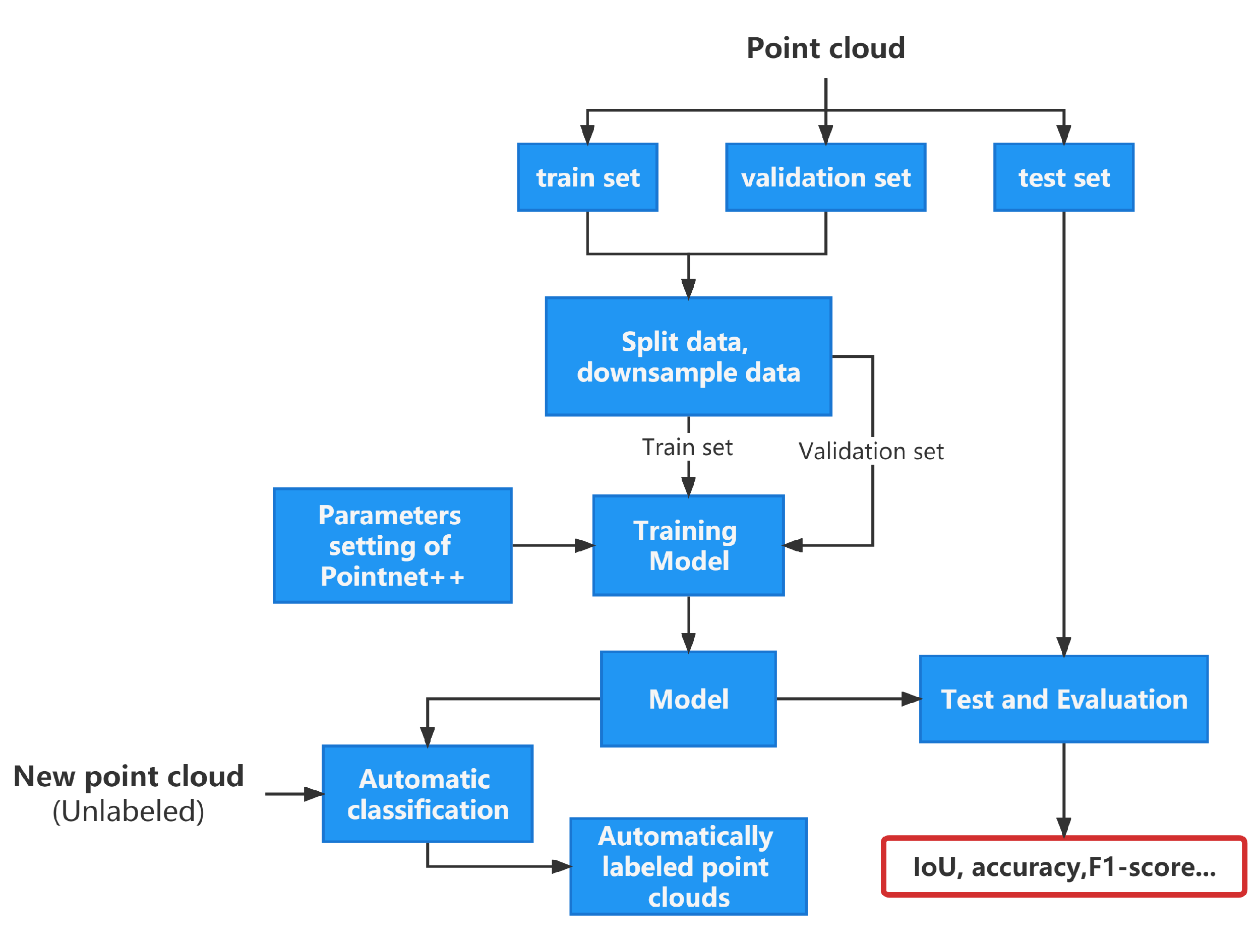
The classification based on deep learning, abbreviated as DPCC, can be divided into two types according to the input to the neural network. Whereas the first method converts the point cloud to another format as input (two-dimensional images or 3D voxels), the second one makes use of the original point cloud to avoid an increase in data volume and a loss of information during the conversion. In this contribution, we use an extension of PointNet [32], which is a deep learning point cloud classification/segmentation algorithm that utilizes the scattered point cloud directly as input. PointNet++ uses neighborhood information for feature extraction to face the generalization ability of this algorithm in complex scenarios. The idea behind PointNet++ is to first divide the point set into multiple overlapping subsets in space and use PointNet to extract fine local features from each subset. This process is repeated several times in a hierarchical manner, i.e., the output point set of each layer is used as the input point set of the next layer. This multilayer process generates point sets that contain rich contextual information. The workflow is summarized in Figure 3. The first step splits and downsamples the large-scale TLS point cloud. The second step sets the parameters of PointNet++, such as the training epoch. The training of the model chosen is performed in the third step. The fourth step tests the trained model using the test data set. Finally, the fifth step quantitatively evaluates the test results, using the metrics presented in Section 2.3.

2.3. Metrics

Different evaluation metrics have been proposed to evaluate the effectiveness of classification and segmentation algorithms quantitatively [42]. These evaluation metrics include accuracy, F1 score, and Intersection over Union (IoU). They are based on the values of true positive (TP), true negative (TN), false positive (FP), and false negative (FN) (see Table 2 for the corresponding definitions).
The accuracy (Acc), IoU, and F1 score can be computed from the values presented in Table 2. They evaluate the classification algorithm’s performance for each class. In order to measure the classification algorithm as a whole, three metrics will be used additionally. They are called mean IoU (mIoU), overall accuracy (OA), and mAcc. We refer to [42] for the corresponding formula and further mention that:
  • Accuracy indicates the number of samples that are correctly predicted divided by the number of all samples. The mAcc means the average of Acc values for each category.
  • IoU represents the intersection of predicted and true labels divided by the union of predicted and true labels [30]. In general, the larger the value of IoU, the better the classifier will be. The mIoU represents the average of the IoU values for each category.
  • The F1 score is the harmonic mean of the precision and recall. Precision represents the proportion of samples predicted to be positive cases that are actually positive cases. Recall is the proportion of correctly predicted positive cases to all true positive cases and is used as a measure of the classifier’s ability to identify positive cases.
  • OA represents the number of samples correctly classified as positive cases in all categories as a percentage of the total number of samples.

3. Results

We quantitatively test the various point cloud classification/segmentation algorithms described in Section 2 using a TLS point cloud from a landslide monitoring experiment that took place in Austria. After a short description of the experiment and an explanation of the pre-processing steps, we compare the various algorithms using the metrics defined in Section 2.3. Please note that all calculations were performed using the same hardware device with an AMD Ryzen 7 3700X CPU, 32G DDR4 running memory and a NVIDIA GeForce RTX2060 SUPER 8G graphics card.

3.1. Software

The point cloud labeling and division in the data preparation step were performed using CloudCompare [44]. CloudCompare is an easy-to-use, open source, 3D point cloud processing software with good visualization tools. We also used the software MATLAB 2021b [45] for the classification process, which includes the full process of algorithm operation and quantitative evaluation as well as the output of the point cloud processed. More specifically, we used the Deep Learning Toolbox (for setting up and training machine learning algorithms), the Computer Vision Toolbox (to visualize point clouds), and the LiDAR Toolbox Computer Vision Toolbox (for point cloud data reading, segmentation processing and other related tasks).

3.2. Description of the Data Set

3.2.1. Experiment

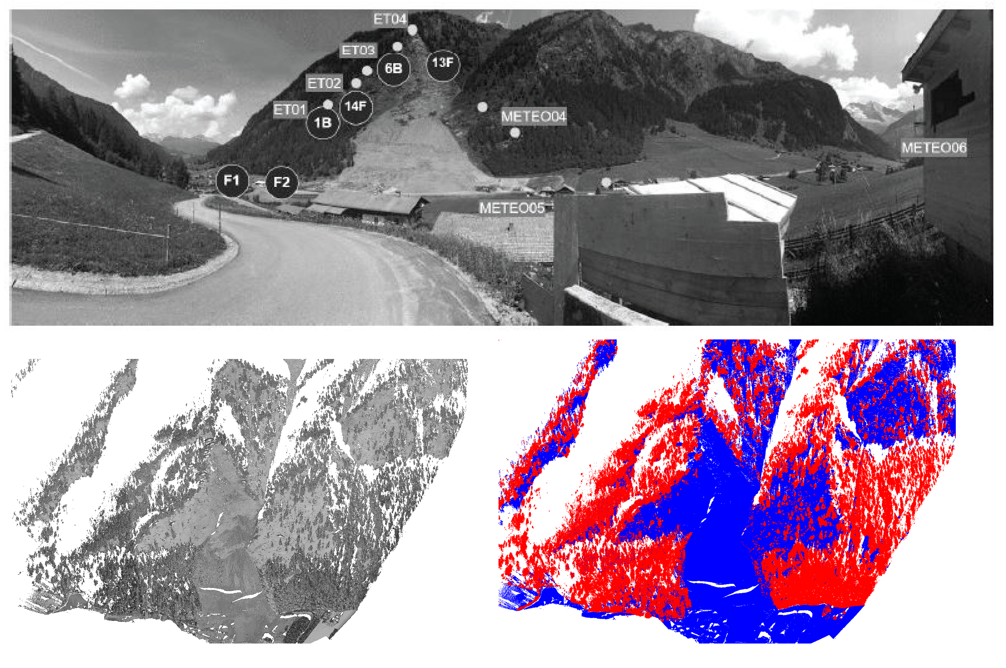
The data set used in this contribution was recorded in the Valsertal region in Austria as part of HORIZON 2020 via the Research Fund for Coal and Steel funded research project i2MON—“Integrated Impact MONitoring for the detection of ground and surface displacements caused by coal mining”, and is described in a dedicated publication [3] (also see [33]). The TLS under consideration is a long-range scanner, the RIEGL VZ-2000i [46]. The latter is able to measure objects with a very high accuracy (5 mm at 100 m) up to a range of 2500 m contact-free. Specific pre-processing is applied to improve the temporal discretization and enhances reliability to a high degree, making this TLS suitable for application in, for example, near-continuous monitoring of landslides. Here, this long-range TLS allows the analysis of deformation for safeguard applications. A picture of the scene recorded is shown in Figure 4, top. The original point cloud was recorded on 20 August 2020, and is presented in Figure 4, bottom left.

3.2.2. Pre-Processing

The point cloud under consideration contains about 15 million points in total. After manual classification using mainly the intensity value, we identified about 9 million containing vegetation (non-ground) points, as depicted in Figure 4, bottom right.
The supervised learning algorithm necessitates dividing the point cloud into a training set, a test set, and a validation set.
  • The training set is the data set used for model training [47].
  • The validation set is the data set used to evaluate the performance of the current model during training and tune the parameters.
  • The test set is the data set used to evaluate the model performance after the model training has been completed.
Unfortunately, there is no absolutely optimal division strategy. We have chosen 3% of the point cloud for the test set and 97% for the validation and test, based on the fact that the point cloud contains more than 10 million points, and following [47]. We further mention that a balance between the number of classes is mandatory when dividing the data to avoid one class with a much larger number than the others. In addition to the point cloud used for training and testing, a pre-processed point cloud needs to be divided to find a single-scale k n value. This point cloud is a small partition from the training point cloud. The data division is described in Table 3.

3.3. Classification

3.3.1. Parameters Selected

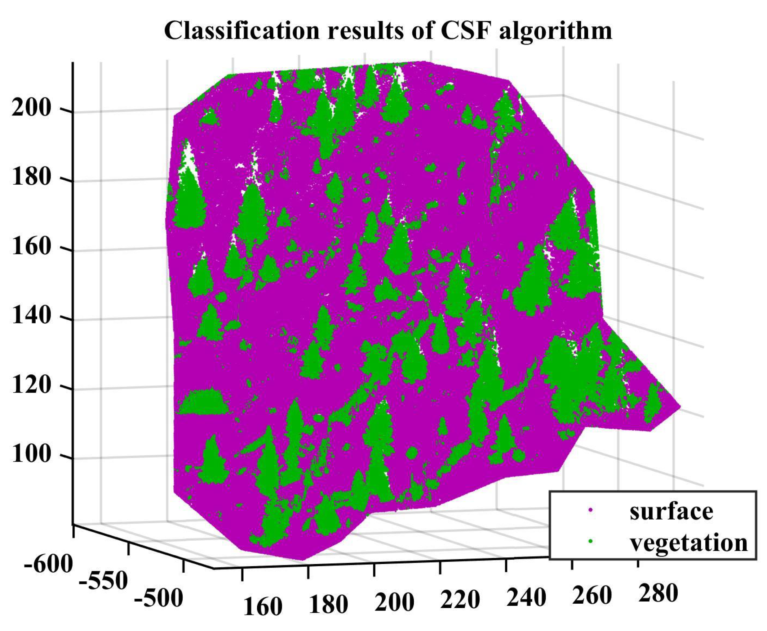
The use of the CSF and SMRF algorithms starts with the adaptation of the parameters to the point cloud. When the accuracy of the algorithm no longer significantly improves in the process of adjusting the parameters, the current parameters are output. They are presented in Table 4 and Table 5, respectively. An example of the classified point cloud is shown in Figure 5.
The values found for the single scale are 47, 53, 60, and 54 for the classifier DTC, RFC, DAC, and NNC, respectively (see Section 2.2.2).
The training parameters of PointNet++ are the training epoch, the validation frequency, and the learning rate, to cite but a few. They need to be tested several times before selecting the most suitable ones, as presented in Table 6.

3.3.2. Results

We have chosen to compare the various algorithms from two perspectives: their classification performance and their running time.

Classification Performance of Algorithms

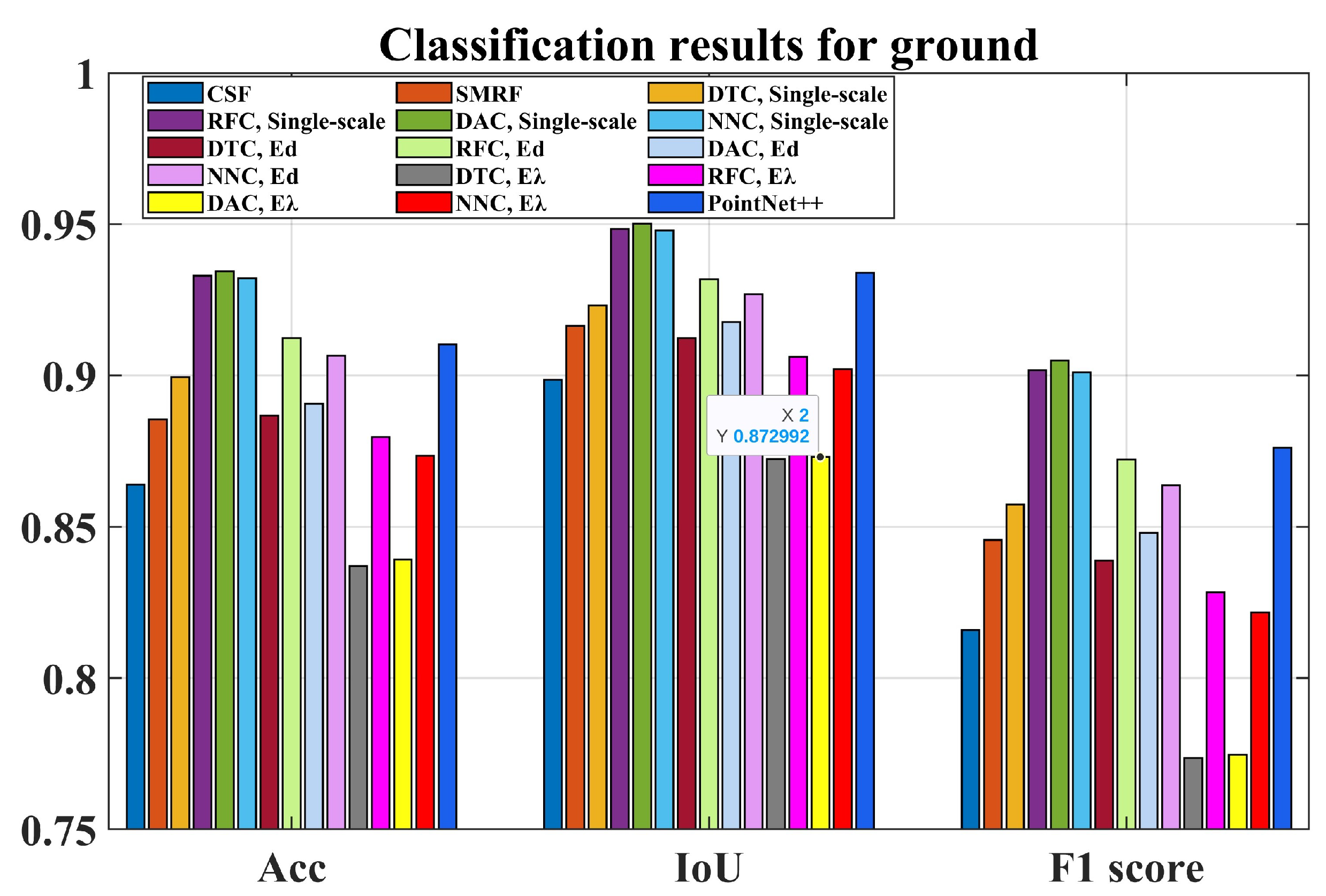
Figure 6 summarizes the classification results for the ground based on the Acc, IoU, and F1 score metrics (see Section 2.3). We note that among the FPCC algorithms, SMRF performs better than CSF for all metrics with a difference of approximately 0.02. Regarding the MLPCC methods, the performance of the single-scale algorithms is generally better than that of the methods based on multiple scale. Here, the Ed-based method seems slightly superior compared to the E λ -based method, with a difference of around 0.02–0.05 for the DAC/F1 score. The classification result from PointNet++ outperforms the FPCC algorithm and most of the MLPCC methods based on multiscales, but remains worthier than the DAC, RFC, and NNC algorithms based on a single scale. The difference reaches up to 0.1 compared, for example, to the DAC method with E λ for the F1 score.
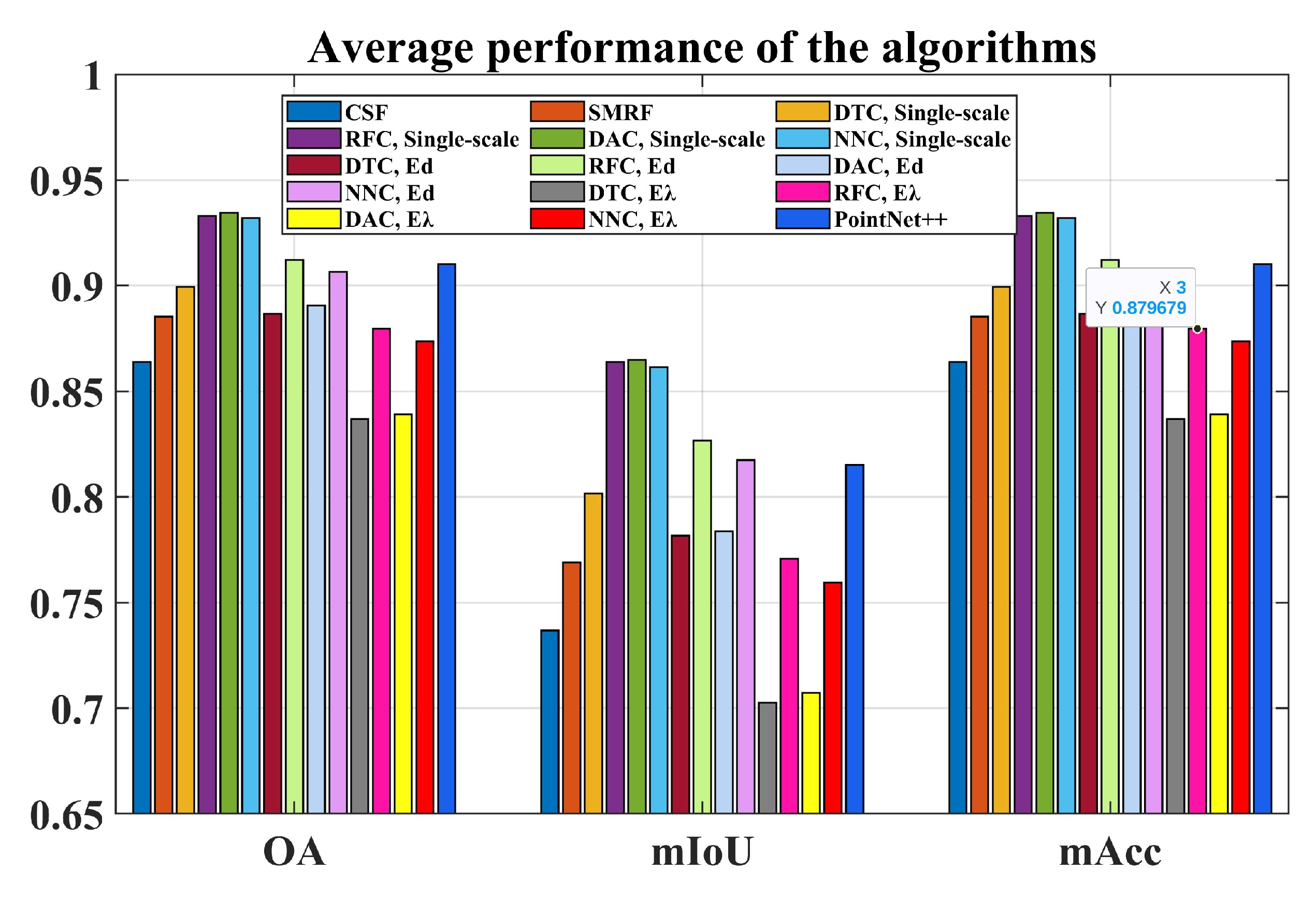
Figure 7 describes the average classification results of each algorithm based on the OA, mIoU, and mAcc for classifying ground points. Here, the SMRF algorithm performs slightly better than the CSF algorithm in all metrics (a difference of approximately 0.02). Regarding the MLPCC algorithm based on the single-scale k n , the average classification ability of NNC, RFC, and DAC is very similar compared to the DTC classification algorithm. However, when the k n value is computed with either the Ed or E λ method, the classification performance of the DAC algorithm decreases significantly compared to the RFC and NNC algorithms (0.05 for the OA and 0.1 for the F1 score). From this perspective, the RFC and NNC algorithms outperform the DAC algorithm. Regarding the DPCC algorithm, the average classification performance of PointNet++ is in the middle to upper range of these classification algorithms. It performs 0.02 worthier than the single-scale method RFC, DAC, and NNC algorithms for the OA and mAcc metric and 0.05 for the mIoU. To summarize the results of Figure 7, the classification performance of MLPCC based on single scale is better than that of DPCC, which is itself better than that of the FPCC algorithm for the average metrics.

Running Time of the Algorithms

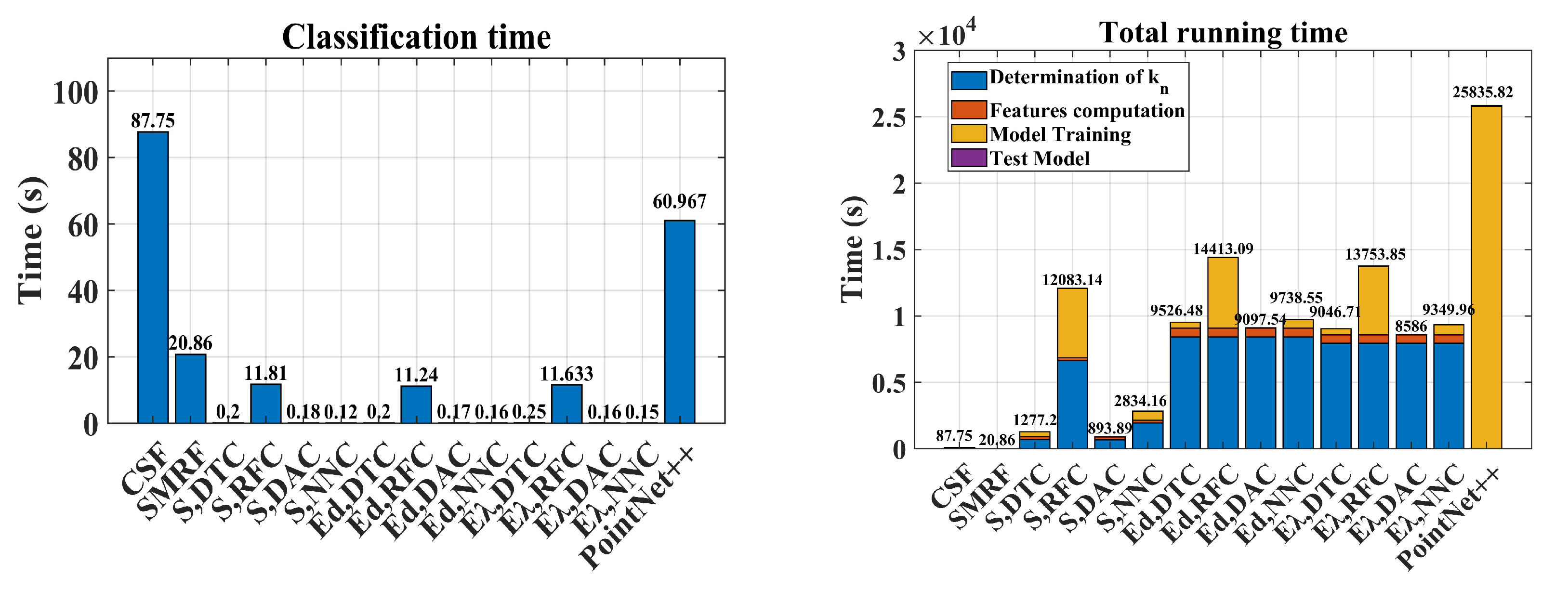
A summary of the running times of the algorithms is provided in Figure 8. Here, we define the running time of the FPCC algorithm as the time taken to perform the point cloud classification. Regarding the MLPCC algorithm, this time includes the time to determine k n , compute the point cloud features, train the model and use the model for point cloud classification. Regarding the DPCC algorithm, this time includes the training time of the model and the time to classify the point cloud using the model.
A detailed analysis of the running time is provided in Figure 8 (right). As expected, the FPCC algorithms have the shortest running time and the DPCC algorithm the longest one. Here, the determination of the k n value is shown to be time-consuming. Exemplarily, the RFC algorithm takes more than 50% of the total running time in determining the k n values and training the model compared with DTC and NNC methods, which are one-third faster than the RFC, independently of whether the E λ or the Ed method is used. Almost all of the computing time for the PointNet++ algorithm (which is more than two times higher than for the other algorithms) is used for model training. This method is, thus, less appealing than the other one regarding its computational performance.
The classification time is investigated more specifically in Figure 8 (left). As expected, the DTC, DAC, and NNC algorithms had the shortest classification times, i.e., 0.2 s in this case study. The RFC was slightly slower than these three algorithms and took about 11 s to classify. The SMRF algorithm needed twice as long, i.e., about 20 s. The slowest classification algorithms were PointNet++ and CSF, taking 60 and 87 s, respectively, to classify. Here, the bottleneck of the CSF is most probably the distance computation. However, regarding the total running time, the simplicity of the algorithm, and for both the data sets under consideration and the classification task, the filtering methods were the fastest overall.

3.3.3. Application: Surface Fitting

In this section, we show an application using the classified point cloud for surface approximation. The underlying application would be a deformation analysis from a near-continuous monitoring as in [11,48]. Here, distances can be easily computed based on the approximated surfaces, and mathematical spatiotemporal volumes can help visualizing changes by reducing data storage [49]. It is mandatory to extract only the ground for such applications in order not to approximate and compare the growth of the vegetation. As an example, we have chosen the CSF method to classify the point cloud based on its speed and accuracy, without a lack of generality regarding the other methods presented in the previous sections.
A subset of the point cloud containing approximately 1 million points has been chosen to perform the mathematical surface approximation with LR B-splines, see Figure 9 (left). We refer to [13] for more details on the procedure. The surface fitting algorithm chosen is called locally adaptive as it compares the difference in absolute value between the mathematical surface and the parametrized points inside a cell of a mesh using a given tolerance (the higher the tolerance, the coarser the approximation). If the tolerance is set too low, the risk of fitting the noise of the point cloud instead of its features exists. To face that challenge, the refinement is performed iteratively and stopped when, for example, the mean average distance starts to saturate. In our example, this value reaches 0.08 m for a tolerance of 0.5 m. We mention that the point clouds are noisy and the ground truth unknown, i.e., this value gives an indication of the adjusted point cloud to the mathematical surface and not about the details that can be detected. The maximum error was 4 m and the point cloud was reduced to 13,800 coefficients in less than 8 s. The result of the surface approximation after seven steps is depicted in Figure 9 (middle) with the corresponding LR mesh. The latter shows the cells where the adaptive refinement was performed (narrow gridding). Regarding the red points, the distance between the mathematical surface and the point cloud is maximum. This may be due to features that are difficult to approximate with a smooth mathematical surface, or the presence of non-ground points, such as any remaining unclassified vegetation. Thus, the number of points outside tolerance could come as a support to quantify the goodness of the classification algorithm. Further investigations are needed to validate such a promising approach.
Figure 9 (right) shows the final mathematical LR B-splines surface. We mention that the algorithm may try to extrapolate the gaps due to missing observations after the filtering of outliers and non-ground points, creating artificial oscillations. Accordingly, trimming is used, which is a popular method within the context of computed-aided design. This is illustrated by the voids, which correspond to the non-ground points eliminated prior to the surface approximation and non-fitted.

4. Discussion

We tested three different types of point cloud classification and segmentation methods in this contribution: FPCC, MLPCC, and DPCC. We selected popular and easy-to-use algorithms, which are available in either Python or MATLAB. Our classification task was to separate ground from non-ground points with the aim of performing a mathematical surface approximation of the point cloud for exemplary, rigorous statistical testing of the deformation between two point clouds. The data chosen were recorded in a mountainous region in Austria where landslides are known to occur. The advantages and drawbacks of each classification method are summarized in Table 7.
The following remarks can be drawn from Table 7:
  • Regarding the FPCC method, the advantage of the CSF and the SMRF algorithms compared to supervised classification algorithms comes from the fact that no a priori information (e.g., point cloud labels) is required to classify and segment the point clouds at hand. This property is very useful when the number of points is small and no prior information is available. Unfortunately, the parameters cannot be automatically adjusted in the simplest versions of the filtering algorithms.
  • Considering the MLPCC method, we tested the DAC, DTC, RFC, and NNC classification algorithms and three methods for the k n value determination. These algorithms have three disadvantages compared to FPCC methods: they require training data with a manual labeling, a manual extraction of features and the model needs to be trained. Consequently, the computational time is generally much higher than that of the FPCC method (except for DAC, where the training time is shorter). Fortunately, these methods have a good generalization ability, i.e., it is possible to classify point clouds using the trained model for the same type of classification task without parameter adjustment. The classification is fast and its accuracy is higher than with FPCC methods, provided that the k n value is chosen appropriately. The performance of the DAC algorithm based on the single scale in the OA metric example is about 5% higher than the SMRF algorithm and about 7% higher than the CSF algorithm. Compared to the DPCC method, the MLPCC method has three advantages: a higher classification accuracy when the best parameters are chosen, a shorter training time, i.e., the RFC with the longest training time is about 20,000 s less than the training time of PointNet++ for the point cloud under consideration, and its classification speed is fast. The RFC with the longest classification time takes about 50 s less than PointNet++. Compared to PointNet++, MLPCC requires manual extraction of point cloud features and, thus, large computational resources.
  • Regarding the DPCC method chosen (PointNet++), the 3D point cloud is used as input for the training of the model, and much is mandatory regarding the scattered and noisy TLS data. Compared to the MLPCC algorithm, no manual extraction of point cloud features is needed, the counterpart being the longer training time compared to the MLPCC algorithms. With respect to the FPCC methods, the DPCC has a higher classification accuracy and a better generalization ability, i.e., the parameters do not need to be adjusted after the model has been trained. Its disadvantage is the long training time.

5. Conclusions

In this contribution, we presented different methods for extracting non-ground points (here, vegetation) from TLS point clouds. We have chosen easy-to-understand and -implement strategies so that the reader can easily reproduce the results for similar applications. We have compared the algorithms chosen using a point cloud from a mountainous region in Austria with an underlying near-continuous monitoring application based on mathematical surfaces. We identified that the MLPCC algorithm based on the single scale has the best classifier regarding its computational time and classification performance. The CSF and SMRF were also interesting candidates due to their simplicity. The choice of the classification method is left to the user’s convenience depending on its needs and applications. The summary proposed in Table 7 can be used as orientation. We pointed out that the near-continuous recording with TLS makes a mathematical surface approximation of the point clouds a powerful alternative to working directly with the point clouds in standard software by reducing them to a few coefficients. Moreover, statistical testing of deformation can be performed based on the mathematical parameters. We have shown an example of how the filtered point cloud performs a mathematical surface modeling. The local refinement algorithm based on B-splines was chosen as particularly suitable for approximating smooth surfaces. Here, the voids due to the removal of non-ground points could be trimmed to avoid a drop in the approximated surface in domains with no points, thus, reducing the risk of oscillations in case of dense vegetation. Interpolation could be performed additionally. This topic is the subject of future research, as well as the possibility of using the results of the surface approximation itself to judge the goodness of the classification algorithms. Further applications using classified point clouds can include snow or sand dune monitoring. The extent to which those conclusions can be generalized to smoothed point clouds, as presented in, for example [50], needs further investigations.

Author Contributions

Conceptualization, G.K. and Z.Y.; methodology, G.K.; investigation and validation, G.K. and Z.Y.; writing—original draft preparation, G.K.; writing—review and editing, G.K., Z.Y. and D.C.-S. All authors have read and agreed to the published version of the manuscript.

Funding

Gaël Kermarrec is supported by the Deutsche Forschungsgemeinschaft under the project KE2453/2-1. Daniel Czerwonka-Schröder from DMT-group, Germany, provided the data set. This measurement campaign was supported by the Research Fund of the European Union for Coal and Steel [RFCS project number 800689 (2018)].

Data Availability Statement

The Austria data set used in this contribution can be made available on demand.

Acknowledgments

The publication of this article was funded by the Open Access Fund of the Leibniz Universität Hannover.

Conflicts of Interest

The authors declare no conflict of interest.

Abbreviations

3DThree-dimensional
AccAccuracy
CSFCloth simulation filtering
DACDiscriminant analysis classifier
DEMDigital elevation models
DPCCDeep learning point cloud classifier
DTCDecision tree classifier
FNFalse negative
FPFalse positive
FPCCFiltering point cloud classifier
IoUIntersection over union
LDALinear discriminant analysis
LidarLight detection and ranging
mAccMean accuracy
mIoUMean intersection over union
MLPMultilayer perception
MLPCCMachine learning point cloud classification
NNCNeural network classifier
OAOverall accuracy
OKBCOptimal K value finding method based on classification algorithms
RFCRandom forest classifier
SMRFSimple morphological filter
TLSTerrestrial laser scanning/scanner in context
TNTrue negative
TPTrue positive

References

  1. Vosselman, G.; Maas, H.G. Airborne and Terrestrial Laser Scanning; Whittles Publishing: Dunbeath, UK, 2010; pp. 1–318. [Google Scholar]
  2. Wu, C.; Yuan, Y.; Tang, Y.; Tian, B. Application of Terrestrial Laser Scanning (TLS) in the Architecture, Engineering and Construction (AEC) Industry. Sensors 2022, 22, 265. [Google Scholar] [CrossRef]
  3. Schröder, D.; Zimmermann, K.; Bock, S.; Klonowski, J. i2MON: Development of an integrated monitoring system for the detection of ground and surface displacements caused by coal mining. In Proceedings of the Conference: 2020 International Symposium on Slope Stability in Open Pit Mining and Civil Engineering, Cape Town, South Africa, 12–14 May 2020; pp. 353–366. [Google Scholar]
  4. Casagli, N.; Frodella, W.; Morelli, S.; Tofani, V.; Ciampalini, A.; Intrieri, E.; Raspini, F.; Rossi, G.; Tanteri, L.; Lu, P. Spaceborne, UAV and ground-based remote sensing techniques for landslide mapping, monitoring and early warning. Geoenviron. Disasters 2017, 4, 1–23. [Google Scholar] [CrossRef]
  5. Anders, K.; Winiwarter, L.; Höfle, B. Improving Change Analysis From Near-Continuous 3D Time Series by Considering Full Temporal Information. IEEE Geosci. Remote Sens. Lett. 2022, 19, 1–5. [Google Scholar] [CrossRef]
  6. Anders, K.; Winiwarter, L.; Mara, H.; Lindenbergh, R.; Vos, S.E.; Höfle, B. Fully automatic spatiotemporal segmentation of 3D LiDAR time series for the extraction of natural surface changes. ISPRS J. Photogramm. Remote Sens. 2021, 173, 297–308. [Google Scholar] [CrossRef]
  7. Rychkov, I.; Brasington, J.; Vericat, D. Computational and methodological aspects of terrestrial surface analysis based on point clouds. Comput. Geosci. 2012, 42, 64–70. [Google Scholar] [CrossRef]
  8. Wunderlich, T.; Niemeier, W.; Wujanz, D.; Holst, C.; Neitzel, F.; Kuhlmann, H. Areal Deformation Analysis from TLS Point Clouds—The Challenge. AVN Allg. Vermess. Nachrichten 2016, 123, 340–351. [Google Scholar]
  9. Mukupa, W.; Roberts, G.W.; Hancock, C.M.; Al-Manasir, K. A review of the use of terrestrial laser scanning application for change detection and deformation monitoring of structures. Surv. Rev. 2017, 49, 99–116. [Google Scholar] [CrossRef]
  10. Barbarella, M.; Fiani, M.; Lugli, A. Uncertainty in terrestrial laser scanner surveys of landslides. Remote Sens. 2017, 9, 113. [Google Scholar] [CrossRef] [Green Version]
  11. Kermarrec, G.; Kargoll, B.; Alkhatib, H. Deformation Analysis Using B-Spline Surface with Correlated Terrestrial Laser Scanner Observations—A Bridge Under Load. Remote Sens. 2020, 12, 829. [Google Scholar] [CrossRef] [Green Version]
  12. Kermarrec, G.; Morgenstern, P. Multilevel T-spline Approximation for Scattered Observations with Application to Land Remote Sensing. Comput.-Aided Des. 2022, 146, 103193. [Google Scholar] [CrossRef]
  13. Skytt, V.; Kermarrec, G.; Dokken, T. LR B-splines to approximate bathymetry datasets: An improved statistical criterion to judge the goodness of fit. Int. J. Appl. Earth Obs. Geoinf. 2022, 112, 102894. [Google Scholar] [CrossRef]
  14. Bracco, C.; Giannelli, C.; Großmann, D.; Imperatore, S.; Mokriš, D.; Sestini, A. THB-spline approximations for turbine blade design with local B-spline approximations. In Mathematical and Computational Methods for Modelling, Approximation and Simulation; Springer: Berlin/Heidelberg, Germany, 2022; pp. 63–82. [Google Scholar]
  15. Raschhofer, J.; Kerekes, G.; Harmening, C.; Neuner, H.; Schwieger, V. Estimating Control Points for B-Spline Surfaces Using Fully Populated Synthetic Variance–Covariance Matrices for TLS Point Clouds. Remote Sens. 2021, 13, 3124. [Google Scholar] [CrossRef]
  16. Harmening, C. Spatio-Temporal Deformation Analysis Using Enhanced B-Spline Models of Laser Scanning Point Clouds. Ph.D. Thesis, Department für Geodäsie und Geoinformation, Wien, Austria, 2020. [Google Scholar]
  17. Stumvoll, M.; Schmaltz, E.; Glade, T. Dynamic characterization of a slow-moving landslide system—Assessing the challenges of small process scales utilizing multi-temporal TLS data. Geomorphology 2021, 389, 107803. [Google Scholar] [CrossRef]
  18. Niemeyer, J.; Rottensteiner, F.; Soergel, U. Contextual classification of lidar data and building object detection in urban areas. ISPRS J. Photogramm. Remote Sens. 2014, 87, 152–165. [Google Scholar] [CrossRef]
  19. Brodu, N.; Lague, D. 3D terrestrial lidar data classification of complex natural scenes using a multi-scale dimensionality criterion: Applications in geomorphology. ISPRS J. Photogramm. Remote Sens. 2012, 68, 121–134. [Google Scholar] [CrossRef] [Green Version]
  20. Dorninger, P.; Székely, B.; Zámolyi, A.; Roncat, A. Automated detection and interpretation of geomorphic features in LiDAR point clouds. Vermess. Geoinf. 2011, 2, 60–69. [Google Scholar]
  21. Monserrat, O.; Crosetto, M. Deformation measurement using terrestrial laser scanning data and least squares 3D surface matching. ISPRS J. Photogramm. Remote Sens. 2008, 63, 142–154. [Google Scholar] [CrossRef]
  22. Mayr, A.; Rutzinger, M.; Bremer, M.; Oude Elberink, S.; Stumpf, F.; Geitner, C. Object-based classification of terrestrial laser scanning point clouds for landslide monitoring. Photogramm. Rec. 2017, 32, 377–397. [Google Scholar] [CrossRef] [Green Version]
  23. Li, Z.; Zhang, L.; Tong, X.; Du, B.; Yuebin, W.; Zhang, L.; Zhang, Z.; Liu, H.; Mei, J.; Xing, X.; et al. A Three-Step Approach for TLS Point Cloud Classification. IEEE Trans. Geosci. Remote Sens. 2016, 1–13. [Google Scholar] [CrossRef]
  24. Pingel, T.J.; Clarke, K.C.; McBride, W.A. An improved simple morphological filter for the terrain classification of airborne LIDAR data. Isprs J. Photogramm. Remote Sens. 2013, 77, 21–30. [Google Scholar] [CrossRef]
  25. Zhang, W.; Qi, J.; Wan, P.; Wang, H.; Xie, D.; Wang, X.; Yan, G. An Easy-to-Use Airborne LiDAR Data Filtering Method Based on Cloth Simulation. Remote Sens. 2016, 8, 501. [Google Scholar] [CrossRef]
  26. Wujanz, D.; Burger, M.; Tschirschwitz, F.; Nietzschmann, T.; Neitzel, F.; Kersten, T.P. Determination of Intensity-Based Stochastic Models for Terrestrial Laser Scanners Utilising 3D-Point Clouds. Sensors 2018, 18, 2187. [Google Scholar] [CrossRef] [PubMed]
  27. Schmitz, B.; Holst, C.; Medic, T.; Lichti, D.D.; Kuhlmann, H. How to Efficiently Determine the Range Precision of 3D Terrestrial Laser Scanners. Sensors 2019, 19, 1466. [Google Scholar] [CrossRef] [PubMed] [Green Version]
  28. Weinmann, M.; Jutzi, B.; Mallet, C. Semantic 3D scene interpretation: A framework combining optimal neighborhood size selection with relevant features. ISPRS Ann. Photogramm. Remote Sens. Spat. Inf. Sci. 2014, II-3, 181–188. [Google Scholar] [CrossRef] [Green Version]
  29. Biau, G.; Scornet, E. A Random Forest Guided Tour. arXiv 2015, arXiv:1511.05741. [Google Scholar] [CrossRef] [Green Version]
  30. Tanimoto, T. An Elementary Mathematical Theory of Classification and Prediction; International Business Machines Corporation: Hongkong, China, 1958. [Google Scholar]
  31. Wang, Y.; Shi, T.; Yun, P.; Tai, L.; Liu, M. PointSeg: Real-Time Semantic Segmentation Based on 3D LiDAR Point Cloud. arXiv 2018, arXiv:1807.06288. [Google Scholar]
  32. Pei, W.; Yinglei, C.; Wangsheng, Y. Point Cloud Classification Methods Based on Deep Learning: A Review. Laser Optoelectron. Progress 2021, 58, 160003. [Google Scholar]
  33. Schröder, D.; Anders, K.; Winiwarter, L.; Wujanz, D. Permanent terrestrial LiDAR monitoring in mining, natural hazard prevention and infrastructure protection—Chances, risks, and challenges: A case study of a rockfall in Tyrol, Austria. In Proceedings of the 5th Joint International Symposium on Deformation Monitoring (JISDM), Valencia, Spain, 20–22 June 2022. [Google Scholar] [CrossRef]
  34. Bentley, J.L. Multidimensional binary search trees used for associative searching. Commun. ACM 1975, 18, 509–517. [Google Scholar] [CrossRef]
  35. Michie, D.; Spiegelhalter, D.J.; Taylor, C.C.; Campbell, J. (Eds.) Machine Learning, Neural and Statistical Classification; Ellis Horwood: Chichester, UK, 1995. [Google Scholar]
  36. Kermarrec, G.; Alkhatib, H.; Neumann, I. On the Sensitivity of the Parameters of the Intensity-Based Stochastic Model for Terrestrial Laser Scanner. Case Study: B-Spline Approximation. Sensors 2018, 18, 2964. [Google Scholar] [CrossRef] [Green Version]
  37. Weinmann, M.; Jutzi, B.; Mallet, C.; Weinmann, M. Geometric features and their relevance for 3D point cloud classification. ISPRS Ann. Photogramm. Remote Sens. Spat. Inf. Sci. 2017, IV-1/W1, 157–164. [Google Scholar] [CrossRef] [Green Version]
  38. Chen, C.; Guo, J.; Wu, H.; Li, Y.; Shi, B. Performance Comparison of Filtering Algorithms for High-Density Airborne LiDAR Point Clouds over Complex LandScapes. Remote Sens. 2021, 13, 2663. [Google Scholar] [CrossRef]
  39. Sabirova, A.; Rassabin, M.; Fedorenko, R.; Afanasyev, I. Ground Profile Recovery from Aerial 3D LiDAR-Based Maps. In Proceedings of the 2019 24th Conference of Open Innovations Association (FRUCT), Moscow, Russia, 8–12 April 2019; pp. 367–374. [Google Scholar] [CrossRef] [Green Version]
  40. Zhang, K.; Chen, S.; Whitman, D.; Shyu, M.L.; Yan, J.; Zhang, C. A progressive morphological filter for removing nonground measurements from airborne LIDAR data. IEEE Trans. Geosci. Remote. Sens. 2003, 41, 872–882. [Google Scholar] [CrossRef]
  41. Demantke, J.; Mallet, C.; David, N.; Vallet, B. Dimensionality based scale selection in 3D Lidar point clouds. Int. Arch. Photogramm. Remote Sens. Spat. Inf. Sci. 2011, 38-5/W12, 97–102. [Google Scholar] [CrossRef] [Green Version]
  42. Aggarwal, C.C. Data Classification: Algorithms and Applications, 1st ed.; Chapman & Hall: London, UK, 2014. [Google Scholar]
  43. Fürnkranz, J. Decision Tree. In Encyclopedia of Machine Learning; Springer: Boston, MA, USA, 2010; pp. 263–267. [Google Scholar] [CrossRef]
  44. CloudCompare [GPL Software], Version 2.12; Free Software Foundation: Boston, MA, USA, 1989.
  45. MATLAB; The MathWorks, Inc.: Natick, MA, USA, 1970.
  46. RIEGL VZ-2000i. Available online: http://www.riegl.com/nc/products/terrestrial-scanning/produktdetail/product/scanner/58/ (accessed on 12 September 2022).
  47. Gareth, J.; Daniela, W.; Trevor, H.; Robert, T. An Introduction to Statistical Learning: With Applications in R; Spinger: Berlin/Heidelberg, Germany, 2013. [Google Scholar]
  48. Kermarrec, G.; Schild, N.; Hartmann, J. Fitting terrestrial laser scanner point clouds with T-splines: Local refinement strategy for rigid body motion. Remote Sens. 2021, 13, 2494. [Google Scholar] [CrossRef]
  49. Kermarrec, G.; Skytt, V.; Dokken, T. Surface Approximation of Coastal Regions: LR B-Spline for Detection of Deformation Pattern. ISPRS Ann. Photogramm. Remote Sens. Spat. Inf. Sci. 2022, 52, 119–126. [Google Scholar] [CrossRef]
  50. Anders, K.; Eberlein, S.; Höfle, B. Hourly Terrestrial Laser Scanning Point Clouds of Snow Cover in the Area of the Schneeferner, Zugspitze, Germany. 2022. Available online: https://doi.pangaea.de/10.1594/PANGAEA.941550 (accessed on 12 September 2022).
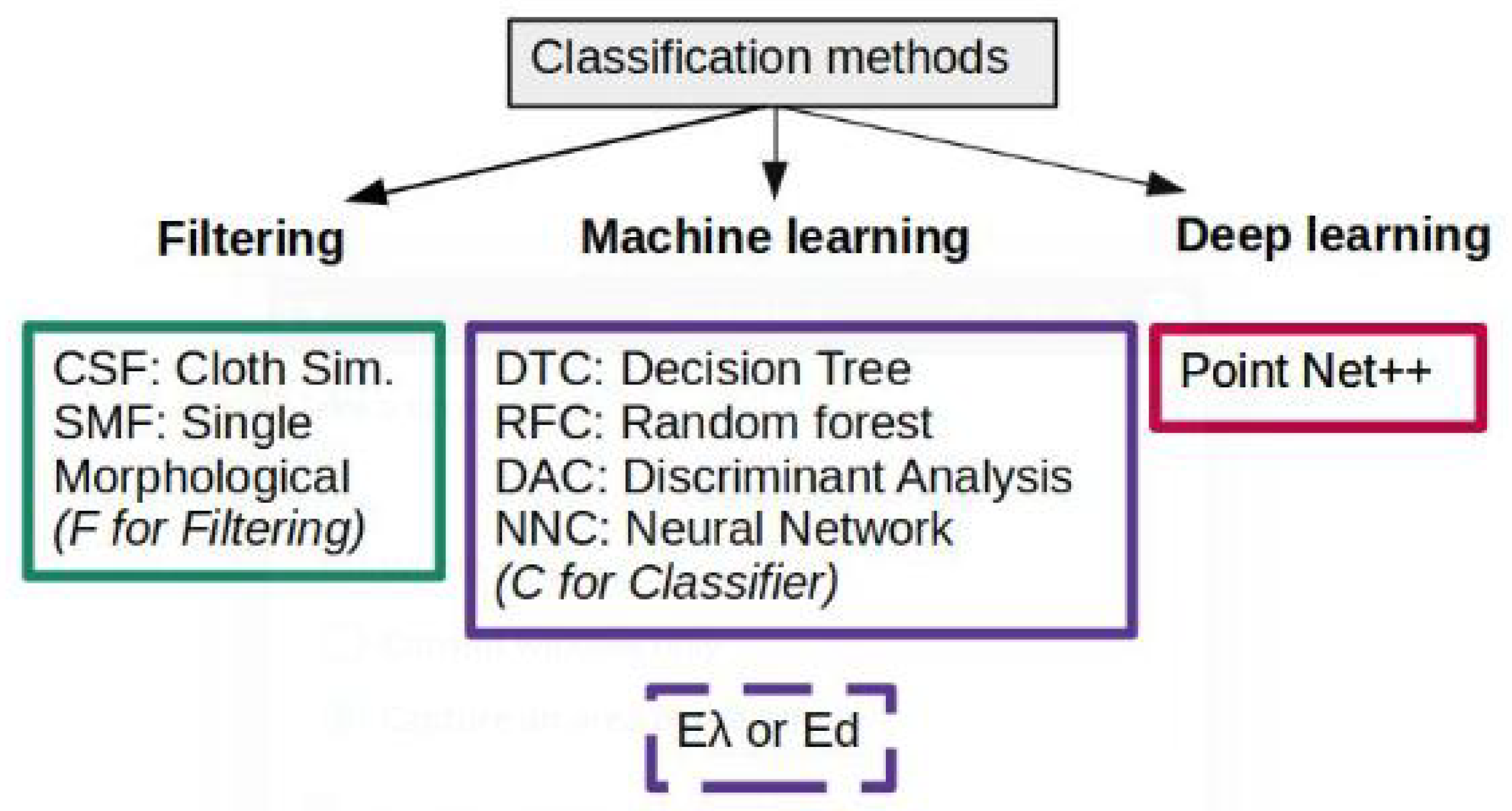
Figure 1. Summary of the methods tested in this contribution.
Remotesensing 14 05099 g001
Figure 2. Typical workflow of classification methods.
Remotesensing 14 05099 g002
Figure 3. Principle of PointNet++ for large-scale TLS point clouds.
Remotesensing 14 05099 g003
Figure 4. Top: View of the region under consideration. Bottom left: Visualization of the point cloud with the software CloudCompare. Bottom right: Results of the manual labeling (red: non-ground, blue: ground).
Remotesensing 14 05099 g004
Figure 5. Classification of the point cloud with CSF.
Remotesensing 14 05099 g005
Figure 6. Classification results: Acc, IoU, F1 score.
Remotesensing 14 05099 g006
Figure 7. Classification results: OA, mIoU, mAcc.
Remotesensing 14 05099 g007
Figure 8. Left: Running time for the classification only. Right: Total running time.
Remotesensing 14 05099 g008
Figure 9. Left: Domain selected for surface approximation. Middle: points colored according to the distance to the approximated surface, together with the LR mesh. Right: The trimmed surface after seven iterations.
Remotesensing 14 05099 g009
Table 1. Geometric features of a point p 0 with coordinates (x, y, z). k n is the number of nearest neighboring points. λ are the eigenvalues of the covariance matrix built from the k n points per descending order. Z refers to the z-coordinate, dr is the distance between the reference point and the best fitting plane computed on its nearest neighbors. rmax denotes the distance of the farthest point from the reference point among the k n neighboring points.
Feature nbFeature NameFormula
1Linearity λ 1 λ 2 λ 1
2Planarity λ 2 λ 3 λ 1
3Scattering λ 3 λ 1
4Omnivariance λ 1 λ 2 λ 3
5Anisotropy λ 1 λ 3 λ 1
6Eigenentropy i = 1 3 λ i ln λ i
7Sum of eigenvalues λ 1 + λ 2 + λ 3
8Change of curvature λ 3 λ 1 + λ 2 + λ 3
9Mean Z i = 1 k n + 1 Z i k n + 1
10Z variance i = 1 k n + 1 Z i m e a n ( Z ) k n + 1
11Maximum Z difference Z m a x Z m i n
12PCA1 λ 1 λ 1 + λ 2 + λ 3  
13PCA2 λ 2 λ 1 + λ 2 + λ 3
14Roughnessdr
15normal vector xnx
16normal vector yny
17normal vector znz
18Density k n + 1 4 / 3 r max
19Verticality1 − nz
Table 2. Definition of true positive (TP), true negative (TN), false positive (FP) and false negative (FN).
Definition 1.
TP:A test result correctly indicating the presence of a condition or characteristic.
FN:A test result wrongly indicating that a particular condition or attribute is absent.
FP:A test result wrongly indicating that a particular condition or attribute is present.
TN:A test result correctly indicating the absence of a condition or characteristic.
Table 3. Data division.
Vegetation PartSurface PartTotalProportion
Train set8,734,6145,685,38714,420,00193.47%
Test set188,582342,772531,3543.44%
Validation set171,756305,034476,7903.09%
Pre-train set41,80660,178101,98482.69%
Pre-test set533816,00721,34517.30%
Table 4. Parameter setting for CSF.
RigidnessTime StepGrid ResolutionDistance ThresholdHeight DifferenceMaximum Number of IterationsSteep Slope Fit Factor
Parameter Value10.7150.11.50.3500True
Table 5. Parameter setting for SMRF.
Surface GridSlope Value (%)Windows SizeSingle Elevation Difference Value
Parameter Value0.10.15900.001
Table 6. Parameter settings for PointNet++.
ParametersSettingsMeaning of Parameters
Number points10,000Fixed number of points per grid
Grid size (m) [20, 20]Size of the grid
Grid orientationYZDirection of the split
Max epochs20Epoch number
Validation frequency50Frequency of network validation
Initial learn rate0.0005Initial learning rate
L2 regularization0.01Factor for L2 regularization (weight decay)
Mini batch size6Size of the mini-batch to use for each training iteration
Learn rate drop factor0.1Factor for dropping the learning rate
Learn rate drop period10Number of epochs for dropping the learning rate
Gradient decay factor0.9Decay rate of gradient moving average
Squared gradient decay factor0.999Decay rate of squared gradient moving average
Number nearest neighbors20The number of nearest points in the downsampled point cloud for each point in the dense point cloud
Training time (s)25,774.86Time to train the model.
Test time (s)60.967Time to test the model
Table 7. Advantages and disadvantages of different algorithms.
FPCCMLPCCDPCC
Advantages
  • No prior information required.
  • Time to run the complete algorithm short.
  • Good generalization ability.
  • Fast classification speed.
  • High classification accuracy.
  • Good generalization ability.
  • Automatic extraction of point cloud features.
  • Relatively high classification accuracy.
Disadvantages
  • Each use requires parameter adjustment.
  • Relatively low classification accuracy.
  • Requires manual extraction of point cloud features
  • Large amount of computing resources for large point clouds.
  • Long training time.
  • Training data with labeling.
  • Long training time.
  • Classification speed is slow.
  • Requires training data with labeling.
Publisher’s Note: MDPI stays neutral with regard to jurisdictional claims in published maps and institutional affiliations.