Abstract
With the availability of low-cost, mass-market dual-frequency GNSS (Global Navigation Satellite System) receivers, standalone processing methods such as Precise Point Positioning (PPP) are no longer restricted to geodetic-grade GNSS equipment only. However, with cheaper equipment, data quality is expected to degrade. This same principle also affects low-cost GNSS antennas, which usually suffer from poorer multipath mitigation and higher antenna noise compared to their geodetic-grade counterparts. This work assesses the quality of a particular piece of low-cost GNSS equipment for real-time PPP and high-rate dynamic monitoring applications, such as strong-motion seismology. We assembled the u-blox ZED-F9P chip in a small and light-weight data logger. With observational data from static experiments—which are processed under kinematic conditions—we assess the precision and stability of the displacement estimates. We tested the impact of different multi-band antenna types, including geodetic medium-grade helical-type (JAVAD GrAnt-G3T), as well as a low-cost helical (Ardusimple AS-ANT2B-CAL) and a patch-type (u-blox ANN-MB) antenna. Besides static tests for the assessment of displacement precision, strong-motion dynamic ground movements are simulated with a robot arm. For cross-validation, we collected measurements with a JAVAD SIGMA G3T geodetic-grade receiver. In terms of precision, we cross-compare the results of three different dual-frequency, real-time PPP solutions: (1) an ambiguity-float solution using the Centre National d’Études Spatiales (CNES) open-source software, (2) an ambiguity-float and an AR (ambiguity-resolved) solution using the raPPPid software from TU Vienna, and (3) and a PPP-RTK solution using the u-blox PointPerfect positioning service. We show that, even with low-cost GNSS equipment, it is possible to obtain a precision of one centimeter. We conclude that these devices provide an excellent basis for the densification of existing GNSS monitoring networks, as needed for strong-motion seismology and earthquake-early-warning.
1. Introduction
Today, users have access to the signals of four major Global Navigation Satellite Systems (GNSS) [1,2]. Typically, more than 20 satellites are visible at any time for a receiver under an open sky. This allows reaching positioning precision down to centimeters in real-time (e.g., Alkan et al. [3]). To achieve such precision with standalone receivers, to date, it has been necessary to use expensive high-grade GNSS equipment that allows the processing of GNSS signals in two or more frequency bands in a real-time precise point positioning (PPP) mode. Since the IGS (International GNSS Service) first launched a pilot project on a real-time PPP corrections service in 2007, numerous studies have analyzed the quality of the PPP in terms of accuracy and convergence times (e.g., Chen et al. [4], Hadas [5], Wang et al. [6], Elsobeiey and Al-Harbi [7]). Dual-frequency GNSS observations enable PPP, since the effects of the ionosphere can be considered, for example by forming the ionosphere-free linear combination (IF LC) [8,9]. A bottleneck of PPP positioning are long convergence times with usually tens of minutes to reach cm-level accuracy (Yu and Gao [10], Leandro et al. [11]). To overcome this, PPP-RTK (Real-Time Kinematic) was developed [12]—besides the correction data for satellite orbits and clocks, this method uses satellite phase (and code) bias corrections that allow for integer ambiguity resolution (AR) (e.g., Teunissen and Khodabandeh [13]), or even real-time atmospheric correction data (e.g., Li et al. [14]), enabling AR within a few epochs. In addtion to PPP-RTK, a term commonly used in the community is real-time PPP-AR, especially when only code and phase bias correction data are used. Recently, more and more institutions have started to provide satellite products suitable for PPP-AR; Glaner and Weber [15] provide an overview, for example. The approaches introduced by Laurichesse et al. [16] and Ge et al. [17] are mainly applied, enabling the PPP user to fix the ambiguities of the IF LC in two steps (Wide-Lane (WL) and Narrow-Lane (NL) fixing). Ge et al. [17] developed a method to determine uncalibrated phase delays (UPDs) for the WL and NL ambiguity in a network solution. These WL and NL UPDs are forwarded to the user and allow fixing the single-differenced ambiguities between satellites during the PPP solution. Laurichesse et al. [16] used the same decomposition in WL and NL as Ge et al. [17], but the undifferenced ambiguities are fixed directly to an integer in the network solution. Unlike Ge et al. [17], this strategy assimilates the NL UPDs into the clock estimates. Consequently, this strategy is called the integer recovery clock method, and the PPP user has only to apply WL UPDs. Despite these different strategies, producing a combined PPP-AR satellite product is possible [13] and was tested for GPS [18].
Low-cost single-frequency GNSS has proven to provide sufficient precision for many applications in geodetic, navigational and geophysical monitoring, with its strengths in relative positioning methods such as Real Time Kinematic (RTK) (e.g., Tsakiri et al. [19], Lu et al. [20], Kenner et al. [21], Cina and Piras [22], Tsakiri et al. [23], Garrido-Carretero et al. [24], Odolinski and Teunissen [25]). A few years ago, low-cost dual-frequency receivers became available—the Swiss chip manufacturer u-blox launched the dual-frequency GNSS chipset ZED-F9P, which typically comes at a price of less than 200 USD. Hamza et al. [26] tested a u-blox ZED-F9P with different uncalibrated low-cost helix antennas of type “Tallysman TW3882” and of type “Survey” (which relates to the AS-ANT2B-CAL, called ASANT in the following) against calibrated geodetic-grade antennas. For zero-baseline and short-baseline tests using the open-source RTKLIB GNSS software package [27], they could show that precision and accuracy can reach mm-level with low-cost equipment as well. They concluded that, although geodetic equipment still shows better performance, not only are the costs much lower, but also the performance is reasonable for many geodetic applications. Using the same processing modes, Hamza et al. [28] also showed that with these low-cost antennas sub-centimeter displacements can be detected for the short-baseline case, and down to few centimeters using PPP in post-processing. Regarding accuracy, they also outlined the positive effect on accuracy when accounting for available antenna calibration for the ASANT antenna. For crustal deformation studies, Tunini et al. [29] compared the performance of u-blox ZED-F9P to geodetic receivers, when being attached to the same geodetic-grade antennas. They concluded that the results for both receiver types are largely comparable, with no significant trade-offs in quality for the low-cost receiver. For RTK on short and medium-length baselines, Janos et al. [30] recently demonstrated that the ZED-F9P can be successfully used for applications requiring positioning accuracy of few centimeters. Wielgocka et al. [31] demonstrated that PPP solutions with u-blox low-cost equipment (ZED-F9P and ANN-MB patch antenna) can reach an accuracy of few centimeters for PPP in post-processing mode, after a certain convergence time. With the same equipment, but using a single-frequency PPP approach Paziewski [32] concluded that still multipath is the limiting error source for GNSS equipment. The value of u-blox dual-frequency equipment was also demonstrated for tropospheric delay estimation, where Krietemeyer et al. [33] showed that by including calibrations for low-cost antennas, the error regarding geodetic solutions can be at the sub-centimeter level. For the GNSS processing they used RTKLIB in a static mode. Nie et al. [34] also used u-blox dual-frequency equipment to demonstrate decimeter-level accuracy for kinematic trajectory estimation using real-time PPP. The authors could decrease the convergence time by using precise ionospheric products.
Over the past few decades, GNSS geomonitoring has become an important tool for earth sciences and engineering: beyond traditional applications in measuring long-term ground motions such as plate tectonics or postglacial uplift, real-time and high-rate kinematic GNSS displacements now significantly contribute to the monitoring of earthquakes, landslides or civil structures (e.g., Bock and Wdowinski [35], Shen et al. [36]). For safety-critical applications—like earthquake early warning (EEW) or structural health monitoring—reliable and high-precision real-time GNSS displacements are becoming a central element. Unlike than seismometers, GNSS does not suffer from saturation effects and it directly measures displacements (instead of accelerations) [37]. For EEW, this makes it particularly important for magnitude estimation and rapid earthquake source characterization in great earthquakes [38,39], yet it can still be effective in moderate events since real-time GNSS displacements can resolve seismic waveforms down to the level of a centimeter component-wise. For such applications, as well as for monitoring stations in remote areas, relative positioning is not the option of first choice—an important issue for earthquake monitoring is that a nearby reference station will also be affected by the earthquake [40]. The Institute of Geodesy and Photogrammetry (IGP) of ETH Zurich runs GNSS geomonitoring stations in the Swiss alps, using single-frequency u-blox chips [41]. These solar-powered and autonomous stations have been upgraded with u-blox dual-frequency chips, which enables the application of real-time PPP and is particularly useful for EEW, or for real-time monitoring of the state of the troposphere. It was demonstrated that real-time PPP, and the so-derived seismic source parameters can come close to the quality obtained from postprocessed solutions (e.g., Dahmen et al. [39], Melgar et al. [42]). For GNSS real-time seismology, the short-term displacement precision is more important than the long-term accuracy or repeatability, since strong-motion displacements typically last for minutes only, even for strong earthquakes. In EEW, it is essential to have stations located near the source, because these are subject to strong motions [43]. A Swiss scientific consortium [44] gave the recommendation to densify GNSS networks with station distances of 10 to 20 km—the current station density of the Swiss high-grade GNSS network is about 40 to 60 km. A limiting factor for GNSS network densification with dual-frequency equipment is the price—a high-grade geodetic receiver and a high-grade antenna typically cost 20,000 to 30,000 USD per station. Consequently, these costs can be significantly reduced if low-cost equipment can be used.
In this work, we analyze the precision of high-rate and real-time kinematic PPP, when observations are collected with low-cost u-blox ZED-F9P receivers and different antennas. In view of real-time geohazard detection (such as EEW) and GNSS network densification, we see a need for studies analyzing the attainable displacement precision with these instruments. To our best knowledge, there is no such study that assesses the performance of the u-blox ZED-F9P for kinematic geomonitoring applications, whilst cross-comparing low-cost and a geodetic-grade antennas and using different GNSS processing software packages. This includes the low-cost ASANT antenna, as well as the u-blox PointPerfect real-time positioning service. Our precision assessment relies on static and dynamic experimental tests—the observations collected for the static tests are processed under kinematic conditions; therefore, we will refer to it as static kinematic in the following. Furthermore, we also cross-validate the results with data from the geodetic-grade JAVAD receiver. Our study is based on experiments of three different measurement sessions, spanning from spring 2021 to spring 2022. The central element of this work is an analysis of error characteristics of the real-time PPP displacement estimates—in terms of error magnitudes and stability of the data, the obtainable precision and the resolvability of strong ground motion. For the GNSS processing we use the software package “PPP-Wizard” from Centre National d’Études Spatiales (CNES) [45], the raPPPid software from TU Vienna [15], and the commercial-of-the-shelf PPP-RTK positioning software PointPerfect of the company u-blox [46].
This document is organized as follows: The Section on “Instrumentation and GNSS Processing” explains the measurement setups for the individual sessions, and important details on the GNSS processing are given. Based on the computed kinematic time series data, Section “Results and Discussion” then shows and discusses the most important findings of the static kinematic and dynamic experiments, with root mean square (RMS) amplitudes as the main quality indicator. We also touch noise characteristics of real-time PPP with low-cost instruments. Furthermore, in the main body of this text we refer to additional helpful results given in a supplementary material section. Based on the results and discussions, important conclusions are drawn, and a short outlook on further work is given.
2. Instrumentation and GNSS Processing
2.1. Instrumentation
Table 1 and Table 2 list some general specifications of the GNSS receivers and the antennas used for the experiments. It also shows the approximate price of the instruments (prices are considered without warranty, as found in Switzerland). The u-blox logger collects data in the L1, L2 and E5 band. The JAVAD SIGMA G3T receiver can collect observations additionally in the L5 frequency band. With both devices, all four major GNSS can be observed. The ZED-F9P (termed F9P in the following) samples with a maximum rate of 20 Hz. The JAVAD receiver samples with rates up to 100 Hz. The u-blox logger wears the ZED-F9P chip, and was assembled in our labs with material costs of around 350 USD (working time not included, the chip is about 150 to 200 USD). The price of the JAVAD SIGMA receiver is about 10,000 USD. Table 2 lists the specifications for the antennas. Basically, the u-blox multi-band antenna ANN-MB-00 measures at two frequencies (and E5). For sessions 2 and 3, we also tested the helical-type low-cost antenna Ardusimple “survey” AS-ANT2B-CAL (termed ASANT in the following). The geodetic medium-grade antenna JAVAD GrAnt-G3T can measure at three frequencies. The price is around 60 USD for the u-blox antenna, around 90 USD for the ASANT antenna and approx. 1500 USD for the JAVAD GrAnt3 antenna.

Table 1.
Specifications of the GNSS receivers used for the experiments (the price for the ZED-F9P relates to the material costs of the data logger).
Table 2.
Specifications of the GNSS antennas used for the experiments.
The internal multipath mitigation algorithm of the JAVAD receiver was turned on when collecting measurements. The u-blox ZED-F9P also uses techniques in the receiver’s signal correlators, that result in a reduction of multipath signals, comparable to those in geodetic-grade receivers (personal communication with u-blox support). Therefore, to a certain extent, multipath errors are expected to be mitigated in the receiver internal signal processing on both devices, but will still be present in the results. For the u-blox receiver, the u-center 21.05 was used to configure the u-blox’s RAWX binary data as output stream, which enables the collection of raw GNSS measurements. For both, the JAVAD and the u-blox receivers, the measurements were stored as binary files (in the proprietary formats) on the internal memory, and then converted to Rinex files afterwards using RTKLIB’s RTKCONV [27].
2.2. Measurement Sessions
2.2.1. Session 1: u-blox and JAVAD Equipment, Static Kinematic and Dynamic Tests
Figure 1 shows the setup that has been used for the static kinematic experiments for this first session. The measurements were taken in April 2021 on the roof of the HPV building of ETH Zurich, in an almost open-sky environment. However, also strong multipath has to be expected, caused by many adjacent buildings and walls. The station MON1 (Figure 1, left-hand side LHS) was equipped with the JAVAD GrAnt-G3T antenna (geodetic medium-grade), connected to the u-blox logger and the JAVAD receiver via a signal splitter (grey box). Station RAIL (Figure 1, right-hand side RHS) was equipped with the u-blox ANN-MB patch antenna, connected to u-blox data logger (another grey box). Station RAIL and MON1 were separated approximately 7 m apart from each other.
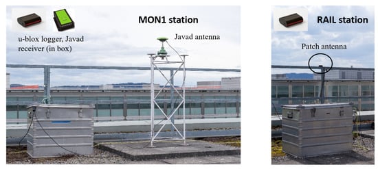
Figure 1.
Session 1: experimental setup for station “MON1” for the static kinematic tests (left-hand side) and station “RAIL” (right-hand side), located at the roof of ETH HPV building.
For the static kinematic tests, data were collected for the stations MON1 and RAIL from 14 to 16 April 2021, with a sampling rate of 1 Hz. The dynamic measurements were carried out on 27 April 2021, with the same GNSS hardware configuration that was used for the static experiments at station MON1 (JAVAD and u-blox receiver, splitter, JAVAD antenna), but with the antenna mounted on a mobile robot platform (Figure 2). In order to better resolve the seismic waveforms, a 5 Hz GNSS sampling rate was chosen for the dynamic tests. A KUKA Agilus KR 6 R900 sixx robot was used to simulate a seismic strong-motion waveform, for which a ground truth was available as well, measured in a well-defined robot coordinate system. We also used this robot for 6-degree-of-freedom seismology experiments fusing GNSS, accelerometer and rotational sensor data in a Kalman-filter approach [47].

Figure 2.
Experimental setup for the dynamic tests (session 1): a seismic strong-motion waveform was simulated using a KUKA robot arm. The same GNSS hardware was used as for the static kinematic test for station MON1.
Figure 3 shows the receiver and antenna combinations used for the experiments in session 1. For the dynamic tests, the same measurement setup was chosen as for the static kinematic test on MON1. GNSS measurements (code and phase) of GPS, GLONASS and Galileo were recorded and processed for the static experiment, and for the dynamic experiment, measurements of GPS and GLONASS were recorded and processed. The reason is that we encountered problems with data gaps for the u-blox receiver with 5 Hz sampling, when observing all constellations.

Figure 3.
Session 1: receiver and antenna combinations for the experimental tests. For the dynamic tests with the seismic strong-motion signal, only the configuration of MON1 was considered.
2.2.2. Session 2: u-blox and JAVAD Equipment, Helical Low-Cost Antenna, Static Kinematic Tests
Figure 4 shows the instrumental setup for the second session, measured in September 2021, again on the HPV building. The scene is now around station RAIL of session 1 (Figure 1, RHS; now LHS of Figure 4), for which again a u-blox logger and u-blox patch antenna were used. Station MON2 (Figure 4, middle) was equipped with the helical-type low-cost ASANT antenna. For the tripod station STA1 we used the JAVAD antenna. In the silver box of left of station MON2, both, the geodetic-grade JAVAD receiver, as well as the u-blox logger were placed, connected to the antenna via a signal splitter. The station RAIL was equipped with the u-blox logger.

Figure 4.
Session 2: experimental setup for station “RAIL”, “MON2” and “STA1” for the static kinematic tests, located at the roof of ETH HPV building.
Data were collected for all three stations from 10 to 13 September 2021, with a sampling rate of 1 Hz. Figure 5 shows the receiver and antenna combinations used for these experiments. GPS, GLONASS, and Galileo were recorded in this static kinematic tests.

Figure 5.
Session 2: receiver and antenna combinations for the experimental tests.
2.2.3. Session 3: u-blox Equipment, Helical Low-Cost Antenna, Static Kinematic Tests
Figure 6 shows the instrumental setup for the third session, measured in April and May 2022, on the HPV building, with a very similar setup as for session 2, but without the STA1 station. The purpose of this experiment was to test the performance of the u-blox commercial-of-the-shelf “PointPerfect” PPP-RTK positioning service, launched in autumn 2021. This service also allows for integer ambiguity resolution, and uses global and regional GNSS corrections [48]. For the tests, u-blox F9P loggers were placed in the nearby office, connected to two laptops. This was necessary to setup the internet connection for retrieving the PPP-RTK correction data, as well as for obtaining the precise positions using u-center 22.02, together with the F9P with a dedicated firmware. Data were collected for two stations over four sub-sessions (ranging from 27 April to the 4 May), with a sampling rate of 1 Hz. Figure 7 shows the receiver and antenna combinations used for these experiments. Likewise as for the other sessions GPS, GLONASS, and Galileo were measured for these tests.

Figure 6.
Session 3: experimental setup for station “RAIL” and “MON2” for the static kinematic tests for the u-blox PointPerfect tests, located at the roof of ETH HPV building.

Figure 7.
Session 3: receiver and antenna combinations for the experimental tests.
2.3. GNSS Processing
This section lists the different software packages and their setup, as used for the GNSS processing of the recorded data. To be as consistent as possible throughout the software packages and different receivers, we processed the same signals and same GNSS for all solutions (code and phase observations of L1 and L2 band, as well as E5 for Galileo, respectively) under the same configurations, whenever possible. We want to stress that it is not the goal of this study to compare the performance of different packages. Our aim is to present an analysis of the precision performance of kinematic real-time PPP with low-cost equipment, using state-of-the-art software.
2.3.1. PPP-Wizard (Sessions 1 and 2)
For the processing of the measurements of sessions 1 and 2, the open-source real-time GNSS software package PPP-Wizard version 1.4.2 was used. This state-of-the-art real-time PPP software was developed by the Centre National d’Études Spatiales (CNES) and allows to perform multi-constellation and multi-signal real-time PPP, and also enables undifferenced integer ambiguity resolution [16,45,49]. Until few years ago, the software was available open-source (use for educational purposes) and on demand, which is currently not the case anymore. Further information can be found on the project’s web page: http://www.ppp-wizard.net/ (last accessed on 6 July 2022). Here, GPS, GLONASS, and Galileo code and phase measurements on frequencies L1, L2, E1 and E5b were processed using the IF LC; we computed float PPP solutions, where the ambiguities are estimated as real numbers (refered to as float solution in the following). The PPP solutions were computed under real-time conditions—the CNES real-time orbits, real-time clocks, as well as satellite phase bias products were used (http://www.ppp-wizard.net/products/, last accessed on 6 July 2022). Furthermore, the differential code biases (DCBs, http://ftp.aiub.unibe.ch/CODE/, accessed on 6 July 2022) are needed. The observation model accounts for relativistic effects, solid earth tides, phase-wind-up, and satellite antenna corrections (igs14.atx). Among other parameters (receiver clock biases and errors, zenith tropospheric delay and ambiguities), the ECEF station coordinates (IGS14) are estimated in an Extended Kalman Filter. Version 1.4.2 of the software applies the Saastamoinen a-priori tropospheric model, and the wet tropospheric mapping function is GPS STANAG (Chao’s coefficients). In the same manner as for tropospheric mapping, the software uses an elevation-dependent weighting scheme for both, code and phase observations. The coefficients of the code and phase observation noise were set to 0.01 m, and 1 m, respectively. The elevation-cutoff angle was set to 5°. The software version we used does not routinely correct for receiver antenna phase center offsets (PCOs) and phase center variations (PCVs). Depending on the magnitudes, uncorrected antenna phase offsets and variations will bias the height and tropospheric estimates [50]. An advanced receiver autonomous integrity monitoring algorithm (RAIM) ensures that the results are not biased by measurement outliers. More on the algorithm can be found in Laurichesse and Privat [49], and earlier publications. To meet the requirements of this project, certain changes have been made to the PPP-Wizard software. The source code was modified to parse and process GNSS data with sampling rates up to 100 Hz. To support the processing of multi-constellation GNSS measurements, the RTKLIB engine (on which the software partially relies) was modified to meet the latest demands regarding the most recent signal status of the systems, and of the provided products. Furthermore, we adapted parts of the source code so that the software can also work with unevenly sampled GNSS observations, as it is the case for the u-blox receivers. The quality of the CNES real-time orbit, clock, and bias products was investigated by Kazmierski et al. [51]: the CNES real-time orbits show an RMS of 5 cm for GPS, 10 cm for GLONASS and 18 cm for Galileo when comparing them with the final orbits produced by the Center for Orbit Determination in Europe (CODE) for the investigated 1-month period.
2.3.2. raPPPid (Session 2)
The float solutions obtained with PPP-Wizard for session 2 are cross-compared with a real-time PPP-AR solution computed with the raPPPid software of TU Vienna. This software is developed as the PPP component of the Vienna VLBI and satellite software (VieVS PPP). raPPPid can process up to three frequencies and all four operational GNSS in various PPP modes, including PPP-AR and the uncombined mode with ionospheric constraints [52]. The software also allows using various satellite products in different latencies from various institutions, and it is planned to publish it as open-source in the near future. Here, GPS, GLONASS and Galileo code and phase measurements on frequencies L1, L2, E1 and E5b were processed with the IF LC, and integer ambiguity fixing is performed for GPS and Galileo. The CNES real-time corrections are used here as well to correct satellite orbits, clocks, code biases and phase biases. Corrections for Relativistic effects, phase wind-up, satellite phase center offsets and variations, as well as solid Earth tides were applied. In the processing, the station coordinates, zenith wet delay, phase ambiguities, a GPS receiver clock error, and a receiver clock offset to the GPS receiver clock error for GLONASS and Galileo are are estimated in an Extended Kalman Filter for the ambiguity-float solutions. Once enough ambiguities are fixed, the fixed coordinates are estimated real-time in an epoch-wise least-squares approach, where the observations with fixed ambiguities become up-weighted compared to those with float ambiguities [15], as the troposphere model GPT3 was used [53,54]. We also tried the Saastamoinen model; however, regarding the coordinate precision, no significant difference was identifiable. The observations are weighting based on their elevation using the function and the elevation cutoff angle is set to 5°. The coefficients of the code and phase noise were set to 0.01 cm and 1 m, respectively. Furthermore, observations with an SNR lower than 25 dBHz are routinely excluded. The software also corrects for receiver PCOs and PCVs (IGS antex file igs14.atx). When modeling the observations, missing GLONASS and Galileo antenna calibrations of the ArduSimple AS-ANT2B-CAL antenna are replaced by the values of the GPS L1 frequency. Due to the daily characteristic of the applied orbit, clock, and bias corrections, we stopped processing at 23:30 h, avoiding a degradation of the PPP solution due to day boundary discontinuities. The ambiguity fixing starts 30 min after the processing begins (e.g., at 00:30 h), giving the float ambiguities a sufficient convergence period. A threshold-based quality control tool (median of residuals) ensures that outliers are detected. For the AR, the fixing cutoff was set to 10°. The IF LC’s ambiguity fixing is performed in the following way, extensively explained in Glaner and Weber [15]: The WL ambiguities are fixed using the Hatch-Melbourne-Wübbena LC, and afterward, the NL ambiguities are fixed with the LAMBDA method [55]. Thereby, the highest satellite is chosen as reference satellite to calculate single differences and eliminate the receiver phase biases. In the case of the JAVAD SIGMA receiver, only GPS ambiguities can be fixed because the CNES RT stream does not provide satellite biases for the Galileo C1X and C5X signals tracked by this receiver.
2.3.3. u-blox PointPerfect (Session 3)
In autumn 2021, the company u-blox has launched its own real-time PPP service called PointPerfect. It relies on the PPP-RTK (Real-Time Kinematic) technology, enabling integer ambiguity resolution. At the moment, this service is available in Europe and North America. u-blox offers several types of subscriptions via its Thingstream web portal, starting from 3.99 USD per month. PPP-RTK is a combination of both, the advantages of PPP and RTK, and it was introduced by Wubbena et al. [12]. PPP is known for having convergence times ranging from several minutes to hours—time needed to separate the impact of observation errors (such as remaining atmospheric effects) from the float ambiguities (e.g., [11]), since their integer nature is not preserved in the standard PPP approach. Besides satellite orbit and clock corrections, the introduction of satellite phase corrections then allowed for PPP with AR [17,56]. Convergence time could be greatly enhanced by introducing atmospheric corrections, obtained from a regional GNSS network, leading to quasi-instantaneous AR (e.g., Li et al. [14]). Therefore, what is typically obtained from a reference network are satellite orbits, satellite clocks, satellite phase biases and code biases (e.g., Teunissen and Khodabandeh [13], Zhang et al. [57]) and—in the case of medium or small-scale networks—ionospheric or/and atmospheric delays [14,58,59]. These data are then provided to the user (a single GNSS station, resp.), enabling AR in seconds to minutes, yielding quasi-instantaneous centimeter-level accuracy in real-time. PointPerfect supports the following GNSS signals: GPS L1 C/A, L2P, L2C, L5, GLONASS L1 C/A, L2 C/A, Galileo E1, E5A/B. u-blox provides satellite orbit and clock corrections, bias corrections, global and regional ionosphere corrections, as well as regional atmospheric corrections in State Space Representation (SSR) form (https://www.u-blox.com/en/technologies/high-precision-positioning, last accessed on 30 June 2022) u-blox announces a horizontal accuracy of 3 to 6 cm in less than 30 s [46,48]. The positioning service is intended to be used with the ZED-F9P GNSS chip. To use the PointPerfect precise positioning service, the firmware of the ZED-F9P module must be updated to version HPG 1.30 or higher (https://www.u-blox.com/en/product/zed-f9p-module, last accessed on 6 July 2022). For this project version, HPG 1.30 was used. The PPP-RTK SSR correction data are transmitted either via the Internet or via L-Band satellite broadcast. In the second case, the u-blox device NEO-D9S must be connected to the receiver to get the correction data transmitted by L-band satellites. We received the correction data via internet. For this, we connected each of our data loggers to a PC, and then used u-center 22.02 to retrieve the correction data. The PointPerfect uses the SPARTN format which requires a small bandwidth (2.5 kbps minimum) and is an open data format making it usable on devices other than those offered by u-blox. The correction data are sent in regular intervals (satellite clock corrections every 5 s and atmospheric, satellite bias, and orbit corrections every 30 s). Upon request, u-blox does not provide any details on the underlying recursive parameter estimation procedure. Furthermore, parameters of the observational and system filter models cannot be tuned by the user. However, no phase center offsets or corrections are applied for the receiver antenna. To keep effects of missing PCO/PCV corrections low, u-blox recommends to use antennas with phase center stability of less than 10 mm (personal communication). The estimated coordinates, as well as other important information (e.g., timestamps, DOP values, ambiguity fixing flags, formal errors), are output via NMEA message in real-time, easily accessible by the user. The NMEA stream output can be configured in u-center 22.02 by the user as well. We collected these data in u-blox .ubx binary files, which were then read out by a parser.
3. Results and Discussion
For all experiments, the obtained kinematic ECEF (earth-centered-earth-fixed) coordinates (IGS14 reference frame), were transformed into the station’s topocentric coordinate system, resulting in NEU (North, East, Up) components. In order to have the best representative set of reference coordinates for the transformation, we used the mean coordinates of the current session for the corresponding stations, beforehand computed from the coordinate series. Since we are only interested in the quality of the converged solution, the convergence phase was removed. For the case of PPP-Wizard and raPPPid (sessions 1 and 2), the results were computed under real-time conditions in post-processing. For session 3, the results were obtained in real-time using the u-blox PointPerfect service. For the PPP-AR results presented in sessions 2 and 3, we only consider the ambiguity-fixed coordinate solution (float epochs are ignored).
3.1. Session 1—PPP-Wizard Float Solutions
Figure 8 shows the static kinematic displacements for the NEU components of the PPP-Wizard float solution. Plot (a) shows the results for the u-blox F9P logger and the u-blox ANN-MB patch antenna. Plot (b) of Figure 8 shows the results for the u-blox logger and the JAVAD GrAnt antenna. The RMS values for each component shown in the legend are calculated over the entire period displayed. They are a few centimeters for the horizontal component, and less than a decimeter for the height component. As expected, when using the F9P logger, the highest RMS values are obtained with the u-blox antenna and smaller RMS values are obtained using the JAVAD antenna. This is basically a result of better noise and multipath suppression of the latter. Nevertheless, when compared in terms of costs and performance, the results for the low-cost receiver-antenna configuration in plot (a) of Figure 8 are surprisingly good, and clearly do not exceed the decimeter-level component-wise.

Figure 8.
Session 1: results for the kinematic displacements obtained from the static experiments—ambiguity-float solutions computed with PPP-Wizard.
Plot (c) of Figure 8 shows the results for the JAVAD receiver in combination with the JAVAD antenna. The measurements in plots (b) and (c) were collected with the same antenna. Furthermore, the data were processed using an identical configuration as for the measurements of the u-blox receivers. Overall, the achieved RMS values of the NEU component are approximately at the same level as the results with the u-blox F9P logger shown in plot (b) of Figure 8, but slightly worse. For both configurations, there were higher noise magnitudes on the last day, with a somewhat poorer performance by the JAVAD receiver, which could be caused by multipath. Therefore, we removed these data (starting from 15 April, 18:00 h), and re-calculated the RMS values. The results are shown in Figure S1, and show that the quality then becomes equal, with some advantages for the JAVAD receiver. In terms of overall RMS values, these results show that the u-blox and the JAVAD receiver yield a comparable precision. The results degrade with the use of a patch antenna (see Figure 8, plot (a)). There, stronger noise effects are especially visible in the Up component, and are most likely to be caused by multipath signals, for which patch antennas are more susceptible. However, missing PCV corrections could also cause variations at the level of millimeters up to few centimeters [60]. Notably, the presented results of the patch antenna case are considerably better than those found, for example, in Nie et al. [34]. However, in our study the precision of the displacements is analyzed, and not the overall accuracy (i.e., the comparison with fiducial coordinates). Note that with the use of the JAVAD antenna, the precision became better for both, position and height. However, with the combination of a low-cost receiver and the medium-grade antenna, similar precision could be achieved as with the geodetic receiver. As expected, the combination of the u-blox F9P receiver and the u-blox ANN-BM antenna yields weaker results than for the JAVAD antenna. However, the precision is at the level of several centimeters, and the high quality of the horizontal components fulfill the demands for centimeter-precision, as needed for GNSS seismology and EEW (e.g., Ruhl et al. [61], Melgar et al. [62]).
Figure S2 in the supplementary shows the ground truth for the dynamic ground movement signal, obtained with the KUKA robot arm shown in Figure 2. The tests are based on synthetic seismic strong-motion signals, with amplitudes as they could be recorded by GNSS for the case of strong earthquakes, with magnitude M 5 or higher, for a station that is located near the source [63]. Typically, GNSS can record displacements of earthquakes with magnitudes of M 5 (up to kilometers away) up to the strongest earthquakes seen (M 9 or more, up to many hundreds of kilometers away) [64]. We simulated the signal for the height component, since it is the component with the poorest precision in GNSS. The duration of the ground motion is about 20 s, the maximum amplitude is approximately 10 cm. Furthermore, we only consider co-seismic offsets, and no static offset was assumed. Figure 9 shows the NEU components of the PPP-Wizard float PPP solutions for the u-blox F9P and the JAVAD antenna for this seismic signal, with 30 s added before and after the earthquake. The time period in which the signal was simulated with the KUKA robot is marked with vertical lines. We transformed the ECEF coordinates into the topocentric NEU system using reference values of a batch of coordinates obtained for a static period of the pre-simulation phase.

Figure 9.
Session 1: results for the dynamic tests with the seismic strong-motion waveforms (u-blox F9P logger and JAVAD antenna).
Figure S3 shows the results that were obtained for the JAVAD receiver for the simulated seismic signal. The pre-event noise (precision of the coordinates) is in the size of few millimeters for the horizontal component, and around twice as high for the vertical component, both for the case of the u-blox and the JAVAD receiver. The latter shows slightly better performance (especially for the up component). Overall, such precision allows for resolving ground movements at the level of a centimeter, and the results for the u-blox are comparable to those of geodetic-grade receivers [39,42]. For the u-blox case, the original seismic signal can be resolved very well.
Figure 10 shows the difference between the u-blox GNSS solution and the ground truth based on the KUKA robot measurements. The noise shows somewhat higher fluctuations than for the JAVAD case, this becomes also evident when analyzing the static kinematic results. A potential explanation can be poorer noise suppression technologies used for the low-cost equipment. When comparing the signal part, we can notice that there is still part of the seismic signal visible in the coordinate differences, with an amplitude of around 1 cm. These are occurring under high-dynamic conditions, and a potential explanation could be a response of the receiver carrier tracking loops [65]. For most geodetic receivers, this response can be tuned by using a higher tracking loop filter bandwidth and a higher filter order, allowing for strong motions to be fully captured (at the cost of higher noise levels). The performance of the u-blox F9P under strong motions needs to be further investigated to confirm such behavior, since the loop parameters are not available to the public, and cannot be tuned manually.

Figure 10.
Session 1: residuals of the dynamic tests (u-blox) computed as “GNSS NEU coordinates minus robot NEU coordinates”.
To get an impression of the GNSS noise characteristics in the frequency domain, Figure 11 shows the one-sided amplitude spectral density of the up component of the seismic signal for both GNSS receivers, for the duration of the signal. Note that both receivers acquired data at a sampling rate of 5 Hz (Nyquist 2.5 Hz), whereas the internal KUKA robot measurements were recorded at 250 Hz (Nyquist 125 Hz). Additionally, the spectrum of a time period of the same length directly before the earthquake signal is shown as a reference to get an impression of the GNSS noise. It can be seen that the amplitude spectral densities of both GNSS solutions align very well with the spectrum of the KUKA robot measurements, which underlines the high agreement of the obtained GNSS displacements with the ground truth. The earthquake signal is clearly distinguishable from the GNSS background noise, and even much smaller signals could be resolved here.
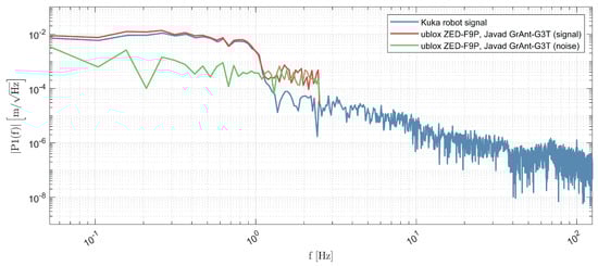
Figure 11.
Session 1: one-sided amplitude spectral density of the GNSS height component of the dynamic test: robot ground truth (blue line), GNSS dynamic signal from the u-blox receiver (red line), and pre-event GNSS noise (green line).
Figure S4 shows the amplitude spectral density for the static kinematic tests of the north component for the RAIL experiment (u-blox F9P logger, u-blox ANN-MB antenna, 1 Hz sampling, 0.5 Hz Nyquist frequency). This illustration gives an impression of the spectral characteristics of the real-time PPP GNSS noise. As indicated by the fitted trend function (red line), the errors approximately follow a power-law noise process, with a slope of approximately −1.9. This indicates that the noise is close to random-walk process (slope of −2) [66]. Such noise characteristics are still the hindering factor in obtaining (sub)millimeter-level for the detection of displacements from GNSS data (e.g., Williams et al. [67], Bos et al. [68], Kuhlmann [69]), and results from unmodelled errors, such as multipath or residual tropospheric effects.
3.2. Session 2—PPP-Wizard Float Solutions, raPPPid Float and Fixed Solutions
This second measurement session was motivated by two aspects: first, we wanted to check the repeatability of precision with the equipment used in the first session, and secondly, we wanted to test the new ASANT antenna.
A central question is, how the ASANT antenna compares to the JAVAD GrAnt antenna, since it comes at a fraction of costs. Firstly, the recorded multi-GNSS data of this session were again processed with PPP-Wizard, generating a PPP float solution. Figure 12 shows the results for the various instrumental setups, starting with the low-cost moving to higher-grade equipment. Regarding the RAIL and the STA1 stations with the u-blox-only and JAVAD-only equipment (plot (a) and plot (d)), the precision obtained for the first sessions can be confirmed—the precision of the geodetic-grade equipment in plot (a) is by approx. a factor of two better than for the u-blox setup in plot (d). Again, the combination of the F9P logger and the ANN-MB antenna reaches sub-decimeter precision. Plots (b) and (c) show the results with the ASANT antenna. Again, it can be seen that low-cost equipment reaches the same level of precision as the geodetic-grade equipment. When comparing plot (c) and (d) it is also noticeable that for the case of the JAVAD receiver, both the ASANT and the JAVAD antenna perform almost identical in terms of noise magnitude and noise shape.

Figure 12.
Session 2: results for the kinematic displacements obtained from the static experiments—ambiguity-float solutions computed with PPP-Wizard.
For comparison purposes we also computed ambiguity-float solutions with raPPPid, for the case of u-blox F9P + ASANT, JAVAD receiver + ASANT and JAVAD receiver + GrAnt. The results are shown in Figure 13. Compared to the PPP-Wizard float solutions presented in Figure 12, these show better results for the horizontal components, and slightly worse results for the Up component. However, the quality is comparable. It is also noticeable that, besides small differences in remaining outliers, plots (a) to (c) of Figure 13 show a high correlation in noise magnitude and shape as well. This indicates, that both the u-blox and the JAVAD receiver, as well as the ASANT and GrAnt antenna have a very similar performance.

Figure 13.
Session 2: results for the kinematic displacements obtained from the static experiments—ambiguity-float solution computed with raPPPid.
Finally, Figure 14 presents the PPP-AR results (calculated with raPPPid) of the corresponding float solutions presented in Figure 12. Likewise as for the float ambiguity case, Figure 14 shows the results for the u-blox F9P logger + ASANT antenna (plot (a)), JAVAD receiver + ASANT antenna (plot (b)), and JAVAD receiver + JAVAD antenna (plot (c)). We could not satisfactorily solve integer ambiguities for the case of the u-blox F9P logger with the u-blox ANN-MB antenna, so there are no results shown here. For the combination of the u-blox + ASANT (plot (a)), the precision could be significantly increased by the integer fixing of the ambiguities (approx. by 10% to 40%, component-wise). This is the configuration, where the highest improvement could be achieved by the AR. For the case of JAVAD SIGMA + ASANT, the improvement by the AR was up to 36%. The results for the JAVAD + GrAnt combination (plot (c)) show a slight worsening in the horizontal components compared to the float solutions. We observe a lower carrier signal-to-noise (SNR) ratio for the configuration in plot (c), which can cause these issues. This is briefly discussed in the supplementary (Figure S5). Note that no Galileo ambiguities were fixed for the case of the JAVAD receiver, so these results are likely to be improved by a Galileo AR fixing. For both, the raPPPid float and fixed solutions there are still few outliers present in the results. These are caused by wrongly fixed ambiguities, and gross measurement errors. Overall, we observe a comparable performance of both, the ASANT antenna, as well as the u-blox F9P receiver when being compared to the geodetic equipment. The quality of the solutions of sessions 1 and 2 is further discussed in Section 3.3.

Figure 14.
Session 2: results for the kinematic displacements obtained from the static experiments—ambiguity-fixed solutions computed with raPPPid.
Figure 15 shows the PPP-AR results for the u-blox F9P + ASANT antenna without applying PCO/PCV corrections. The topocentric transformation is carried out regarding the so-obtained biased reference coordinates (plot (a)). For this case, the precision of the displacements is not affected by the missing PCVs for this antenna. Plot (b) shows the results for the identical configuration (no PCOs/PCVs corrected) but with the topocentric correction carried out regarding the unbiased reference coordinates (with PCOs/PCVs corrected). As a consequence of the missing PCOs/PCVs, the height coordinate gets biased by around 5 cm, which significantly degrades the accuracy of the results. Similar behavior was also reported by Ahmed et al. [50] for the tropospheric estimates (which is highly correlated with the height) with PPP-Wizard. This can be mostly attributed to the missing PCOs, which make up several centimeters for this antenna; however, the effect of missing PCVs can also cause biases of a centimeter or more [70].
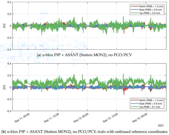
Figure 15.
Session 2: results for the kinematic displacements obtained from the static experiments: PPP-AR solutions computed with raPPPid with/without PCO/PCV corrections. Top plot: no PCOs/PCVs corrected. The topocentric coordinates were computed with the biased reference coordinates. Bottom plot: no PCOs/PCVs corrected. The topocentric coordinates were computed with the unbiased reference coordinates.
For the case of u-blox F9P + ASANT we also computed an ambiguity-float solution with Galileo-and-Glonass-only. The results are shown in Figure S6. RMS values are about 2–4 cm for the horizontal (component-wise) and around 6 cm for the vertical. This demonstrates that high-precision, real-time PPP with low-cost equipment is also possible without considering GPS observations.
3.3. Discussion—Sessions 1 and 2
Table 3 summarizes the RMS values for all ambiguity-float solutions for the static-kinematic experiments of sessions 1 and 2. On average, the obtained precision was 2.1 cm, 1.7 cm and 4.2 cm for the North, East and Up component, respectively. Table 4 shows the RMS values for the ambiguity-fixed solutions for the static-kinematic experiments of session 2. On average, the obtained precision was 1.5 cm, 1.2 cm and 3.6 cm. The relative improvement in precision resulting from the ambiguity fixing is about 30% for the horizontal components, and around 15% for the Up component, respectively.
Table 3.
RMS values for ambiguity float solutions of sessions 1 and 2 (in centimeters).
Table 4.
RMS values for ambiguity fixed solutions of session 2 (in centimeters).
Referring to Table 4, the average ambiguity fixing success rate for u-blox + ASANT is 87% (GPS) and 82% (Galileo), 93% for JAVAD + ASANT (GPS), and 91% for JAVAD + GrAnt (GPS). As mentioned earlier, the Galileo ambiguities could not be fixed for the case of the JAVAD receiver, since satellite bias products were not available for the Galileo signals tracked by this receiver—by fixing the Galileo ambiguities, additional improvements can be expected for the JAVAD-case. As a consequence of raPPPid’s real-time estimation process of the AR solutions (epoch-by-epoch least-squares, with a up-weighting of ambiguity-fixed observations), the design matrix might not be set-up optimally, which then affects the detectability of outliers, and can amplify the effect of high observation noise on certain satellites, when single-GNSS-only AR is considered. Thus multipath signals can also have a higher impact on the solutions, as it might be the case for Figure 14, plot (c). Nevertheless, the results of the raPPPid solutions are of considerable quality, and in terms of precision the best results were obtained for the JAVAD + ASANT combination for the raPPPid float and AR solutions. With raPPPid, the ambiguities were fixed for 99.94%, 99.30% and 99.29% of the epochs for the u-blox + ASANT, the JAVAD + ASANT and the JAVAD + GrAnt case, respectively. It should be one more strengthened that amongst the various PPP solutions shown in Figure 12 and Figure 13, the results of the different instrumentation setups lead to very similar results. This indicates that both the geodetic-grade and the low-cost receivers, as well as the geodetic-grade and (helical-type) low-cost antennas perform quite similar.
3.4. Session 3—Point Perfect PPP-RTK Solutions
This section shows the results obtained for the u-blox PointPerfect PPP-RTK service (with fixed ambiguities) for sub-session 2 (27 April 2022, Figure 16) and sub-session 4 (4 May 2022, Figure 17). Plots (a) show the results for the u-blox F9P logger + ANN-MB antenna, and plots (b) show the results for the u-blox F9P + ASANT antenna. Additionally, the Figures S7 and S8 show the coordinate series for the other two sub-sessions (1 and 3).

Figure 16.
Session 3—sub-session 2: results for the kinematic displacements obtained from the static experiments—PPP-RTK solution obtained with PointPerfect.

Figure 17.
Session 3—sub-session 4: results for the kinematic displacements obtained from the static experiments—PPP-RTK solution obtained with PointPerfect.
It gets clear that the horizontal precision is at the level of several centimeters, and around 10 cm for the height component. This is a factor two worse than the precision achieved with PPP-Wizard and raPPPid. However, the achieved precision is in agreement with the formal errors specified by u-blox. Gaps in the coordinate series correspond to float-only solutions, which were removed. Notably, thanks to the additional corrections of the atmosphere, ambiguities can be solved faster than with PPP-Wizard or raPPPid. For our tests, it typically took several tens of seconds (cold-start) until the ambiguities were solved. This is basically in accordance with the specifications of u-blox with initialization times less than 30 s. In terms of absolute coordinate accuracy, the missing PCOs/PCVs still can bias the result on centimeter-level.
4. Conclusions
In this work, we analyzed the performance of the u-blox ZED-F9P GNSS module for kinematic real-time PPP applications. It was demonstrated that these low-cost GNSS devices are suitable for high-rate geomonitoring applications, such as GNSS seismology, which has centimeter-level precision requirements. We also investigated the performance of the F9P in combination with different antennas, i.e., the low-cost u-blox ANN-MB patch antenna, the low-cost Ardusimple helical-type ASANT antenna, and the geodetic medium-grade helical-type JAVAD GrAnt3 antenna. Except for the ANN-MB patch antenna, the results obtained for the low-cost and geodetic-grade equipment showed a very similar performance. Even with the ANN-MB patch antenna, precisions at the sub-decimeter level could be achieved, component-wise.
Based on static experiments of three sessions, processed in kinematic mode, we obtained a precision of few centimeters in the horizontal, and of about 3 to 10 cm in the height component. The first two sessions were processed using state-of-the-art real-time PPP software (PPPWizard and raPPPid)—we obtained an average precision of 2.1, 1.7 and 4.2 cm for the ambiguity-float solutions, and 1.5, 1.2 and 3.6 cm for the fixed solutions, respectively. Concerning the low-cost aspect, the most promising results were achieved with the u-blox F9P + ASANT antenna. By applying AR, the results even reach the centimeter-level for this case. Based on experimental tests with a robot arm, the u-blox F9P has demonstrated its capability to resolve seismic strong-motion signals at a level of detail very similar to that of geodetic-grade receivers. In terms of absolute accuracy, it was shown that without correcting for PCOs/PCVs a significant bias in the height component is introduced (i.e., around 5 cm for the ASANT antenna). Besides navigational aspects, the recently launched u-blox PPP-RTK service offers also very interesting perspectives for geomonitoring applications, since—thanks to the additional corrections—ambiguities can be fixed very fast. Furthermore, users directly obtain high-precision coordinates with no intermediate processing steps, which makes it an interesting instrumentation for the geoscience community as well. In view of kinematic applications, further experiments should address the value of receiver antenna corrections for the ANN-MB patch antenna. Depending on the antenna type, missing PCVs may degrade accuracy up to the level of few centimeters [60,70]. It is also envisaged to further optimize the recursive multi-GNSS real-time parameter estimation methods for the AR processing of the raPPPid software (e.g., Teunissen [71]), so that the effect of observation errors can be further reduced. However, even for low-cost equipment, multi-GNSS float-ambiguity solutions can already provide precision at the centimeter-level—by using the raPPPid software developed at TU Vienna we could demonstrate that single- and multi-GNSS PPP-AR can improve the coordinate results by up to 40% or more.
We conclude, that in terms of obtainable accuracy and precision, the results of u-blox F9P + ASANT antenna are comparable to those obtained with geodetic-grade equipment. Therefore, it can be stated that the tested low-cost equipment meets the demands for GNSS high-rate monitoring applications, such as EEW. Consequently, the combination of a u-blox F9P with low-cost helical-type antennas is a very promising way to densify existing GNSS monitoring networks, and it comes at a fraction of the costs of high-grade GNSS equipment. Finally, we conclude that the tested devices can be used to resolve dynamic ground movements at the centimeter level, which is a requirement for strong-motion seismology and EEW (e.g., Ruhl et al. [61], Melgar et al. [62]).
Supplementary Materials
The following supporting information can be downloaded at: https://www.mdpi.com/article/10.3390/rs14205100/s1, Figure S1: Session 1: results for the kinematic displacements obtained from the static experiments—ambiguity-float solutions computed with PPP-Wizard; Figure S2: The ground truth of the synthetic seismic strong-motion signal; Figure S3: Results for the dynamic tests with the seismic strong-motion waveforms (JAVAD receiver and JAVAD antenna); Figure S4: Session 1: one-sided amplitude spectral density of the north component for the static kinematic test; Figure S5: Session 2: Carrier signal-to-noise (SNR) ratio for GPS L1 frequency; Figure S6: Session 2: results for the kinematic displacements obtained from the static experiments—ambiguity-float solution computed with raPPPid (Galileo and Glonass); Figure S7: Session 3—sub-session 1: results for the kinematic displacements obtained from the static experiments —PPP-RTK solution obtained with PointPerfect; Figure S8: Session 3—sub-session 3: results for the kinematic displacements obtained from the static experiments: PPP-RTK solution obtained with PointPerfect.
Author Contributions
Conceptualization, R.H., R.S. and M.R.; methodology, R.H., R.S., M.F.G. and J.C.; software, R.H., R.S., M.F.G., I.D.H.P. and E.V.; validation, R.H., R.S., M.F.G., I.D.H.P. and E.V.; formal analysis, R.H., R.S., M.F.G., I.D.H.P., E.V. and Y.R.; writing—original draft preparation, R.H., R.S. and M.F.G.; resources, R.H., R.S. and M.F.G.; investigation, R.H., J.C. and M.R.; supervision, R.H. and M.R.; writing—review and editing, R.H., J.C. and M.R. All authors have read and agreed to the published version of the manuscript.
Funding
This research received no external funding.
Institutional Review Board Statement
Not applicable.
Informed Consent Statement
Not applicable.
Data Availability Statement
Data can be made available on request.
Acknowledgments
We want to thank the three anonymous reviewers for their valuable comments.
Conflicts of Interest
The authors declare no conflict of interest.
References
- Montenbruck, O.; Steigenberger, P.; Hauschild, A. Comparing the ‘Big 4’-A User’s View on GNSS Performance. In Proceedings of the 2020 IEEE/ION Position, Location and Navigation Symposium (PLANS), Portland, OR, USA, 20–23 April 2020; pp. 407–418. [Google Scholar]
- Teunissen, P.; Montenbruck, O. Springer Handbook of Global Navigation Satellite Systems; Springer: Berlin/Heidelberg, Germany, 2017. [Google Scholar]
- Alkan, R.M.; Erol, S.; İlçi, V.; Ozulu, İ.M. Comparative analysis of real-time kinematic and PPP techniques in dynamic environment. Measurement 2020, 163, 107995. [Google Scholar] [CrossRef]
- Chen, J.; Li, H.; Wu, B.; Zhang, Y.; Wang, J.; Hu, C. Performance of real-time precise point positioning. Mar. Geod. 2013, 36, 98–108. [Google Scholar] [CrossRef]
- Hadas, T. GNSS-Warp software for real-time precise point positioning. Artif. Satell. 2015, 50, 59. [Google Scholar]
- Wang, L.; Li, Z.; Ge, M.; Neitzel, F.; Wang, Z.; Yuan, H. Validation and assessment of multi-GNSS real-time precise point positioning in simulated kinematic mode using IGS real-time service. Remote Sens. 2018, 10, 337. [Google Scholar] [CrossRef]
- Elsobeiey, M.; Al-Harbi, S. Performance of real-time Precise Point Positioning using IGS real-time service. GPS Solut. 2016, 20, 565–571. [Google Scholar] [CrossRef]
- Kouba, J.; Héroux, P. Precise point positioning using IGS orbit and clock products. GPS Solut. 2001, 5, 12–28. [Google Scholar] [CrossRef]
- Zumberge, J.; Heflin, M.; Jefferson, D.; Watkins, M.; Webb, F.H. Precise point positioning for the efficient and robust analysis of GPS data from large networks. J. Geophys. Res. Solid Earth 1997, 102, 5005–5017. [Google Scholar] [CrossRef]
- Yu, X.; Gao, J. Kinematic precise point positioning using multi-constellation global navigation satellite system (GNSS) observations. ISPRS Int. J. Geo-Inf. 2017, 6, 6. [Google Scholar] [CrossRef]
- Leandro, R.; Landau, H.; Nitschke, M.; Glocker, M.; Seeger, S.; Chen, X.; Deking, A.; BenTahar, M.; Zhang, F.; Ferguson, K.; et al. RTX positioning: The next generation of cm-accurate real-time GNSS positioning. In Proceedings of the 24th International Technical Meeting of the Satellite Division of the Institute of Navigation (ION GNSS 2011), Portland, OR, USA, 19–23 September 2011; pp. 1460–1475. [Google Scholar]
- Wubbena, G.; Schmitz, M.; Bagge, A. PPP-RTK: Precise point positioning using state-space representation in RTK networks. In Proceedings of the 18th international technical meeting of the satellite division of the Institute of navigation (ION GNSS 2005), Fort Worth, TX, USA, 25–28 September 2005; pp. 2584–2594. [Google Scholar]
- Teunissen, P.; Khodabandeh, A. Review and principles of PPP-RTK methods. J. Geod. 2015, 89, 217–240. [Google Scholar] [CrossRef]
- Li, X.; Zhang, X.; Ge, M. Regional reference network augmented precise point positioning for instantaneous ambiguity resolution. J. Geod. 2011, 85, 151–158. [Google Scholar] [CrossRef]
- Glaner, M.; Weber, R. PPP with integer ambiguity resolution for GPS and Galileo using satellite products from different analysis centers. GPS Solut. 2021, 25, 1–13. [Google Scholar]
- Laurichesse, D.; Mercier, F.; Berthias, J.P.; Broca, P.; Cerri, L. Integer ambiguity resolution on undifferenced GPS phase measurements and its application to PPP and satellite precise orbit determination. Navigation 2009, 56, 135–149. [Google Scholar] [CrossRef]
- Ge, M.; Gendt, G.; Rothacher, M.A.; Shi, C.; Liu, J. Resolution of GPS carrier-phase ambiguities in precise point positioning (PPP) with daily observations. J. Geod. 2008, 82, 389–399. [Google Scholar] [CrossRef]
- Banville, S.; Geng, J.; Loyer, S.; Schaer, S.; Springer, T.; Strasser, S. On the interoperability of IGS products for precise point positioning with ambiguity resolution. J. Geod. 2020, 94, 1–15. [Google Scholar] [CrossRef]
- Tsakiri, M.; Sioulis, A.; Piniotis, G. The use of low-cost, single-frequency GNSS receivers in mapping surveys. Surv. Rev. 2018, 50, 46–56. [Google Scholar] [CrossRef]
- Lu, L.; Ma, L.; Wu, T.; Chen, X. Performance analysis of positioning solution using low-cost single-frequency u-blox receiver based on baseline length constraint. Sensors 2019, 19, 4352. [Google Scholar] [CrossRef]
- Kenner, R.; Pruessner, L.; Beutel, J.; Limpach, P.; Phillips, M. How rock glacier hydrology, deformation velocities and ground temperatures interact: Examples from the Swiss Alps. Permafr. Periglac. Process. 2020, 31, 3–14. [Google Scholar] [CrossRef]
- Cina, A.; Piras, M. Performance of low-cost GNSS receiver for landslides monitoring: Test and results. Geomat. Nat. Hazards Risk 2015, 6, 497–514. [Google Scholar] [CrossRef]
- Tsakiri, M.; Sioulis, A.; Piniotis, G. Compliance of low-cost, single-frequency GNSS receivers to standards consistent with ISO for control surveying. Int. J. Metrol. Qual. Eng. 2017, 8, 11. [Google Scholar] [CrossRef]
- Garrido-Carretero, M.S.; Borque-Arancón, M.J.; Ruiz-Armenteros, A.M.; Moreno-Guerrero, R.; Gil-Cruz, A.J. Low-cost GNSS receiver in RTK positioning under the standard ISO-17123-8: A feasible option in geomatics. Measurement 2019, 137, 168–178. [Google Scholar] [CrossRef]
- Odolinski, R.; Teunissen, P.J. Single-frequency, dual-GNSS versus dual-frequency, single-GNSS: A low-cost and high-grade receivers GPS-BDS RTK analysis. J. Geod. 2016, 90, 1255–1278. [Google Scholar] [CrossRef]
- Hamza, V.; Stopar, B.; Sterle, O. Testing the performance of multi-frequency low-cost gnss receivers and antennas. Sensors 2021, 21, 2029. [Google Scholar] [CrossRef]
- Takasu, T.; Yasuda, A. Development of the low-cost RTK-GPS receiver with an open source program package RTKLIB. In Proceedings of the International Symposium on GPS/GNSS. International Convention Center, Jeju, Korea, 12–17 July 2009; Volume 1. [Google Scholar]
- Hamza, V.; Stopar, B.; Ambrožič, T.; Sterle, O. Performance Evaluation of Low-Cost Multi-Frequency GNSS Receivers and Antennas for Displacement Detection. Appl. Sci. 2021, 11, 6666. [Google Scholar] [CrossRef]
- Tunini, L.; Zuliani, D.; Magrin, A. Applicability of Cost-Effective GNSS Sensors for Crustal Deformation Studies. Sensors 2022, 22, 350. [Google Scholar] [CrossRef]
- Janos, D.; Kuras, P.; Ortyl, Ł. Evaluation of Low-Cost RTK GNSS Receiver in Motion under Demanding Conditions. Measurement 2022, 201, 111647. [Google Scholar] [CrossRef]
- Wielgocka, N.; Hadas, T.; Kaczmarek, A.; Marut, G. Feasibility of using low-cost dual-frequency gnss receivers for land surveying. Sensors 2021, 21, 1956. [Google Scholar] [CrossRef]
- Paziewski, J. Multi-constellation single-frequency ionospheric-free precise point positioning with low-cost receivers. GPS Solut. 2022, 26, 1–11. [Google Scholar] [CrossRef]
- Krietemeyer, A.; van der Marel, H.; van de Giesen, N.; ten Veldhuis, M.C. High quality zenith tropospheric delay estimation using a low-cost dual-frequency receiver and relative antenna calibration. Remote Sens. 2020, 12, 1393. [Google Scholar] [CrossRef]
- Nie, Z.; Liu, F.; Gao, Y. Real-time precise point positioning with a low-cost dual-frequency GNSS device. GPS Solut. 2020, 24, 1–11. [Google Scholar] [CrossRef]
- Bock, Y.; Wdowinski, S. GNSS Geodesy in Geophysics, Natural Hazards, Climate, and the Environment. In Position, Navigation, and Timing Technologies in the 21st Century: Integrated Satellite Navigation, Sensor Systems, and Civil Applications; John Wiley & Sons: Hoboken, NJ, USA, 2020; Volume 1, pp. 741–820. [Google Scholar]
- Shen, N.; Chen, L.; Liu, J.; Wang, L.; Tao, T.; Wu, D.; Chen, R. A Review of Global Navigation Satellite System (GNSS)-based Dynamic Monitoring Technologies for Structural Health Monitoring. Remote Sens. 2019, 11, 1001. [Google Scholar] [CrossRef]
- Bock, Y.; Melgar, D.; Crowell, B.W. Real-time strong-motion broadband displacements from collocated GPS and accelerometers. Bull. Seismol. Soc. Am. 2011, 101, 2904–2925. [Google Scholar] [CrossRef]
- Murray, J.R.; Crowell, B.W.; Grapenthin, R.; Hodgkinson, K.; Langbein, J.O.; Melbourne, T.; Melgar, D.; Minson, S.E.; Schmidt, D.A. Development of a geodetic component for the US West Coast earthquake early warning system. Seismol. Res. Lett. 2018, 89, 2322–2336. [Google Scholar] [CrossRef]
- Dahmen, N.; Hohensinn, R.; Clinton, J. Comparison and Combination of GNSS and Strong-Motion Observations: A Case Study of the 2016 Mw 7.0 Kumamoto Earthquake. Bull. Seismol. Soc. Am. 2020, 110, 2647–2660. [Google Scholar] [CrossRef]
- Ohta, Y.; Kobayashi, T.; Tsushima, H.; Miura, S.; Hino, R.; Takasu, T.; Fujimoto, H.; Iinuma, T.; Tachibana, K.; Demachi, T.; et al. Quasi real-time fault model estimation for near-field tsunami forecasting based on RTK-GPS analysis: Application to the 2011 Tohoku-Oki earthquake (Mw 9.0). J. Geophys. Res. Solid Earth 2012, 117, B02311. [Google Scholar] [CrossRef]
- Limpach, P.; Geiger, A.; Raetzo, H. GNSS for deformation and geohazard monitoring in the Swiss Alps. In Proceedings of the 3rd Joint International Symposium on Deformation Monitoring (JISDM 2016), Vienna, Austria, 30 March–1 April 2016; Volume 30. [Google Scholar]
- Melgar, D.; Melbourne, T.I.; Crowell, B.W.; Geng, J.; Szeliga, W.; Scrivner, C.; Santillan, M.; Goldberg, D.E. Real-time high-rate GNSS displacements: Performance demonstration during the 2019 Ridgecrest, California, earthquakes. Seismol. Res. Lett. 2020, 91, 1943–1951. [Google Scholar] [CrossRef]
- Ruhl, C.; Melgar, D.; Grapenthin, R.; Allen, R. The value of real-time GNSS to earthquake early warning. Geophys. Res. Lett. 2017, 44, 8311–8319. [Google Scholar] [CrossRef]
- Clinton, J.; Geiger, A.; Häberling, S.; Haslinger, F.; Rothacher, M.; Wiget, A.; Wild, U. The future of national GNSS geomonitoring infrastructures in Switzerland. In Geodätisch-geophysikalische Arbeiten in der Schweiz; Schweizerische Geodätische Kommision: Zurich, Switzerland, 2017. [Google Scholar]
- Laurichesse, D. The CNES Real-time PPP with undifferenced integer ambiguity resolution demonstrator. In Proceedings of the 24th International Technical Meeting of The Satellite Division of the Institute of Navigation (ION GNSS 2011), Portland, OR, USA, 19–23 September 2011; pp. 654–662. [Google Scholar]
- u-blox. PointPerfect Product Summary. 2011. Available online: https://content.u-blox.com/sites/default/files/PointPerfect_ProductSummary_UBX-21024758.pdf (accessed on 30 June 2022).
- Rossi, Y.; Tatsis, K.; Awadaljeed, M.; Arbogast, K.; Chatzi, E.; Rothacher, M.; Clinton, J. Kalman filter-based fusion of collocated acceleration, GNSS and rotation data for 6C motion tracking. Sensors 2021, 21, 1543. [Google Scholar] [CrossRef]
- u-blox. u-blox Point Perfect GNSS Augmentation Service. 2022. Available online: https://www.u-blox.com/en/product/pointperfect (accessed on 11 June 2022).
- Laurichesse, D.; Privat, A. An open-source PPP client implementation for the CNES PPP-WIZARD demonstrator. In Proceedings of the 28th International Technical Meeting of the Satellite Division of The Institute of Navigation (ION GNSS+ 2015), Dana Point, CA, USA, 26–28 January 2015; pp. 2780–2789. [Google Scholar]
- Ahmed, F.; Vaclavovic, P.; Teferle, F.N.; Douša, J.; Bingley, R.; Laurichesse, D. Comparative analysis of real-time precise point positioning zenith total delay estimates. GPS Solut. 2016, 20, 187–199. [Google Scholar] [CrossRef]
- Kazmierski, K.; Sośnica, K.; Hadas, T. Quality assessment of multi-GNSS orbits and clocks for real-time precise point positioning. GPS Solut. 2018, 22, 1–12. [Google Scholar] [CrossRef]
- Boisits, J.; Glaner, M.; Weber, R. Regiomontan: A regional high precision ionosphere delay model and its application in precise point positioning. Sensors 2020, 20, 2845. [Google Scholar] [CrossRef]
- Landskron, D.; Böhm, J. VMF3/GPT3: Refined discrete and empirical troposphere mapping functions. J. Geod. 2018, 92, 349–360. [Google Scholar] [CrossRef]
- Landskron, D.; Böhm, J. Refined discrete and empirical horizontal gradients in VLBI analysis. J. Geod. 2018, 92, 1387–1399. [Google Scholar] [CrossRef]
- Teunissen, P.J.G. The least-squares ambiguity decorrelation adjustment: A method for fast GPS integer ambiguity estimation. J. Geod. 1995, 70, 65–82. [Google Scholar] [CrossRef]
- Mervart, L.; Lukes, Z.; Rocken, C.; Iwabuchi, T. Precise point positioning with ambiguity resolution in real-time. In Proceedings of the 21st International Technical Meeting of the Satellite Division of the Institute of Navigation (ION GNSS 2008), Savannah, GA, USA, 16–19 September 2008; pp. 397–405. [Google Scholar]
- Zhang, B.; Chen, Y.; Yuan, Y. PPP-RTK based on undifferenced and uncombined observations: Theoretical and practical aspects. J. Geod. 2019, 93, 1011–1024. [Google Scholar] [CrossRef]
- Odijk, D.; Teunissen, P.J.; Zhang, B. Single-frequency integer ambiguity resolution enabled GPS precise point positioning. J. Surv. Eng. 2012, 138, 193–202. [Google Scholar] [CrossRef]
- Psychas, D.; Verhagen, S. Real-time PPP-RTK performance analysis using ionospheric corrections from multi-scale network configurations. Sensors 2020, 20, 3012. [Google Scholar] [CrossRef]
- Banville, S.; Tang, H. Antenna rotation and its effects on kinematic precise point positioning. In Proceedings of the 23rd International Technical Meeting of The Satellite Division of the Institute of Navigation (ION GNSS 2010), Portland, OR, USA, 21–24 September 2010; pp. 2545–2552. [Google Scholar]
- Ruhl, C.J.; Melgar, D.; Geng, J.; Goldberg, D.E.; Crowell, B.W.; Allen, R.M.; Bock, Y.; Barrientos, S.; Riquelme, S.; Baez, J.C.; et al. A global database of strong-motion displacement GNSS recordings and an example application to PGD scaling. Seismol. Res. Lett. 2019, 90, 271–279. [Google Scholar] [CrossRef]
- Melgar, D.; Crowell, B.W.; Melbourne, T.I.; Szeliga, W.; Santillan, M.; Scrivner, C. Noise characteristics of operational real-time high-rate GNSS positions in a large aperture network. J. Geophys. Res. Solid Earth 2020, 125, e2019JB019197. [Google Scholar] [CrossRef]
- Häberling, S. Theoretical and Practical Aspects of High-Rate GNSS Geodetic Observations. Ph.D. Thesis, ETH-Zürich, Zürich, Swiss, 2015. [Google Scholar]
- Michel, C.; Kelevitz, K.; Houlié, N.; Edwards, B.; Psimoulis, P.; Su, Z.; Clinton, J.; Giardini, D. The potential of high-rate GPS for strong ground motion assessment. Bull. Seismol. Soc. Am. 2017, 107, 1849–1859. [Google Scholar] [CrossRef]
- Häberling, S.; Rothacher, M.; Zhang, Y.; Clinton, J.; Geiger, A. Assessment of high-rate GPS using a single-axis shake table. J. Geod. 2015, 89, 697–709. [Google Scholar] [CrossRef]
- Montillet, J.P.; Bos, M.S. Geodetic Time Series Analysis in Earth Sciences; Springer: Berlin/Heidelberg, Germany, 2019. [Google Scholar]
- Williams, S.D.; Bock, Y.; Fang, P.; Jamason, P.; Nikolaidis, R.M.; Prawirodirdjo, L.; Miller, M.; Johnson, D.J. Error analysis of continuous GPS position time series. J. Geophys. Res. Solid Earth 2004, 109, B03412. [Google Scholar] [CrossRef]
- Bos, M.; Fernandes, R.; Williams, S.; Bastos, L. Fast error analysis of continuous GPS observations. J. Geod. 2008, 82, 157–166. [Google Scholar] [CrossRef]
- Kuhlmann, H. Kalman-filtering with coloured measurement noise for deformation analysis. In Proceedings of the 11th FIG Symposium on Deformation Measurements, Santorini, Greece, 25–28 May 2003. [Google Scholar]
- Schmid, R.; Rothacher, M.; Thaller, D.; Steigenberger, P. Absolute phase center corrections of satellite and receiver antennas. GPS Solut. 2005, 9, 283–293. [Google Scholar] [CrossRef]
- Teunissen, P.J. Batch and Recursive Model Validation. In Springer Handbook of Global Navigation Satellite Systems; Teunissen, P.J., Montenbruck, O., Eds.; Springer Handbooks; Springer: Cham, Switzerland, 2017; pp. 687–720. [Google Scholar]
Publisher’s Note: MDPI stays neutral with regard to jurisdictional claims in published maps and institutional affiliations. |
© 2022 by the authors. Licensee MDPI, Basel, Switzerland. This article is an open access article distributed under the terms and conditions of the Creative Commons Attribution (CC BY) license (https://creativecommons.org/licenses/by/4.0/).