Article

Revisiting Ice Flux and Mass Balance of the Lambert Glacier–Amery Ice Shelf System Using Multi-Remote-Sensing Datasets, East Antarctica

1
Key Laboratory of Fishery Information, Ministry of Agriculture, College of Information Technology, Shanghai Ocean University, Shanghai 201306, China
2
Key Laboratory of Polar Science, MNR, Polar Research Institute of China, Shanghai 200136, China
3
School of Oceanography, Shanghai Jiao Tong University, Shanghai 200030, China
4
College of Surveying and Geo-Informatics, Tongji University, Shanghai 200092, China
*
Author to whom correspondence should be addressed.
Remote Sens. 2022, 14(2), 391; https://doi.org/10.3390/rs14020391
Submission received: 19 November 2021 / Revised: 12 January 2022 / Accepted: 13 January 2022 / Published: 14 January 2022
(This article belongs to the Special Issue Remote Sensing of Polar Regions)

Abstract

:
Due to rapid global warming, the relationship between the mass loss of the Antarctic ice sheet and rising sea levels are attracting widespread attention. The Lambert–Amery glacial system is the largest drainage system in East Antarctica, and its mass balance has an important influence on the stability of the Antarctic ice sheet. In this paper, the recent ice flux in the Lambert Glacier of the Lambert–Amery system was systematically analyzed based on recently updated remote sensing data. According to Landsat-8 ice velocity data from 2018 to April 2019 and the updated Bedmachine v2 ice thickness dataset in 2021, the contribution of ice flux approximately 140 km downstream from Dome A in the Lambert Glacier area to downstream from the glacier is 8.5 ± 1.9   Gt · a 1 , and the ice flux in the middle of the convergence region is 18.9 ± 2.9   Gt · a 1 . The ice mass input into the Amery ice shelf through the grounding line of the whole glacier is 19.9 ± 1.3   Gt · a 1 . The ice flux output from the mainstream area of the grounding line is 19.3 ± 1.0   Gt · a 1 . Using the annual SMB data of the regional atmospheric climate model (RACMO v2.3) as the quality input, the mass balance of the upper, middle, and lower reaches of the Lambert Glacier was analyzed. The results show that recent positive accumulation appears in the middle region of the glacier (about 74–78°S, 67–85°E) and the net accumulation of the whole glacier is 2.4 ± 3.5   Gt · a 1 . Although the mass balance of the Lambert Glacier continues to show a positive accumulation, and the positive value in the region is decreasing compared with values obtained in early 2000.

1. Introduction

The Antarctic ice sheet (AIS) stores approximately 90% of the world’s ice, with a total volume of approximately 2.65 × 10 7   km 3 . If it were to melt completely, global sea levels would rise by about 57.2 m [1,2]. Satellite measurements show that the mass of the AIS is accelerating and flowing into the Southern Ocean through different drainage systems, a phenomenon that is particularly pronounced in the West Antarctic ice sheet (WAIS) [3,4,5]. The East Antarctic ice sheet (EAIS) has a volume four times greater than the ice reserves of the WAIS, and its potential impact on rising sea levels has attracted extensive attention in recent years [6,7]. The Lambert–Amery system (LAS) is the largest drainage system in EAIS, and covers an area of more than 1.6 × 10 7   km 2 , accounting for 16% of the total area of the EAIS, and its ice reserves account for approximately 10% of the entire AIS. Therefore, this is an important region to study and understand the impact of the EAIS on current and future climate change [8,9,10]. The main components of LAS consist of three glaciers, the Fisher, Mellor, and Lambert Glaciers, collectively known as the Lambert Basin, which converge in the southern Amery ice shelf and flows into the floating ice shelf through the grounding line to become the central flow zone [11]. The Lambert Glacier has the largest output ice flux among the three, which plays an important role in evaluating the mass balance of LAS [12].
Studies on ice flux and surface mass balance (SMB) of LAS have been carried out for decades [2,6,13,14,15]. Allison (1979) calculated the ice flux flowing into the south of the Amery ice shelf by using early measured ice velocity and ice thickness data. Combined with ice and snow accumulation in the upstream region, it was estimated that the net accumulation in the Lambert basin region exceeded 30   Gt · a 1 [12]. In the following 20 years, the estimation of LAS mass balance and the measurement of surface velocity were mainly carried out around the Australian National Antarctic Research Expedition Lambert Glacier Basin (ANARE LGB) traverse. The location of the ANARE LGB traverse is shown in Figure 1. Fricker et al. (2000) calculated the ice flux through the LGB Traverse as 44   Gt · a 1 by using in situ measurement data of ANARE traverse over five seasons from 1989 to 1995, and estimated the net accumulation variation ranged from −15.3   Gt · a 1 to +8.8   Gt · a 1 [16]. At the beginning of the 21st century, with the development of remote sensing technologies such as laser altimeters, interferometric synthetic aperture radars (SAR), and Global Positioning Systems (GPS), the measurement capabilities of Antarctic surface velocity and grounding line positions have been greatly improved [17,18]. Wen et al. (2007) used multi-source satellite elevation data to deduce ice thickness at the upstream grounding line of Amery ice shelf by the method of hydrostatic balance, and then calculated the ice flux output in the Lambert basin by combining ice velocity data of the Modified Antarctic Mapping Mission (MAMM) project in autumn 2000 as 54.0 ± 5.4   Gt · a 1 [2]. Yu et al. (2010) and Wen et al. (2014) used Bedmap data [19] and Bedmap2 data [20], respectively, and combined the ice velocity data of the MAMM project in different periods to obtain values of the ice fluxes of the Lambert basin. Their results were 38.9 ± 2.8   Gt · a 1 and 38.3 ± 2.8   Gt · a 1 [10,15]. The most recent large-scale mass balance estimation in the LAS system was performed by Cui et al. (2020) using in situ measurements from the Chinese National Antarctic Research Expedition (CHINARE) DT traverse, a traverse connecting Dome A to Zhongshan Station, to calculate the total ice flux in the upper Amery eastern basin as 20.9 ± 1.9   Gt · a 1 [6]. The location of the CHINARE DT traverse is shown in the right side image in Figure 1.
However, the aforementioned ice velocity data used to study the ice flux of LAS were obtained over a decade ago. For example, Cui et al. used the measured ice velocity data from 1997 to 2005 and the MAMM ice velocity data from 2007 to 2009, while ice velocity data from other studies were gathered earlier [6]. Meanwhile, the ice thickness data used in previous studies do not match the grid resolution of ice velocity data due to the limitations of previous datasets or field acquisition methods. Moreover, these studies focused on the downstream or upstream ice flux output of some glaciers in LAS and lacked investigations on the movement change of glaciers from upstream to downstream during the same period.
In addition to the study of mass balance on LAS, recent research on the mass balance of AIS was carried out on a larger spatial scale. The Ice Sheet Mass Balance Inter-comparison Exercise (IMBIE) team conducted mass balance assessments on the EAIS, WAIS, and Antarctic Peninsula Ice Sheet (APIS). It was illustrated that the temporal variability of the Antarctic surface mass balance was stable, and the mass loss from AIS was mainly caused by increased solid-ice discharge into the ocean. By combining RACMO2.3, it was concluded that although the EAIS was stable from 1992 to 2017 (5 ± 46   Gt · a 1 ), there was great uncertainty in numerical estimation [21]. Moreover, Rignot et al. re-evaluated the mass balance of the entire AIS from 1979 to 2017 and concluded that the mass balance of the Amery was roughly stable. From the research, the total ice flux in the Amery region from 2007 to 2008 was estimated to be 76.4   Gt · a 1 , and the total SMB was estimated to be 85.7   Gt · a 1 by using the average SMB data of RACMO2.3 from 1978 to 2008 [1]. The results of both studies were restated in the Intergovernmental Panel on Climate Change (IPCC) report of August 2021 [22]. It can be seen that few studies exist on the mass balance of important small-scale glaciers, and the mass balance estimation in the EAIS has remained highly uncertain over the last 30 years. By studying a single important glacier, these uncertainties may be refined.
Figure 1. The location of the study area in Antarctica is indicated by the red box at the top left. Right: The three ice gates Gate 1, Gate 2, and Gate 3 defined in this paper are all represented by black dotted lines, and the starting point and ending points are (A1, A2), (B1, B2), and (C1, C2), respectively. The enlarged view on the black dotted line is a schematic of the ice gate. The orange grounding line is taken from the MOA 2014 Image Map (updated in 2019) [23,24]. The internal red lines were taken from the drainage basins of the 2007–2009 International Polar Years (IPY) program (2017) [25,26]. The background color is the ice velocity from Shen Qiang et al. [27]. The blue and pink dots on ANARE traverse and CHINARE DT traverse represent GPS ice flow monitoring points. Lower left: Gate 3 is created from the grounding line position of the MOA 2014, represented by a dashed red and black line [23,24]. The length of the red line beginning with C1 is thicker than the latter half, indicating the mainstream area on Gate 3. Yellow lines represent the grounding line position of IPY [25,26].
Remotesensing 14 00391 g001
In this paper, the latest updated datasets from remote sensing, airborne geophysical observations, and atmospheric climate models were used to study the changes in the ice movement in the Lambert Glacier from the upstream to the grounding line and to revisit the ice flow flux along different sections of Lambert Glacier. The area is shown by the red line demarcation in Figure 1. The ice velocity data were derived from Landsat-8 (L8) images of Antarctic observations from 2018 to 2019 [27], and the ice thickness was obtained from the recently updated BedMachine v2 dataset [28,29]. Due to the same grid resolution of ice velocity and ice thickness, the redundant interpolation matching operation was avoided, which was helpful in improving the accuracy of the estimated ice flux.

2. Materials and Methods

2.1. Data Sources

Six datasets were used to calculate the ice flux of the Lambert Glacier in East Antarctica from November 2018 to April 2019 and estimate mass balance in the study area, as shown in Table 1. The data included basin delineation, grounding line, ice surface velocity, the ice surface and ground elevation, and ice thickness. The surface ice velocity data were obtained from the Antarctic ice flow map released by Shen Qiang et al., while other datasets were gathered from the NASA Making Earth System Data Records for Use in Research Environments (MEaSUREs) program. For the input term of the mass balance, we used the semi-empirical regional atmospheric climate model (RACMO v2.3) [30] to estimate the surface mass balance (SMB) in the Lambert region. All data products were processed and calculated in the same projection/coordinate system (EPSG: 4326 GCS_WGS_1984/Polar Stereographic). At the same time, the errors of the ice flux and mass balance were quantified according to the statistical theory of error propagation [31].

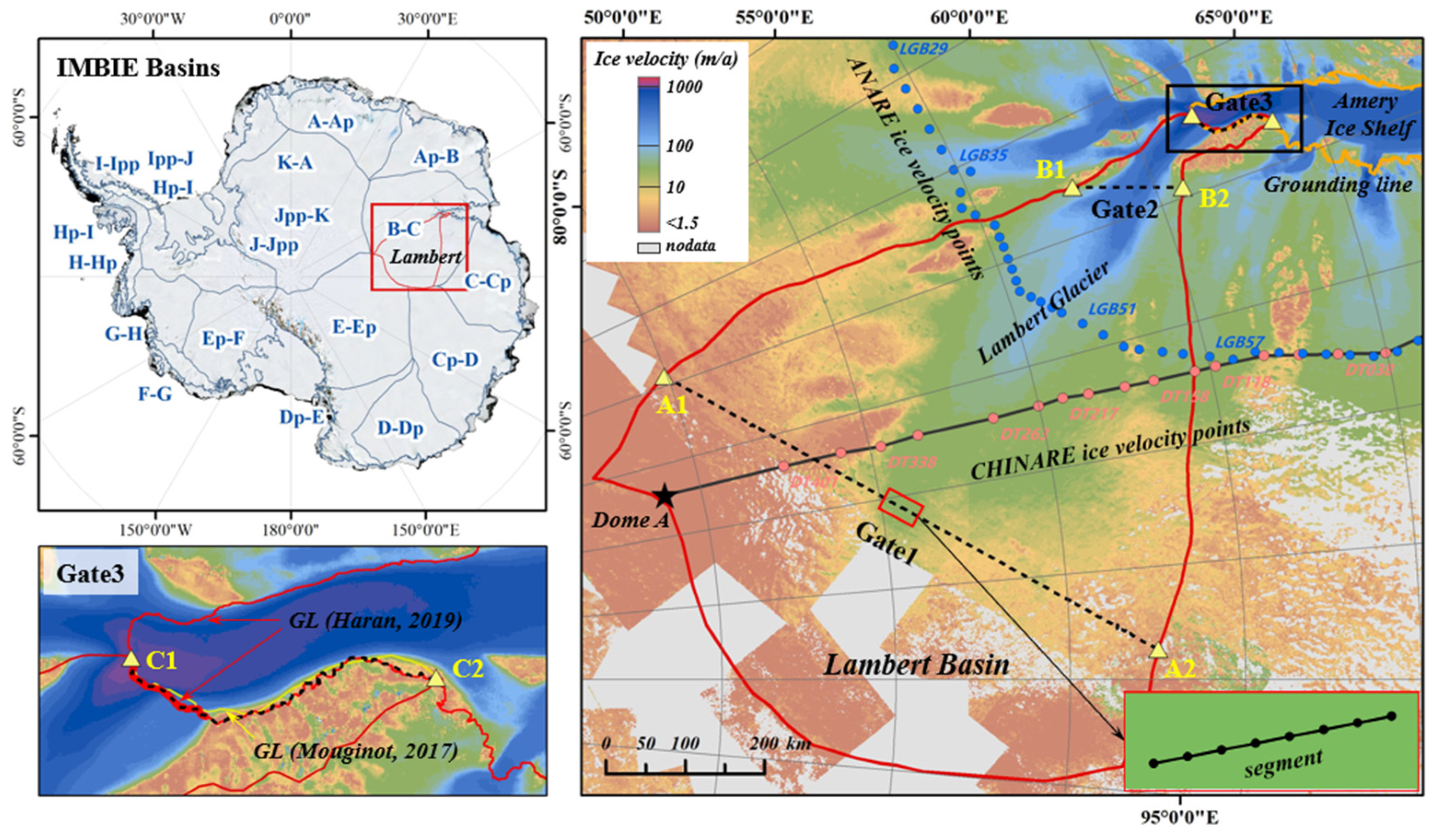
2.1.1. Drainage Basin Delineation and Grounding Line

The contour of the Antarctic glacier basin has been mapped by altimeter data, satellite hyperspectral imagery, and differential satellite interferometry synthetic aperture radar (DInSAR) data [32]. In this paper, the boundary of the Lambert Glacier in Antarctica was determined using version 2 of the Antarctic Basin Map compiled during the International Polar Year 2007–2009 (IPY) [25,26]. The data were obtained from the velocity data of interferometric SAR (InSAR) [33,34] combined with Bedmap2 data [20], updated in February 2018.
Since the change at the grounding line is relatively fast, the Moa2014_grounding_line_v01 with 125 m resolution obtained by NASA using satellite remote sensing images of Antarctic summer from 2013 to 2014 was selected as the grounding line [23,24]. These data provided high-quality cloudless Antarctic ice cover image data, which were updated in January 2019.
In this study, the Lambert Glacier area was demarcated with boundary information provided by the above two data, and the polar projection coordinates were transformed into Polar Stereographic for the mapping of other geographic data.

2.1.2. Ice Velocity

The surface ice velocity data were obtained from the Antarctic surface ice flow collected by Landsat-8. Shen Qiang et al. obtained a new high-resolution (105 m × 105 m) ice velocity product, the improved Antarctic-Wide Ice Flow Maps from LandSat-8 imagery (SH19), using 80,000 Landsat-8 optical images of the Antarctic region in summer from 2013 to 2019 [27]. SH19 resulted in the noise reduction of non-local means (NLM) filter and improved the quality assessment (QA) of band filtering using two-step optimization on the previous generation product. SH19 covers most of the areas from the Antarctic coast to 82.7°S stored in 500 m × 500 m grid size [27,35]. These data provide the clearest image of ice velocity in the Antarctic ice sheet to date with a 105 m grid spacing and provide Antarctic ice velocity data for 2018–2019. The mean value of the azimuthal difference on the main streamline (fast region) of the Lambert Glacier in the study area was almost 0, and the standard deviation of speed error was less than 4   m · a 1 , which was in good agreement with the field observation [27].
The surface ice velocity is a result of glacier creep deformation and the sliding of glacier bottom, and the speed of the whole ice column changes with depth [34]. The ice movement near the grounding line is dominated by basal sliding, thus the depth-averaged velocity used to calculate the ice flux was approximately equal to the surface velocity [15]. Combined with the two points, this paper considers only the influence of the surface slope and bottom slope at Gate 1 and Gate 2 on the ice depth-averaged velocity. The data used to calculate the surface slopes was obtained from ice surface elevation data with 500m grid resolution in MEaSUREs BedMachine Antarctica v2. The surface elevation data was obtained from the Reference Elevation Model of Antarctica (REMA), updated in 2019. BedMachine 500 m grid resolution bed topography map data were used for the bottom slope. The bed topography data were obtained by subtracting ice thickness from ice surface elevation [28,29].

2.1.3. Ice Thickness

The ice thickness data used in this paper were taken from MEaSUREs BedMachine Antarctica v2. These data were mainly based on the airborne survey data from 19 different research institutions since 1967. The dataset of AIS was obtained by using the method of mass conservation, and the continuity of ice thickness at the grounding line was ensured by using the ice shelf thickness data and hydrostatic equilibrium model [28,29]. The data update was added to the ICECAP2 digital elevation model (DEM) of the CHINARE program, which collected aerogeophysical data of the southern summer from 2015 to 2019 in the Princess Elizabeth Land (PEL) [36]. This update resulted in greater accuracy of the ice thickness data of the Lambert Glacier area. The grid resolution of ice thickness data was 500 m × 500 m, which was the same as data grid of the ice velocity used in this paper, avoiding the error caused by different spatial resolutions of data.

2.1.4. Surface Mass Balance

The input data of the mass balance were derived from the SMB of the regional semi-empirical atmospheric climate model RACMO2.3 with a spatial resolution of 27 km ∗ 27 km [30]. These data were obtained from the upgraded model of RACMO2 and widely used in the SMB simulation of AIS [37]. The Lambert Glacier lacks large-scale measured surface accumulation data. There were only some scattered points and the measured snow staked along the CHINARE DT traverse in Lambert Glacier [38], which were insufficient to estimate the SMB of the whole glacier. Cui (2020a) et al. compared the SMB results of 1997–2009 obtained by RACMO2.3 with the actual observation of SMB on the DT traverse from 2005 to 2008 and found that the correlation between them was greater than 76% [6]. Therefore, this paper used RACMO2.3 from 1979 to 2016 to estimate the SMB in the Lambert Glacier area.

2.2. Method

2.2.1. Ice Flux Calculation

Combined with the ice velocity, ice thickness, and ice gate location, the two adjacent grid points on each ice gate line were set as a segment (as shown in Figure 1). The starting points of calculation were A1, B1, and C1, respectively. The sum of ice flux on all segments was the total ice flux. The calculation is shown in Formula (1) [39]:
Q = i = 1 N ρ i H i l i U ¯ i  
where N is the total number of segments and i is the segment number, ρ i , H i , l i , and U i ¯   are the components of ice density, ice thickness, segment width, and depth-averaged velocity perpendicular to the ice gate in segment i, respectively.
The slope factor needed to be considered for calculating the ice velocity inside the glacier. To avoid the influence of micro-topography, we used Kriging interpolation method to downsample the above two kinds of DEM to 30 km × 30 km using GIS platform and estimated the slope by quadratic surface fitting [6]. The depth-averaged velocities U ( z ) ¯ at Gate 1 and Gate 2 positions were calculated as follows:
U ( z ) ¯ = U s 2 A n + 1 · τ b n · H + 2 A n + 2 · τ b n · H  
where A is the creep coefficient, n is the flow law exponent, τ b = f τ d , τ d is the shear stress, f denotes a scale factor (usually of order one), and H is the ice thickness. In this paper, A = 9 × 10 25   s 1   Pa 3 , and n = 3 [6,34,39]. Then, according to the angle between the vector direction of U ( z ) ¯ and the ice gate, the component U i ¯ perpendicular to the ice gate was obtained. The U i ¯ is the sine component of U ( z ) ¯ relative to ice gate.
To further improve the accuracy of calculated ice flux, the formula of an empirical density-depth relation was used to estimate the density ρ i corresponding to different thicknesses of each ice gate segment:
ρ i = 0 H   [ ρ ( ρ ρ s ) e ( z / z ρ ) ] d z / H  
where H is the ice thickness corresponding to a single segment; ρ is the density of the ice ( 917   kg · m 3 ); ρ s is the density of the firn layer ( 400   kg · m 3 ) [40]; z is the depth; z ρ is a constant value, which corresponds to a characteristic depth of the firn [39,41].
The error source of ice flux came mainly from the uncertainty of ice velocity and ice thickness. The error of velocity was obtained from the error diagram provided by Shen Qiang et al. [27], and the error range was 0 11.2   m · a 1 . The ice thickness error was taken from the error map of BedMachine Antarctica v2 [28,29]. As the ice thickness error in some regions was too large, the standard deviation of ice thickness error calculated by error conduction was controlled within 200 m. The error formula is:
δ q = i = 1 N Q i ( | δ v V i | + | δ h H i | )  
where δ q is the total error of ice flux, Q i is the ice flux of each segment, and δ v and δ h are the error values of ice velocity and thickness of each segment [31].

2.2.2. Ice Gate Location

Setting ice gates in the flow direction can simplify the mass balance calculation [15]. Based on the ice velocity and ice thickness data, the ice gates were set on the streamline with clear ice velocity variations and small ice thickness errors in Lambert Glacier. To control the error of ice flux to a small range, the standard deviation of ice thickness error on the ice gates was controlled at a maximum of no more than 200 m according to the error conduction. The locations of the ice gate are shown in Figure 1, and the latitude and longitude of the corresponding starting points and the length of the ice gate in polar coordinates are shown in Table 2. Under the two preconditions and calculation methods, the specific operation of determining positions of ice gates was as follows.
Gate 1 position: To estimate the contribution of ice movement in the upper reaches of the Lambert Glacier to the downstream ice flux, Gate 1 was determined in the southern region of the glacier. As shown in Figure 1, the ice velocity data were partially missing in this region, thus Gate 1 started from the downstream of the missing rectangular region. Lines with missing rates of ice velocity greater than 5% and standard deviation of ice thickness error greater than 100 m will be excluded. At the same time, the middle line of the three lines whose total ice flux difference between adjacent lines was ~5% is selected. Finally, the position of the ice gate was determined between points A1 and A2, a total of 1247 sections.
Gate 2 position: We determined the Gate 2 in the middle of ANARE LGB traverse and grounding line, and researched the gap between the ice flux through the middle of the convergence area and the ice flux through the grounding line. Since the uncertainty of ice thickness in this region was high, the measured lines with the standard deviation of ice thickness error greater than 200 m were firstly excluded, and then the method of determining G1 was used to calculate from the narrowest location to the upstream. Finally, the position of Gate 2 was determined to be between point B1 and B2, with a total of 280 segments.
Gate 3 position: Many studies have been conducted on the change in ice flux across the grounding line, but ice flux at the grounding line changes fast. We re-estimated the ice flux at the grounding line using the recently updated grounding line position. The different locations of the grounding line are shown in the lower left of Figure 1. The grounding line of the Lambert Glacier provided by MOA 2014 dataset was taken as the starting position, and the upstream adjacent ice gates were taken for calculation. The selection method was the same as before. Finally, Gate 3 was determined as the position of 500 m upstream of the starting position, and the ice flow through the ice gate to Amery ice shelf over the whole Gate 3 line was counted. A total of 212 segments were taken on Gate 3, of which the first 72 segments from the C1 position were obtained from the mainstream area, and the length of the mainstream area was similar to the length of the ice gate set by predecessors.

2.2.3. Surface Mass Balance Processing

The annual SMB data of RACMO2.3 from 1979 to 2016 were used to estimate the input mass of the Lambert Glacier [30]. First, we took the arithmetic average of the 38-year period from 1979 to 2016 at each point of the original RACMO2.3 data. Second, the Kriging interpolation method was used to resample the data into a grid size of 2 km × 2 km, and then the data of the area were cut out by using the geographic location mapping of the Lambert Glacier basin. The interpolated RACMO2.3 data points along the DT traverse in the Lambert Glacier and the in situ SMB data points compiled by Wang (2021) et al. [38] are shown in Figure 2. The mean value of the interpolated RACMO2.3 data on the Lambert Glacier was 53.98   kg / m 2 a 1 , while the mean value of the in situ SMB data compiled by Wang et al. along the DT traverse was 55.67   kg / m 2 a 1 .
According to the locations of the ice gates determined above, the total SMB of the upstream region of G1, the region between G1 and G2, the region between G2 and G3, and the whole glacier in Lambert Glacier were calculated, respectively. The total SMB was equal to the corresponding annual average accumulation rate multiplied by the region’s area, and the error was 20% of the SMB [42,43]. Finally, the subtraction with the output ice flux was used to estimate the net accumulation of the corresponding area within the Lambert Glacier.

3. Results and Discussion

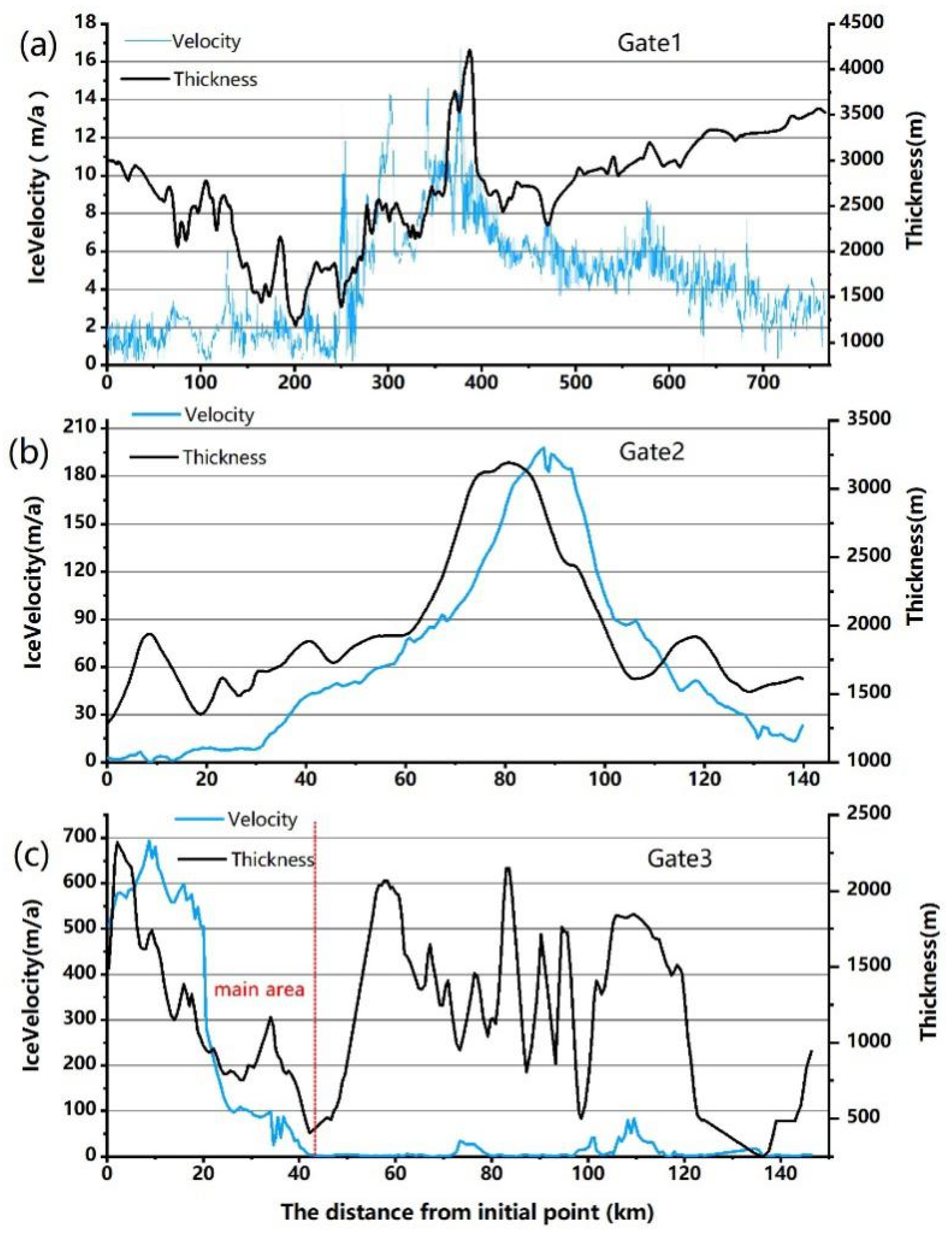
3.1. Depth-Averaged Velocity

Based on the method mentioned above, the changes of U i ¯ and H i corresponding to each segment of G1, G2, and G3 are shown in Figure 3 and Figure 4.
Figure 3a shows the G1 line. From the starting point, the component of about 250 km perpendicular to the ice gate was small, and the value of more than 87% U i ¯ was less than 3   m · a 1 . There was an increase of about 250–380 km along G1, and the speed peak was near the maximum of ice thickness. After reaching the peak, the U i ¯ of the remaining part of the G1 survey line tended to ease again, and the mean value of U i ¯ in the part of 640–780 km was less than 3.4   m · a 1 . The average ice velocity error in the part with large velocity (about 250–420 km) on the G1 was 0.6   m · a 1 , and the standard deviation of velocity error in the whole line was 0.5   m · a 1 . The standard deviation of the thickness error was 79 m, of which 74% was less than 50 m. In determining the Gate 1 location, the area located about 10 km upstream of Gate 1 did not meet the selection requirements set in this article. Additionally, in the latter half of the length of about 290 km (as shown in Figure 4), the ice thickness error was large (part of the ice thickness uncertainties are more than 500 m).
Figure 3b shows the G2 line, where the moving speed of the glacier was significantly greater than that of G1. As shown in Figure 3 and Figure 4, the glacier moved faster (>150   m · a 1 ) in the range of 40–95 km from point B1, and the direction of ice flow in this region showed that the ice movement had a clear trend of convergence to the middle. The changing trend of the U i ¯ value was roughly the same as that of ice thickness. The average velocity error on G2 was 5.7   m · a 1 , and the standard deviation was 1.1   m · a 1 . The thickness error of less than 50 m accounted for 43%, and the standard deviation of the error was 155 m. In the calculation process of determining the position of Gate 2, the area located about 13 km downstream of Gate 2 was not in line with the selection parameters set in this paper. As shown in Figure 4, the error of ice thickness in the region of about 10 km width was large (part of ice thickness uncertainties exceed 800 m).
Figure 3c shows the G3 line, and the change of ice velocity was different from that of G1 and G2. Located about 44 km from C3 was the mainstream area of G3, where the maximum component perpendicular to the ice gate reached 693.7   m · a 1 . On the G3 line, except for the mainstream, only a few areas of ice flow entered the Amery ice shelf through the grounding line. Unlike previous studies that only calculated the mainstream region [2,10,15], we also counted the output of the latter half of the grounding line (about 90–140 km along the line), and the corresponding ice movement was reflected in the ice flux calculation. The mean error of ice velocity on G3 was 6.7   m · a 1 , and the standard deviation was 3.88   m · a 1 . The percentage of segments with ice thickness error less than 50 m was 80%, and the standard deviation was 19 m.

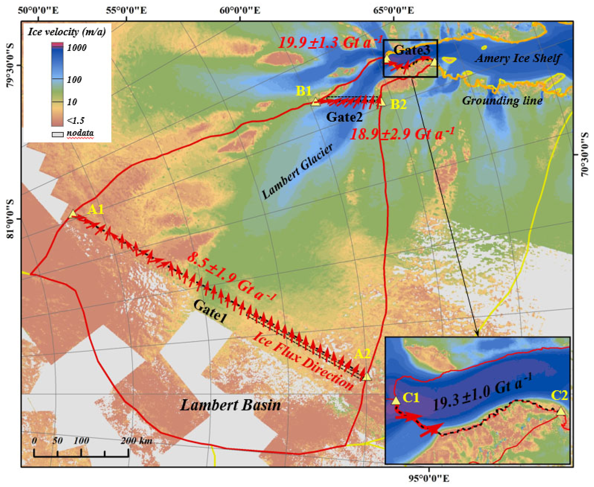
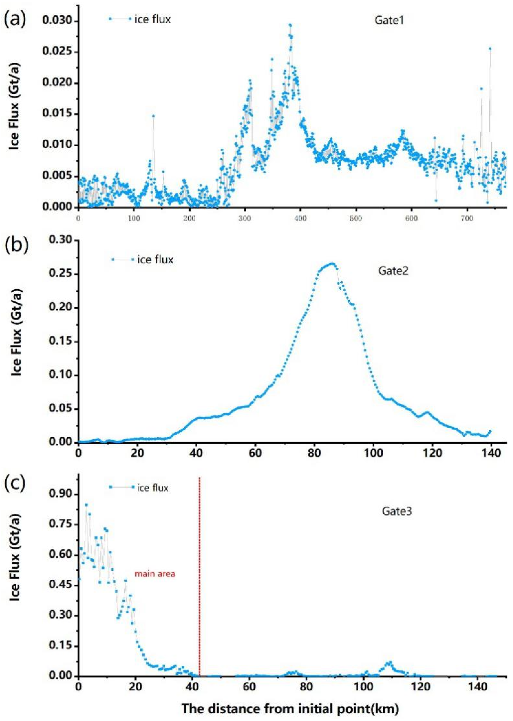
3.2. Ice Flux and Mass Balance

As shown in Figure 4, the ice flux through G1, G2, and G3 in the Lambert Basin during 2018–2019 was 8.5 ± 1.9   Gt · a 1 , 18.9 ± 2.9   Gt · a 1 , and 19.9 ± 1.3   Gt · a 1 , respectively. The ice flux from the mainstream region of G3 was 19.3 ± 1.0   Gt · a 1 . Details of the changes in ice flux on the ice gates are shown in Figure 5.
The main sources of ice flux error were evaluated according to the error of thickness and velocity. The dominant factor of ice flux error on G1 was the error of ice velocity, accounting for 83% of total error. As the ice velocity at both endpoints of G1 was very small, a minor change in velocity had a great statistically significant effect on the ice flux. In contrast, the effect of ice thickness errors on G1 was not significant. The ice flux error at G2 was mainly from the ice thickness error, accounting for 76% of flux error, mainly due to the sparse airborne survey lines in this area, resulting in low accuracy of ice thickness data and large fluctuation of error values. In the mainstream region of G3, the error of ice flux from ice thickness was 54%, and the error of total ice flux from ice thickness was 51%. The airborne geophysical observation was intensive, and the accuracy of ice thickness and ice velocity was greatly improved compared with G1 and G2.
Taking G1, G2, and G3 lines as the boundary, the SMB in the inner area of Lambert Glacier was estimated using RACMO2.3 model data. According to the ‘input–output’ reduction method (‘input flux’ + ‘accumulation’ − ‘output flux’), the mass balance in the region was obtained as follows: the mass balance of the Lambert Glacier was negative in the south of G1, the part between G1 and G2 was positive, and the part between G2 and G3 was negative. The whole Lambert Glacier was in a positive equilibrium with a net accumulation of 2.4 ± 3.5   Gt · a 1 , as shown in Table 3. Moreover, the ice flux and mass balance in the Lambert region were compared with previous studies. The change of ice flux flowing into the Amery ice shelf through the grounding line is shown in Table 4.
Studies on ice flux variations in inland areas of the upper Amery ice shelf were mostly conducted near ANARE LGB traverse [2,6,16]. H.L. Fricker et al. (2000) divided the LGB traverse route into three parts: the ‘West’ (LGB00-32), the ‘Streams’ (LGB32-56), and the ‘East’ (LGB56-72). The ‘Streams’ contain the mainstream of the Mellor glacier and the Lambert Glacier. The ice flux output from the ‘Streams’ was 21.8   Gt · a 1 [16]. Wen et al. (2007) calculated the ice flux of the LGB traverse route in the Lambert Glacier section (about LGB39–LGB55) as 17.4 ± 0.9   Gt · a 1 [2]. In this paper, the ice flux of 18.9 ± 2.9   Gt · a 1 (G2) was measured at approximately 170km downstream of the route. Cui et al. (2020) calculated the ice flux on the CHINARE DT traverse, of which the ice flux through the Dome A-LGB66 section was 20.9 ± 1.9   Gt · a 1 [6]. These results show that the Lambert Glacier has a significant contribution to the Lambert–Amery drainage system. Our studies also suggest that the gradual change of ice movement from inland to downstream (north of the G2) is verified by the ice flux on the G1. Compared with Cui et al., they only calculated the ice flux along the DT traverse. They did not calculate the ice flux that the glacier evidently flowed into the Amery ice shelf during the period, and the mass balance in the region was also estimated upstream of the DT traverse [6]. Our work in the Lambert Glacier took these gaps into account. At the same time, the latest remote sensing datasets were used to reflect the recent changes in the Lambert Glacier, especially in the use of ice velocity and BedMachine v2.
As shown in Table 4, Wen et al. (2007) found that the ice flux across the Lambert Glacier grounding line differs greatly from the results of the other three studies, mainly due to differences in ice thickness data. Wen et al. (2007) et al. used hydrostatics to calculate the ice thickness at the grounding line [2]. Yu et al. (2010) et al. used the ice thickness of the Bedmap (2001) [15]. Wen et al. (2014) used the Bedmap2 (2013) to update the ice thickness, while the ice thickness used in this paper was sourced from the BedMachine v2 (update 2021) [10]. The hydrostatic equilibrium model is susceptible to tides, which may lead to a large error in ice thickness and further cause excessive ice flux through the grounding line.
The results of Wen et al. (2014) and this study on the ice flux across the grounding line of the Lambert Glacier differ greatly, which may be due to reasons in the following explanation. Firstly, the update of ice thickness dataset: 1. Although both Bedmap2 dataset and BedMachine v2 dataset are based on airborne radar data, the grid resolution of Bedmap2 is 1 km, and that of BedMachine v2 is 500 m [20,28]; 2. BedMachine v2 uses hydrostatic equilibrium model and a firn densification model to further ensure the continuity of ice thickness at the grounding line, making the dataset more reliable [28,29]; 3. The BedMachine v2 data update included recently measured data, such as the results of the ICECAP2 DEM project, and more refined details of Antarctic bed topography [28]. Secondly, the change of grounding line location as shown in Figure 1, the grounding line position (red line) obtained from 2013 to 2014 at Gate 3 position moves southward compared with the grounding line position (yellow line) obtained from 2007 to 2009 [23,24,25,26]. Thirdly, the ice velocity in this paper uses the 2018–2019 data based on the LandSat-8 satellite. In recent years, global warming may cause the ice to move faster at the grounding line [27]. In addition, the grid resolution of the ice velocity is 500 m, which avoids redundant interpolation operations when matching with ice thickness. Finally, we estimate the density corresponding to different ice thicknesses according to Equation (2) instead of using the fixed ice density of 914   kg · m 3 (Wen et al., 2014) [10].
The calculated ice flux of Lambert Glacier passing through the mainstream area of grounding line was similar to results obtained by Yu (2010), but the positive accumulation within the Lambert Glacier was reduced from 3.6 ± 3.6   Gt · a 1 [15] to 2.4 ± 3.5   Gt · a 1 , and the floating range of ice flux error was also reduced.
In estimating the mass balance of the Lambert Glacier, excluding the negative results calculated by Wen (2007), the other three studies show that the region is in a state of positive equilibrium [2,10,15]. The detailed study on the interior of Lambert Glacier shows that positive accumulation of Lambert Glacier occurs in the central region (+4.1 ± 3.5   Gt · a 1 ), while negative accumulation occurs close to Dome A due to the low SMB rate and being within the vicinity of the grounding line due to the fast moving ice. It can be seen that although the Lambert Glacier is still in a positive accumulated state as a whole, the positive value of the glacier is reduced, indicating a possibility of mass loss in the region in the future. To some extent, the findings support the IMBIE team and Rignot et al. conclusions that the Antarctic is currently stable. At the same time, the uncertainty in the mass balance of the Lambert Glacier in EAIS is refined [1,21].

4. Conclusions

In this paper, the ice flux of the Lambert Glacier using recent updated methods was used to calculate ice velocity (2018–2019), grounding line (2013–2014, update 2019), glacier basin delineation (2007–2009, update 2018), and ice thickness (update 2021). According to the dataset of ice thickness and ice velocity, the ice gates, G1, G2, and G3 were selected at the upstream of Lambert Glacier, the glacier convergence, and the grounding line. The results show that the contribution of the ice flux in the Lambert Glacier from its upstream to the downstream during 2018–2019 was 8.5 ± 1.9   Gt · a 1 .The ice flux approximately 120 km from the grounding line in the downstream convergence region was 18.9 ± 2.9   Gt · a 1 . The total ice flux entering the Amery ice shelf through the grounding line was 19.9 ± 1.3   Gt · a 1 , and the ice flux from the mainstream (front around 44 km) was 19.3 ± 1.0   Gt · a 1 , which implies a dominant component. Compared with the large-scale Antarctic mass balance research completed by the IMBIE team and Rignot et al., this work performed a detailed analysis of the mass balance of the Lambert Glacier in East Antarctica and estimated the corresponding error [1,21]. Taking the ice gates G1, G2, and G3 as the boundaries, using the SMB of RACMO2.3, it was concluded that the SMB in the south of G1 in Lambert Glacier was 7.3 ± 1.5   Gt · a 1 , the regional SMB between G1 and G2 was 14.5 ± 2.9   Gt · a 1 , the partial SMB between G2 and G3 was 0.4 ± 0.0   Gt · a 1 ; there was a significant indigenous positive accumulation in the middle of Lambert (about 74–78°S, 67–85°E), and the value was 4.1 ± 3.5   Gt · a 1 . There was a negative accumulation in the south of G1 and the area between G2 and G3, and the values were 1.2 ± 2.4   Gt · a 1 and −0.6 ± 3.2   Gt · a 1 , respectively. The net accumulation in the whole glacier was 2.4 ± 3.5   Gt · a 1 . Compared with early 2000, the net accumulation of Lambert Glacier was significantly reduced, indicating the possibility of a future negative balance in the region [10,15].
The ice thickness data were retrieved from all current airborne physical detection data by the Mass Conservation method, yet the error of ice thickness in some areas remained large due to sparse airborne geophysical observations. Therefore, to evaluate the ice thickness and subglacial topography in this area more accurately, more in situ measurements are needed to optimize the details of basal conditions in the future. In addition, in the absence of large-scale SMB of in situ measurements in the Lambert Glacier, we used the regional atmospheric climate model RACMO2.3 to estimate the SMB of the entire glacier; however, the simulated SMB cannot accurately reflect the surface accumulation in this area. Hence, it is necessary to strengthen the observation of the large-scale SMB in the Antarctic ice sheet in the future to better quantify the mass balance of the AIS.

Author Contributions

Conceptualization, X.T.; methodology, X.T. and D.X.; software, D.X. and L.W.; validation, X.T. and B.S.; formal analysis, D.X. and X.T.; resources, X.T., S.Y. and Y.Z.; data curation, D.X; writing—original draft preparation, D.X. and X.T; writing—review and editing, D.X., L.L., X.T. and S.Y.; supervision, X.T. and Y.Z. All authors have read and agreed to the published version of the manuscript.

Funding

This work was funded by the National Natural Science Foundation of China (41941006 and 41876230), and the National Key R&D Program of China (Project No. 2019YFC1509102).

Data Availability Statement

The datasets of glacier basin delineation, grounding-line, and bedmachine v02 used in this paper are available at NSIDC. (https://doi.org/10.5067/AXE4121732AD; https://doi.org/10.5067/RNF17BP824UM; https://doi.org/10.5067/E1QL9HFQ7A8M), (1 July 2021); The improved Antarctic-Wide Ice Flow Maps from Landsat 8 Imagery published by Shen Qiang et al. are available at https://doi.pangaea.de/10.1594/PANGAEA.908845, (15 March 2021); The dataset of RACMO2.3 is available at https://www.projects.science.uu.nl/iceclimate/publictions/data/2018/index, (1 August 2021); The compilation of SMB records published by Wang et al. is available at https://doi.org/10.11888/Glacio.tpdc.271148, (1 August 2021).

Acknowledgments

We thank the space agency (NASA) for providing free satellite observation data to the entire scientific community so that our work could be successfully completed. We thank the PANGAEA platform for providing the new Antarctic ice velocity map published by Shen Qiang et al. We also thank Jan Melchior van Wessem et al. for disclosing RACMO2.3 and Yetang Wang et al. for providing the first ice-sheet-scale compilation of SMB records.

Conflicts of Interest

The authors declare no conflict of interest.

References

  1. Rignot, E.; Mouginot, J.; Scheuchl, B. Four decades of Antarctic Ice Sheet mass balance from 1979–2017. Proc. Natl. Acad. Sci. USA 2019, 116, 1095–1103. [Google Scholar] [CrossRef] [Green Version]
  2. Wen, J.H.; Jezek, K.C.; Csatho, B.M. Mass budgets of the Lambert, Mellor and Fisher Glaciers and basal fluxes beneath their flowbands on Amery Ice Shelf. SCES 2007, 50, 1693–1706. [Google Scholar] [CrossRef] [Green Version]
  3. Kingslake, J.; Ely, J.C.; Das, I.; Bell, R.E. Widespread movement of meltwater onto and across Antarctic ice shelves. Nature 2017, 544, 349–352. [Google Scholar] [CrossRef] [Green Version]
  4. Rignot, E.; Velicogna, I.; Broeke, M.R.V.D.; Monaghan, A.; Lenaerts, J.T.M. Acceleration of the contribution of the Greenland and Antarctic ice sheets to sea level rise. Geophys. Res. Lett. 2011, 38, 5. [Google Scholar] [CrossRef] [Green Version]
  5. Wouters, B.; Martin-Espanol, A.; Helm, V.; Flament, T.; van Wessem, J.M.; Ligtenberg, S.R.M.; Van Den Broeke, M.R.; Bamber, J.L. Dynamic thinning of glaciers on the Southern Antarctic Peninsula. Science 2015, 348, 899–903. [Google Scholar] [CrossRef] [PubMed]
  6. Cui, X.; Du, W.; Xie, H.; Sun, B. The ice flux to the Lambert Glacier and Amery Ice Shelf along the Chinese inland traverse and implications for mass balance of the drainage basins, East Antarctica. Polar Res. 2020, 39. [Google Scholar] [CrossRef]
  7. Golledge, N.R.; Levy, R.H.; Mckay, R.M.; McKay, R.M.; Naish, T.R. East Antarctic ice sheet most vulnerable to Weddell Sea warming. Geophys. Res. Lett. 2017, 44, 2343–2351. [Google Scholar] [CrossRef]
  8. Gong, Y.; Cornford, S.L.; Payne, A.J. Modelling the response of the Lambert Glacier–Amery Ice Shelf system, East Antarc-tica, to uncertain climate forcing over the 21st and 22nd centuries. Cryosphere 2014, 8, 1057–1068. [Google Scholar] [CrossRef] [Green Version]
  9. Pittard, M.L.; Galton-Fenzi, B.K.; Watson, C.S.; Roberts, J.L. Future sea level change from Antarctica’s Lambert-Amery glacial system. Geophys. Res. Lett. 2017, 44, 7347–7355. [Google Scholar] [CrossRef] [Green Version]
  10. Wen, J.; Huang, L.; Wang, W.; Jacka, T.; Damm, V.; Liu, Y. Ice thickness over the southern limit of the Amery Ice Shelf, East Antarctica, and reas-sessment of the mass balance of the central portion of the Lambert Glacier-Amery Ice Shelf system. Ann. Glaciol. 2014, 55, 81–86. [Google Scholar] [CrossRef] [Green Version]
  11. Budd, W.F.; Corry, M.J.; Jacka, T.H. Results From The Amery Ice Shelf Project. Ann. Glaciol. 1982, 3, 36–41. [Google Scholar] [CrossRef] [Green Version]
  12. Allison, I. The Mass Budget of the Lambert Glacier Drainage Basin, Antarctica. J. Glaciol. 1979, 24, 511. [Google Scholar] [CrossRef] [Green Version]
  13. Budd, W. The dynamics of the Amery Ice Shelf. J. Glaciol. 1966, 6, 335–358. [Google Scholar] [CrossRef] [Green Version]
  14. Higham, M.; Craven, M.; Ruddell, A.; Allison, I. Snow-accumulation distribution in the interior of the Lambert Glacier basin, Antarctica. Ann. Glaciol. 1997, 25, 412–417. [Google Scholar] [CrossRef] [Green Version]
  15. Yu, J.; Liu, H.; Jezek, K.C.; Warner, R.C.; Wen, J. Analysis of velocity field, mass balance, and basal melt of the Lambert Glacier–Amery Ice Shelf system by incorporating Radarsat SAR interferometry and ICESat laser altimetry measurements. J. Geophys. Res. Solid Earth 2010, 115, B11. [Google Scholar] [CrossRef] [Green Version]
  16. Fricker, H.A.; Warner, R.C.; Allison, I. Mass balance of the Lambert Glacier—Amery Ice Shelf system, East Antarctica: A comparison of computed balance fluxes and measured fluxes. J. Glaciol. 2000, 46, 561–570. [Google Scholar] [CrossRef] [Green Version]
  17. Jezek, K.C. RADARSAT-1 Antarctic Mapping Project: Change-detection and surface velocity campaign. Ann. Glaciol. 2001, 34, 263–268. [Google Scholar] [CrossRef] [Green Version]
  18. King, M.; Nguyen, L.N.; Coleman, R.; Morgan, P. Strategies for High Precision Processing of GPS Measurements with Application to the Amery Ice Shelf, East Antarctica. GPS Solut. 2000, 4, 2–12. [Google Scholar] [CrossRef]
  19. Lythe, M.B.; Vaughan, D.G. BEDMAP: A new ice thickness and subglacial topographic model of Antarctica. J. Geophys. Res. Solid Earth 2001, 106, 11335–11351. [Google Scholar] [CrossRef] [Green Version]
  20. Fretwell, P.; Pritchard, H.D.; Vaughan, D.G.; Bamber, J.L.; Barrand, N.E.; Bell, R.; Bianchi, C.; Bingham, R.G.; Blankenship, D.D.; Casassa, G.; et al. Bedmap2: Improved ice bed, surface and thickness datasets for Antarcti-ca. Cryosphere 2013, 7, 375–393. [Google Scholar] [CrossRef] [Green Version]
  21. The IMBIE Team. Mass balance of the Antarctic ice sheet from 1992 to 2017. Nature 2018, 558, 219–222. [Google Scholar] [CrossRef] [PubMed] [Green Version]
  22. IPCC. Climate Change 2021: The Physical Science Basis. Contribution of Working Group I to the Sixth Assessment Report of the Intergovernmental Panel on Climate Change; Cambridge University Press: Cambridge, UK, 2021; Chapter 9; Available online: https://www.ipcc.ch/assessment-report/ar6/ (accessed on 1 September 2021).
  23. Haran, T.; Klinger, M.; Bohlander, J.; Fahnestock, M.; Painter, T.; Scambos, T. MEaSUREs MODIS Mosaic of Antarctica 2013–2014 (MOA2014) Image Map, Version 1; NSIDC: National Snow and Ice Data Center: Boulder, CO, USA, 2018. [Google Scholar] [CrossRef]
  24. Scambos, T.A.; Haran, T.M.; Fahnestock, M. MODIS-based Mosaic of Antarctica (MOA) data sets: Continent-wide surface morphology and snow grain size. Remote Sens. Environ. 2007, 111, 242–257. [Google Scholar] [CrossRef]
  25. Mouginot, J.; Scheuchl, B.; Rignot, E. MEaSUREs Antarctic Boundaries for IPY 2007–2009 from Satellite Radar, Version 2; NSIDC: National Snow and Ice Data Center: Boulder, CO, USA, 2017. [Google Scholar] [CrossRef]
  26. Rignot, E.; Jacobs, S.; Mouginot, J.; Scheuchl, B. Ice-shelf melting around Antarctica. Science 2013, 341, 266–270. [Google Scholar] [CrossRef] [PubMed] [Green Version]
  27. Shen, Q.; Wang, H.; Shum, C.K.; Jiang, L.; Hsu, H.; Gao, F.; Zhao, Y. Antarctic-wide annual ice flow maps from Landsat 8 imagery between 2013 and 2019. Int. J. Digit. Earth 2020, 14, 597–618. [Google Scholar] [CrossRef]
  28. Morlighem, M. MEaSUREs BedMachine Antarctica, Version 2; NSIDC: National Snow and Ice Data Center: Boulder, CO, USA, 2020. [Google Scholar] [CrossRef]
  29. Morlighem, M.; Rignot, E.; Binder, T.; Blankenship, D.; Drews, R.; Eagles, G.; Eisen, O.; Ferraccioli, F.; Forsberg, R.; Fretwell, P.; et al. Deep glacial troughs and stabilizing ridges unveiled beneath the margins of the Antarctic ice sheet. Nat. Geosci. 2020, 13, 132–137. [Google Scholar] [CrossRef]
  30. Van Wessem, J.M.; van de Berg, W.J.; Noël, B.P.Y.; van Meijgaard, E.; Amory, C.; Birnbaum, G.; Jakobs, C.L.; Krüger, K.; Lenaerts, J.T.M.; Lhermitte, S.; et al. Modelling the climate and surface mass balance of polar ice sheetsusing RACMO2, part 2: Antarctica (1979–2016). Cryosphere 2018, 12, 1–35. [Google Scholar] [CrossRef] [Green Version]
  31. Taylor, J. Introduction to Error Analysis, the Study of Uncertainties in Physical Measurements, 2nd ed.; University Science Books: South Orange, NJ, USA, 1997; pp. 13–79. [Google Scholar]
  32. Rignot, E.; Mouginot, J.; Scheuchl, B. Antarctic grounding line mapping from differential satellite radar interferometry. Geophys. Res. Lett. 2011, 38, 10. [Google Scholar] [CrossRef] [Green Version]
  33. Mouginot, J.; Scheuchl, B.; Rignot, E. Mapping of Ice Motion in Antarctica Using Synthetic-Aperture Radar Data. Remote Sens. 2012, 4, 2753–2767. [Google Scholar] [CrossRef] [Green Version]
  34. Rignot, E.; Mouginot, J.; Scheuchl, B. Ice Flow of the Antarctic Ice Sheet. Science 2011, 333, 1427–1430. [Google Scholar] [CrossRef] [Green Version]
  35. Shen, Q.; Wang, H.; Shum, C.K.; Jiang, L.; Hsu, H.T.; Dong, J.; Mao, S.; Gao, F. Present-day high-resolution ice velocity map of the Antarctic ice sheet. Earth Syst. Sci. 2018, 1–25. [Google Scholar] [CrossRef] [Green Version]
  36. Cui, X.; Jeofry, H.; Greenbaum, J.S.; Guo, J.; Li, L.; Lindzey, L.E.; Habbal, F.A.; Wei, W.; Young, D.A.; Ross, N.; et al. Bed topography of Princess Elizabeth Land in East Antarctica. Earth Syst. Sci. 2020, 12, 2765–2774. [Google Scholar] [CrossRef]
  37. Van Wessem, J.M.; Reijmer, C.H.; Morlighem, M.; Mouginot, J.; Rignot, E.; Medley, B.; Joughin, I.; Wouters, B.; Depoorter, M.A.; Bamber, J.L.; et al. Improved representation of East Antarctic surface mass balance in a re-gional atmospheric climate model. J. Glaciol. 2014, 60, 761–770. [Google Scholar] [CrossRef] [Green Version]
  38. Wang, Y.; Ding, M.; Reijmer, C.H.; Smeets, P.C.J.P.; Hou, S.; Xiao, C. The AntSMB dataset: A comprehensive compilation of surface mass balance field observations over the Antarctic Ice Sheet. Earth Syst. Sci. Data 2021, 13, 3057–3074. [Google Scholar] [CrossRef]
  39. Cuffey, K.M.; Paterson, W.S.B. The Physics of Glaciers, 4th ed.; Elsevier: Burlington, NJ, USA; Oxford, UK, 2010; pp. 285–398. [Google Scholar]
  40. Ren, J.A. Traverse Expedition to the Lambert Glacier Basin, Eastern Antarctica. J. Glaciol. Geocryol. 1995. Available online: http://en.cnki.com.cn/Article_en/CJFDTOTAL-BCDT504.004.htm (accessed on 1 June 2021).
  41. Guo, J.; Yang, W.; Dou, Y.; Tang, X.; Greenbaum, J.S.; Dou, R.; Pan, Y.; Zhang, Y.; Ding, M.; Jiang, S.; et al. Historical surface mass balance from a frequency-modulated continuous-wave (FMCW) radar survey from Zhongshan station to Dome A. J. Glaciol. 2020, 66, 965–977. [Google Scholar] [CrossRef]
  42. Gardner, A.S.; Moholdt, G.; Scambos, T.; Fahnstock, M.; Ligtenberg, S.; Broeke, M.V.D.; Nilsson, J. Increased West Antarctic and unchanged East Antarctic ice discharge over the last 7 years. Cryosphere 2018, 12, 521–547. [Google Scholar] [CrossRef] [Green Version]
  43. Thakur, P.K.; Swain, A.K.; Dhote, P.R.; Kumar, P.; Kaushik, S.; Gajbhiye, D.; Mahagaonkar, A.; Sharma, V.; Dharwadkar, A.; Aggarwal, S.; et al. Satellite and ground based estimates for ice surface velocities in the part of central Dronning Maud Land, East Antarctica: Implications for ice flux calculations. Polar Sci. 2021, 30, 100737. [Google Scholar] [CrossRef]
Figure 2. The SMB data on CHINARE DT traverse are shown above. The black point is the average value of the actual observed SMB data from DT158 to Dome A from 1999 to 2011 on CHINARE DT traverse [38]. The purple dots are annual SMB data from 1979 to 2016 extracted from RACMO2.3.
Remotesensing 14 00391 g002
Figure 3. (ac) correspond to Gate 1, Gate 2 and Gate 3, respectively. The blue line represents the depth-averaged velocity perpendicular to the ice gate, and the black line represents the ice thickness at the corresponding position. The red dotted line represents the dividing line of the mainstream area on Gate 3.
Remotesensing 14 00391 g003
Figure 4. Ice flux through Gates 1, 2, and 3. The red arrows on the ice gate lines indicate the direction of the ice flow and are spaced at 20 km intervals. Located at 1 km upstream of Gate 1 and 1.5 km downstream of Gate 2, the dashed black boxes with sizes of about 290 km × 9 km and 140 km × 10 km are areas with large ice thickness errors. The ice fluxes through Gate 1 and Gate 2 are 8.5 ± 1.9 Gt · a 1 and 18.9 ± 2.9   Gt · a 1 , respectively. The total ice flux through Gate 3 is 19.9 ± 1.3   Gt · a 1 , and the ice flux through the mainstream is 19.3 ± 1.0   Gt · a 1 ,indicated by the enlarged window.
Remotesensing 14 00391 g004
Figure 5. (ac) are the segmented ice fluxes of Gate 1, Gate 2, and Gate 3, respectively. The dotted red line is the dividing line of the mainstream area on Gate 3.
Remotesensing 14 00391 g005
Table 1. Sources and usage of major data used to calculate ice fluxes.
ProductsVersionLocation and
Accessed Date
Usage
MEaSUREs Antarctic Boundaries for IPY 2007–2009 from Satellite RadarBasins_Antarctica_v02https://doi.org/10.5067/AXE4121732AD (1 July 2021)Drainage Basin
Delineation
MEaSUREs MODIS Mosaic of Antarctica 2013–2014 (MOA2014) Image MapMoa2014_grounding_line_v01https://doi.org/10.5067/RNF17BP824UM (1 July 2021)Grounding line
Present-day high-resolution ice velocity and footprints maps of the Antarctic ice sheetShen Qiang, Wang HanSheng, et al. (2020)https://doi.pangaea.de/10.1594/PANGAEA.908845 (15 March 2021)Ice Surface
velocity
MEaSUREs BedMachine
Antarctica
Bedmachine v2: Ice surface elevation & Bed topography maphttps://doi.org/10.5067/E1QL9HFQ7A8M (1 July 2021)Slope
MEaSUREs BedMachine
Antarctica
Bedmachine v2: Ice thicknesshttps://doi.org/10.5067/E1QL9HFQ7A8M (1 July 2021)Thickness
RACMO2.3p2ANT27_1979-2016 (yearly)https://www.projects.science.uu.nl/iceclimate/publictions/data/2018/index (1 August 2021)Surface mass
balance (SMB)
Table 2. The starting point, ending point, and length of three ice gates.
FluxGate NameInitial PointEnd PointDistance along Gate (km)
Gate 1 (G1)A1 (80.0333°S, 69.3335°E)A2 (75.0013°S, 88.6496°E)791.7
Gate 2 (G2)B1 (74.8872°S, 67.9234°E)B2 (73.7075°S, 69.6156°E)139.8
Gate 3 (G3)C1 (73.3088° S, 67.0301° E)C2 (72.4824° S, 68.4121° E)146.4
Table 3. Mass balance of upstream, middle, downstream, and whole Lambert Glacier.
LocationInput Flux
( G t · a 1 )
Accumulation from RACMO2.3
( G t · a 1 )
Output Flux
( G t · a 1 )
Net Budget
( G t · a 1 )
Average   Accumulation   Rate   ( k g / m 2 a 1 )
The south of G1/ 7.3 ± 1.5 8.5 ± 1.9 1.2 ± 2.4 40.84
G1–G2 8.5 ± 1.9 14.5 ± 2.9 18.9 ± 2.9 + 4.1 ± 3.5 67.74
G2–G3 18.9 ± 2.9 0.4 ± 0.0 19.9 ± 1.3 0.6 ± 3.2 48.14
Total Lambert/ 22.3 ±   3.3 19.9 ± 1.3 + 2.4 ± 3.5 53.98
Table 4. Accumulation, the ice flux across grounding-line and mass budget on Lambert Glacier from different studies.
StudiesArea
( k m 2 )
Accumulation
( G t · a 1 )
Ice Flux
( G t · a 1 )
Mass Budget
( G t · a 1 )
Wen (2007)424,930 22.6 ± 2.3 25.4 ± 2.5 2.8 ± 3.4
Yu (2010) 400,715 22.7 ± 2.3 19.0 ± 2.8 3.6 ± 3.6
Wen (2014) 424,930 18.2 ± 1.3 14.0 ± 1.7 4.2 ± 2.3
This Study 413,671 22.3 ± 3.3 19.9 ± 1.3 2.4 ± 3.5
Publisher’s Note: MDPI stays neutral with regard to jurisdictional claims in published maps and institutional affiliations.

