Article

Weighted Group Sparsity-Constrained Tensor Factorization for Hyperspectral Unmixing

1
College of Artificial Intelligence, Yango University, Fuzhou 350015, China
2
College of Computer Science and Techology, Zhejiang University, Hangzhou 310007, China
3
School of Artificial Intelligence, Xidian University, Xi’an 710071, China
*
Author to whom correspondence should be addressed.
Remote Sens. 2022, 14(2), 383; https://doi.org/10.3390/rs14020383
Submission received: 28 November 2021 / Revised: 3 January 2022 / Accepted: 10 January 2022 / Published: 14 January 2022

Abstract

:
Recently, unmixing methods based on nonnegative tensor factorization have played an important role in the decomposition of hyperspectral mixed pixels. According to the spatial prior knowledge, there are many regularizations designed to improve the performance of unmixing algorithms, such as the total variation (TV) regularization. However, these methods mostly ignore the similar characteristics among different spectral bands. To solve this problem, this paper proposes a group sparse regularization that uses the weighted constraint of the L 2 , 1 norm, which can not only explore the similar characteristics of the hyperspectral image in the spectral dimension, but also keep the data smooth characteristics in the spatial dimension. In summary, a non-negative tensor factorization framework based on weighted group sparsity constraint is proposed for hyperspectral images. In addition, an effective alternating direction method of multipliers (ADMM) algorithm is used to solve the algorithm proposed in this paper. Compared with the existing popular methods, experiments conducted on three real datasets fully demonstrate the effectiveness and advancement of the proposed method.

1. Introduction

Hyperspectral remote sensing images have a wide range of applications in the field of earth observation because of the rich spectral information [1,2,3]. However, the increase in spectral resolution usually results in a decrease in spatial resolution due to the influence of spectral splitting [4]. As a result, hyperspectral images generally have low spatial resolution, which leads to the inclusion of multiple substances in the image pixels. Therefore, mixed pixels are widely present in the hyperspectral images (HSI). The purpose of hyperspectral unmixing is to extract all pure materials (called endmembers) in the HSI and the percentage of endmembers in each pixel (called abundances) [5].
To solve the above-mentioned unmixing problem, numerous models have been proposed, the most popular of which is the linear mixed model (LMM). Under the LMM, each of the mixed pixels is regarded as the linear expression form of the endmembers, and the expression coefficients of endmembers constitute the abundance matrix [6] of the image. Among them, nonnegative matrix factorization (NMF) has been favored by researchers for its clear physical meaning and simple optimization process. The purpose of NMF is to find a base matrix of the original data and the expression coefficients under this base matrix [7]. In unmixing task, the optimized base matrix is the endmember matrix while the expression coefficient matrix is the abundance matrix. However, the solution of the simple NMF model is a non-convex problem, which leads to unstable unmixing results [8]. Therefore, to improve the performance of unmixing, many improved NMF-based unmixing methods have been proposed, for instance, sparse-based and spatial-based.
According to the prior of the distribution of ground objects, the endmembers in the mixed pixels in HSI are much smaller than the endmember spectral library [9]. Therefore, the abundance matrix is reasonably sparse. As a result, the sparsity constraint of abundance matrix becomes one of the most popular constraints. The  L 0 regularization is the most ideal sparse regularizer [10]. Unfortunately, the NMF-based unmixing algorithm with L 0 sparsity constraint is an NP-hard problem [11]. As an improvement, the  L p norm is widely used in the unmixing frameworks based on NMF to improve the stability and effectiveness of the algorithm. Guo et al. [12] uses the L 1 regularization to relax the L 0 regularization while [13] uses the L 2 regularization to constrain the abundance matrix. L 1 / 2 has also been proven to make the abundance matrix get a good sparse result [14,15]. Some methods also use the L 2 , 1 regularization to simultaneously explore the sparse structure in the abundance map [16], which has been proven to have good performance in the unmixing algorithm.
Besides, the spatial distribution of ground objects has the characteristics of local similarity and global similarity [17,18]. That is, there is a certain spatial similarity structure in HSI. Therefore, spatial similarity constraints are also really popular technics to improve the effectiveness of NMF-based methods. Lu et al. [19] propose a manifold regularization, which learns the global similarity structure of data to constrain the abundance matrix and force the abundance vectors of similar pixels to be similar. Manifold constraints have also proved by [20,21] to be a really effective way to explore the spatial structures. In [22], it is considered that the abundance of a pixel is the consistence as the average value of its neighboring pixels to maintain the smooth characteristics of HSI. In addition to these, the total variation regularization [23] and its variation [24] are also applied to the NMF-based unmixing algorithms, which can effectively retain the smoothing relationship of the image in the abundance matrix. In [25], the clustering algorithm is used to explore the global similarity relationship of pixels in the HSI, and it is combined with the NMF framework to improve the performance of unmixing.
The NMF-based methods mentioned above have significantly improved the performance of unmixing. Unfortunately, this kind of algorithms has a great flaw. The NMF-based framework reshapes the original 3-D HSI into a 2-D matrix before unmixing. This method of image reshaping severely destroys the 3-D cube structure of HSI, and it is difficult to completely explore the missing spatial information even if spatial regularization constraints are subsequently used [26]. To slow down the loss of information and make better use of all the spatial and spectral information in HSI, many researchers have begun to use nonnegative tensor factorization (NTF) instead of NMF framework to carry out unmixing tasks. The NTF framework directly treats HSI as a 3-D tensor, and regards the image as a whole during the optimization process, which can completely transfer all the spatial relationships of the original image to the abundance tensor.
Zhang et al. [27] innovatively applies tensor factorization (TF) to unmixing for the first time, which obtains performance comparable to NMF framework. The canonical polyadic decomposition-based (CPD) method is used to extract endmember matrix in [28]. However, this kind of methods decomposes the image into a finite number of rank-1 tensors, the number of which is generally much larger than the actual number of endmembers. Another TF method, tucker factorization, is also applied to the unmixing task in [29]. Regrettably, tucker factorization often fails to correspond the unmixing result with the actual distribution of objects. To make the result of TF method has a clear physical meaning, Qian et al. [26] propose a matrix-vector-based NTF (MV-NTF) method, which decomposes the HSI into multiple component tensors, then each component tensor is expressed by the outer product of a matrix and a vector. This method greatly promotes the application of NTF framework in unmixing task. In addition, many researchers add some effective regularizations to improve the effectiveness of the MV-NTF method. For instance, a spatial low-rank tensor regularization is proposed by [30,31] to maintain the sparsity of the abundance tensor. Sun et al. [32] uses a local spatial similarity constraint to explore the local smooth features of the data. A regularization for exploring the low-rank spatial structure of data is also introduced in [33]. The purpose is to preserve the HSI properties completely in the abundance tensor to improve the performance of unmixing. In addition, TV regularization has also been added to the NTF framework, such as [23,34].
Although the above methods have good performance in hyperspectral unmixing, the NTF-based models still have room for improvement in combining spatial and spectral information. According to [24], the difference image obtained after the image is differentiated along the horizontal and vertical directions is also sparse, which not only has zero elements, but also has zero connected regions in space. Therefore, a weighted group sparsity-constrained tensor factorization (WSCTF) method is proposed in this paper. Specifically, the HSI is differentiated along the horizontal and vertical directions at the same time to obtain two three-dimensional difference images firstly, which can explore the sparse structure of the HSI. Subsequently, the difference images are folded along the mode-1 and mode-2 to obtain two sparse matrices. Then, the  L 2 , 1 norm is used to constrain the sparse structure of difference matrix, which can not only maintain the sparseness of the difference image, but also constrain the zero connected region. To enhance the sparsity, the proposed method WSCTF also provides a weight for the sparsity constraint in vertical and horizontal directions. In addition, the  L 2 , 1 regularization is used to constrain the sparsity of the abundance tensor. In summary, the contributions of this paper can be concluded as:
  • A sparse constrained regularization is proposed to explore the sparse structure of the HSI differential image in the horizontal and vertical directions. In addition, weight coefficients are used to enhance sparsity.
  • The L 2 , 1 norm is utilized to constrain the sparse regularizer, and the L 2 , 1 norm is embedded in the NTF framework to maintain the sparsity of the abundance tensor.
  • The proposed algorithm WSCTF uses the alternating direction method of multipliers to iteratively optimize. Experiments on three real data prove the effectiveness of our algorithm.
The paper is arranged as follows. Section 2 introduces the concepts related to tensor and the unmixing framework based on NTF. The proposed method WSCTF and its optimization are described in detail in Section 3. The synthetic and real experimental results are analyzed in Section 4. Section 5 is the conclusion of this paper.

2. Related Work

2.1. Notation

According to experiences, a matrix is a two-dimensional array, and a tensor is an extension of the matrix. In this paper, an italic letter is used to represent a scalar, e.g., y and I. A vector is expressed by a regular lowercase letter, e.g.,  y R I × 1 . A matrix is given using a bold captial letter, e.g.,  M R I 1 × I 2 , and a tensor is defined as a calligraphic letter, e.g.,  Y R I 1 × I 2 × × I N .
Tensor Mode: Each dimension of a tensor is called a mode. For instance, the tensor Y R I 1 × I 2 × I 3 has 3 modes. Mode-n Unfolding: It can reshape a tensor to a matrix form. For example, given the tensor Y R I × J × K , the mode-n unfolding of Y is represented as:
Y < 1 > ( j 1 ) K + k , i = y i j k , Y < 2 > ( k 1 ) I + i , j = y i j k , Y < 3 > ( i 1 ) J + j , k = y i j k .
in which Y < 1 > is the mode-1 unfolding of tensor Y . Y < 2 > and Y < 3 > are the mode-2 and mode-3 unfolding, respectively.
Frobenius Norm: The Frobenius Norm of tensor Y R I × J × K is given by:
| | Y | | F = i = 1 I j = 1 J k = 1 K | y i j k | 2 1 / 2 .
Mode-n Product: Given a tensor Y , it can be expressed as Y = A × n M , in which A × n denotes the mode-n unfolding of tensor A .

2.2. NTF Unmixing Method

According to [35], the linear spectral mixing model can be represented as a linear combination by the endmember matrix and abundance maps. Specifically, given hyperspectral data Y R I × J × K , then it can be written as:
Y = A × 3 M + N ,
where A R I × J × P is the abundance tensor. A × 3 denotes the mode-3 unfolding of tensor A . And  M R I × J and N R I × J × K are the endmember matrix and noise tensor existing in HSI, respectively. Besides, I, J and K are the dimensions of hyperspectral data, and P is the number of endmembers. As a result, the unmixing model based on tensor factorization can be given by
J ( A , M ) = 1 2 Y A × 3 M F 2 ,
in which | | · | | F denotes the Frobenius norm. Since hyperspectral unmixing is a practical image processing process, there must be non-negative constraint here. In addition, the sum of the abundance coefficients inside each pixel should be one. These two properties create two constraints in the function (4). Specifically, the objective function (4) can be updated as:
J ( A , M ) = 1 2 Y A × 3 M F 2 , s . t . A 0 , A × 1 1 P = 1 I × J ,
in which A × 1 is mode-1 unfolding of the abundance tensor A .
Unfortunately, the above function (5) is a non-convex problem, which needs to be optimized for both the abundance A and the endmember matrix M . To improve the performance of the algorithm, Ref. [36] adds the L 2 , 1 sparsity constraint to the NTF unmixing model. Therefore, it can be given as:
J ( A , M ) = 1 2 Y A × 3 M F 2 + λ S A 2 , 1 s . t . A 0 , A × 1 1 P = 1 I × J .
In addition, some spatial constraints are also added to the NTF unmixing model to explore the spatial information of HSI, especially TV regularization [34]. Specifically, the NTF unmixing model based on the TV regularization can be described as follows:
J ( A , M ) = 1 2 Y A × 3 M F 2 + λ S A 2 , 1 + λ T V A T V s . t . A 0 , A × 1 1 P = 1 I × J ,
where A T V is the TV regularization, and  λ T V denotes the weight parameter. Since the TV regularization has achieved excellent results in the spatial relationships of data, especially in maintaining the smoothness of the data, it has achieved comparable performance on the hyperspectral unmixing, which has been proved in [37,38]. However, the existing methods are still unable to fully explore some important characteristics of data. For instance, few work consider continuity in the direction of the spectral dimension. In addition, according to [39], the three-dimensional difference images obtained after also have group sparsity. Based on these ideas, this paper explores the three-dimensional spatial structure information of the image, including the spectral similarity of the difference images and the sparsity of the spatial group.

3. Proposed Method

In response to the questions mentioned above, a new regularization is designed to explore the spectral continuity and group sparsity of difference images of HSI. As a result, a weighted group sparsity constraint non-negative tensor factorization (WSCTF) method for hyperspectral unmixing is proposed. The proposed algorithm and its optimization method are described in detail in this section.

3.1. WSCTF Model

According to the existing experience, the TV regularization is widely used to explore the spatial smooth structure in HSI. Specifically, the TV regularizer can be expressed as follows:
A T V = D A 1 = D 1 A 1 + D 2 A 1 ,
where D denotes the difference operator. D 1 and D 2 are vertical and horizontal difference, respectively. | | · | | 1 is the l 1 norm. In detail, given the spatial coordinate of a abundance tensor ( i , j , p ) , then the difference results in the vertical and horizontal directions can be described as:
D 1 A i , j , p = A i , j + 1 , p A i , j , p , D 2 A i , j , p = A i + 1 , j , p A i , j , p .
Based on the above analysis, it can be concluded that the difference images in the horizontal and vertical directions are also three-dimensional tensors. According to the prior, the difference image has continuity in the spectral dimension. In addition, the difference image has extremely high sparsity. In the difference image, not only many elements are zeros, but also some connected regions with zeros elements. Therefore, a new weighted sparsity regularization is designed to explore these properties. Specifically, the regularization can be given as:
( A ) = | | W 1 ( D 1 A × 1 ) | | 2 , 1 + | | W 2 ( D 2 A × 2 ) | | 2 , 1 ,
in which W 1 and W 2 are aiming at enhancing the sparsity of difference images. A × 1 and A × 2 are the mode-1 and mode-2 unfolding of tensor A . | | · | | 2 , 1 denotes the l 2 , 1 norm, which can be used to explore the group sparsity of difference image. Therefore, the objective function (7) can be improved by:
J ( A , M ) = 1 2 Y A × 3 M F 2 + λ S A 2 , 1 + λ ( A ) s . t . A 0 , A × 1 1 P = 1 I × J ,
where λ is regularization parameter. In addition, to be more prepared to explore the sparse structure of the abundance tensor A , a weight constraint is also added to the sparse regularization. Finally, the objective function of WSCTF proposed in this paper can be expressed as:
J ( A , M ) = 1 2 Y A × 3 M F 2 + λ S W S A 2 , 1 + λ ( A ) s . t . A 0 , A × 1 1 P = 1 I × J ,
in which W s is the weight to promote the sparsity of abundance tensor. In the proposed method, not only the spatial neighborhood smoothing information is considered, but also the sparsity characteristics of the difference image, especially the group sparsity, are described. The optimization method of objective function (12) is explained in detail in the next subsection.

3.2. Optimization

The Formula (12) is a non-convex problem, which is directly difficult to solve. According to the exist experience, the ADMM algorithm is used to update each variable, which can be solved by decomposing the original problem into multiple sub-problems.
(1) Update M: For the function (12), it first considers the update of the endmember matrix M . At this time, the abundance tensor A is fixed, so the objective function can be expressed as:
J ( A , M ) = 1 2 Y A × 3 M F 2 .
It can directly obtain the updated rule of endmember M as:
M M . ( Y × 3 A × 3 T ) . / ( M A × 3 A × 3 T ) ,
in which Y × 3 and A × 3 are the mode-3 unfolding of tensors. . and . / are multiplication and division operators.
In addition, by introducing six intermediate variables G 1 , G 2 , G 3 , G 4 , G 5 and G 6 , the Formula (12) can be rewritten as:
min A , M 1 2 G 1 Y F 2 + λ s W S G 2 2 , 1 + λ W 1 G 3 2 , 1 + λ W 2 G 4 2 , 1 + l R + G 5 + l { 1 } G 6 , s . t . G 1 = A × 3 M , G 2 = A , G 3 = D 1 A × 1 , G 4 = D 2 A × 2 , G 5 = A , G 6 = A .
In the above Formula (15), G 5 and G 6 are used to meet the abundance nonnegative constraint (ANC) and abundance sum-to-one constraint (ASC). They are defined as:
l R + ( X ) = 0 , i f X 0 , + , o t h e r w i s e . l { 1 } ( X ) = 0 , i f sum ( X × 3 ) = 1 , + , o t h e r w i s e .
in which 1 denotes a matrix with all ones. Hence, the Lagrangian function of objective function (15) is:
min A , M , G i 1 2 G 1 Y F 2 + λ s W S G 2 2 , 1 + λ W 1 G 3 2 , 1 + λ W 2 G 4 2 , 1 + l R + G 5 + l { 1 } G 6 + μ 2 G 1 A × 3 M + H 1 F 2 + μ 2 G 2 A + H 2 F 2 + μ 2 G 3 D 1 A × 1 + H 3 F 2 + μ 2 G 4 D 2 A × 2 + H 4 F 2 + μ 2 G 5 A + H 5 F 2 + μ 2 G 6 A + H 6 F 2 .
(2) Update  A : In problem (17), the subproblem of A can become:
min A μ 2 G 1 A × 3 M + H 1 F 2 + μ 2 G 2 A + H 2 F 2 + μ 2 G 3 D 1 A × 1 + H 3 F 2 + μ 2 G 4 D 2 A × 2 + H 4 F 2 + μ 2 G 5 A + H 5 F 2 + μ 2 G 6 A + H 6 F 2 .
In problem (18), it can be directly solved by:
A × 3 M T M + k = 1 2 A × k ( D k T D k ) + 3 A = K
where
K = ( G 1 + H 1 ) × 3 M T + ( G 3 + H 3 ) × 1 D 1 T + ( G 4 + H 4 ) × 2 D 2 T + ( G 2 + H 2 + G 5 + H 5 + G 6 + H 6 )
(19) is equal as
A ( 3 ) T M T M + CA ( 3 ) T + 3 A ( 3 ) T = K ( 3 ) T
where C = [ I D 1 T D 1 ] + [ D 2 T D 2 I ] . C is a matrix with a locking loop structure. It can be easily concluded that M T M is a symmetric matrix. According to [39], 2-D fast Fourier transformation and SVD is employed to solve C and M T M , respectively. Then it can be obtained that C = F 2 T Ψ 2 F 2 and M T M = U 2 U 2 T , in which F 2 is a 2-D discrete Fourier transformation matrix. Then the update rule of A is
A = F o l d 3 ( [ F 2 T ( ( 1 T 2 ) ( F 2 K ( 3 ) T U 2 ) ) U 2 T ] T )
in which T 2 = ( d i a g ( Ψ 2 ) , d i a g ( Ψ 2 ) , , d i a g ( Ψ 2 ) ) + ( d i a g ( ) , d i a g ( ) , , d i a g ( ) ) T .
(3) Update the intermediate variables G i :
min G i 1 2 G 1 Y F 2 + l R + G 5 + l { 1 } G 6 + μ 2 G 1 A × 3 M + H 1 F 2 + μ 2 G 2 A + H 2 F 2 + μ 2 G 3 D 1 A × 1 + H 3 F 2 + μ 2 G 4 D 2 A × 2 + H 4 F 2 + μ 2 G 5 A + H 5 F 2 + μ 2 G 6 A + H 6 F 2 .
It can be easily concluded that the update formula of G 1
G 1 1 1 + μ Y + μ A × 3 M H 1 .
According to [40], the update rules related to G 2 can be expressed as:
G 2 = | | H 2 ( i , j , : ) | | 2 W S ( i , j ) λ s μ | | H 2 ( i , j , : ) | | 2 H 2 ( i , j , : ) , i f W S ( i , j ) λ s μ < | | H 2 ( i , j , : ) | | 2 , 0 , otherwise .
Observing the problem (19), it can be seen the intermediate variables G 2 , G 3 , and  G 4 have similar forms. Hence, their solving rules are also similar, then the closed solutions of G 3 and G 4 can be directly obtained as:
G 3 = | | C 1 ( i , j , : ) | | 2 W 1 ( i , j ) λ μ | | C 1 ( i , j , : ) | | 2 H 3 ( i , j , : ) , i f W 1 ( i , j ) λ μ < | | C 1 ( i , j , : ) | | 2 , 0 , otherwise .
where C 1 = D 1 A × 1 + H 3 .
G 4 = | | C 2 ( i , j , : ) | | 2 W 2 ( i , j ) λ μ | | C 2 ( i , j , : ) | | 2 H 4 ( i , j , : ) , i f W 2 ( i , j ) λ μ < | | C 2 ( i , j , : ) | | 2 , 0 , otherwise .
where C 2 = D 2 A × 2 + H 4 .
It is worth noting that both W s , W 1 and W 2 are weight matrixes, which are used to increase the degree of the sparsity. Therefore, their update rules can be described as:
W s ( i , j , k ) = 1 | G 2 ( i , j , k ) | + ε ,
W 1 ( i , j ) = 1 | | C 1 ( i , j , : ) | | 2 + ε ,
W 2 ( i , j ) = 1 | | C 2 ( i , j , : ) | | 2 + ε ,
in which ε is a small positive number.
Besides, G 5 and G 6 are aiming at ensuring ANC and ASC of abundance. Therefore, the update rule of them can be written as:
G 5 max A H 5 , 0 ,
G 6 A H 6 + repmat ( N , I ( 1 ) , 1 ) ) , N = 1 P 1 sum ( ( A H 6 ) ) .
(4) Update the Lagrange multipliers H i :
H 1 = H 1 A × 3 M + G 1 , H 2 = H 2 A + G 2 , H 3 = H 3 D 1 A × 1 + G 3 , H 4 = H 4 D 2 A × 2 + G 4 , H 5 = H 5 A + G 5 , H 6 = H 6 A + G 6 .
In general, the framework of the algorithm WSCTF proposed in this paper is summarized in Algorithm 1.
Algorithm 1 The proposed method SCLT
Input:
       Y R I × J × K —the mixing hyperspectral data; P—the number of endmembers;
      Parameter λ S , and  λ .
1.
Update the endmember matrix M by (14);
2.
Update the abundance tensor A via (22);
3.
Update the variables G 1 by (24), G 2 by (25), G 3 by (26), G 4 by (27), G 5 and G 6 via (31) and (32);
4.
Update the Lagrangian multipliers H 1 , H 2 , H 3 , H 4 , H 5 , H 6 by (33).
Output:
       A —the abundance tensor; M —the endmember matrix.

4. Experiments

To verify the effectiveness of the WSCTF algorithm proposed in this paper, this section conducts related experiments on two sythetic data and real data sets of Cuprite, Jasper Ridge and Samon, and discusses the experimental results in detail. Since the proposed WSCTF is based on a non-negative tensor decomposition algorithm, the five comparison algorithms used here are: ULTRA-V [30], SULRSR-TV [24], MV-NTF [26], NMF-QMV [41], NL-TSUn [33]. It is worth noting that ULTRA-V, MV-NTF and NL-TSUn are all based on NTF, while SULRSR-TV and NMF-QMV are based on NMF. In addition, the SULRSR-TV algorithm also uses the TV regularization to constrain the local smooth structure of the abundance. The purpose of setting up these comparative experiments is to comprehensively verify the effectiveness of our algorithm.
Spectral angle distance (SAD) and root-mean-square error (RMSE) are the most widely used evaluation indicators in unmixing tasks. Among them, SAD is used to describe the spectral angular distance between the estimated endmember and the ground truth. Correspondingly, the distance of the estimated abundance and the ground truth is described by RMSE. They can be expressed in mathematical formulas as:
RMSE = A A ^ 2 , SAD = cos 1 M ^ T M M ^ M
in which A ^ and M ^ are the ground truth of abundances and endmembers, respectively. Besides, to ensure the fairness of comparison, all experiments use the same experimental platform and use the vertex component analysis (VCA) and fully constrained least squares (FCLS) algorithm to initialize the endmembers and abundances. In addition, it is worth noting that the average and variance of the results of all experiments have been presented after 20 runs, which can illustrate the stability of algorithms.

4.1. Sythetic Data

Firstly, experiments are conducted on two synthetic data. All pure endmember spectra in the data are randomly sampled from the USGS spectral library [42].
(1) Dataset 1 (DS1): Set the number of endmembers p = 5 , the size of the HSI is 75 × 75 × 224 , where 224 is the number of spectral band. The specific data synthesis method is similar to the paper [34]. It is worth noting that each pixel here should comply with the LMM and meet the abundance ANC and ASC at the same time. Figure 1a shows the false color image of DS1.
(2) Dataset 2 (DS2): DS2 can form a control group with DS1. Here, the method described in [34] is used to synthesize DS2. Set the image size of DS2 to 90 × 90 × 224 , where 224 is the spectral band. Figure 1b shows the false color image of DS2. According to the above, two clean synthetic data can be obtained. Subsequently, 10 dB, 20 dB and 30 dB Gaussian noise are added to DS1 and DS2 respectively to form six data interfered by different noises. All experiments are all performed on these six data, which can prove the effectiveness of algorithms under different image sizes, different noise conditions, and different numbers of endmembers.
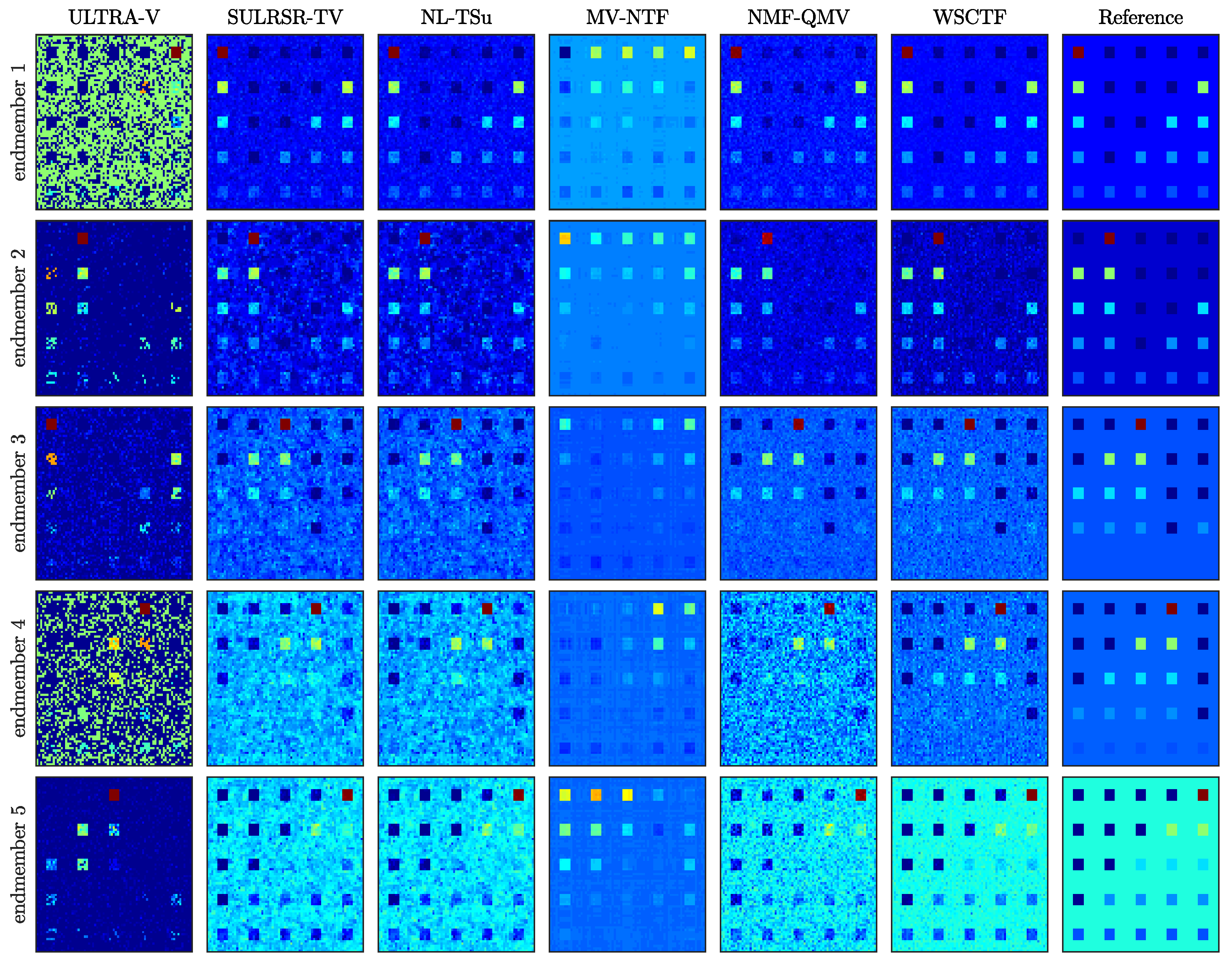
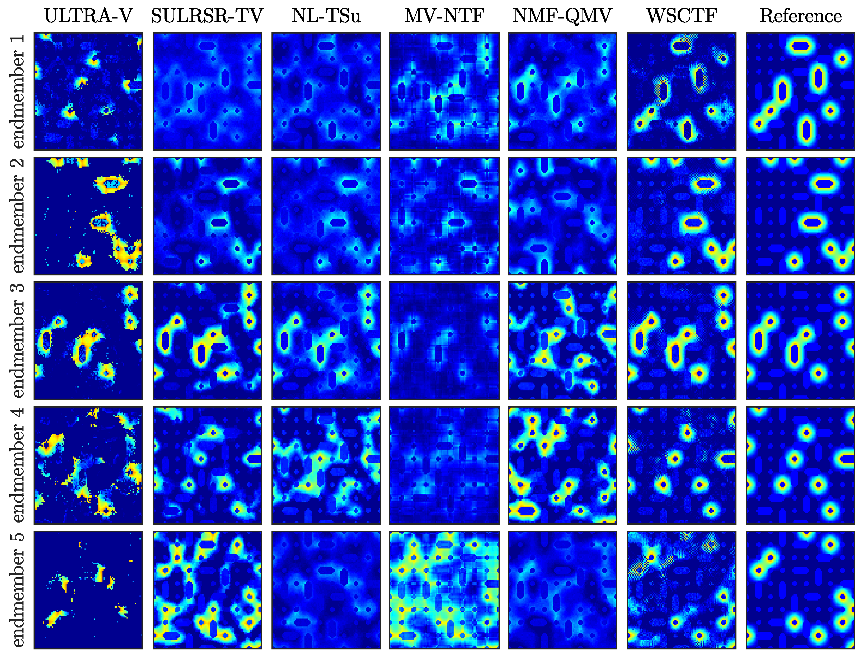
The SAD and RMSE results of the proposed WSCTF and five comparison algorithms on these six data are shown in Table 1 and Table 2. According to the results of Table 1 and Table 2, we can analyze the results: (1) On the DS1 and DS2 data, as the noise continues to increase, the performance of all algorithms, including the proposed WSCTF, is declining. However, the performance of WSCTF method changes less under the influence of different noises and the performance is more stable than other methods, since it fully considers the spatial and spectral similarity. (2) MV-NTF performs poorly on both data, because MV-NTF is based on the NTF basic algorithm, and other algorithms are mostly improved methods on it. (3) Since DS2 is more complicated than DS1 and the number of endmembers is more, all algorithms perform slightly worse on DS2. The ULTRA-V algorithm is mainly proposed for the variability with endmembers, but the absence of variable endmembers in the settings of DS1 and DS2 leads to poor unmixing performance. (4) The lack of pure pixels in the DS2 is the main reason for the low performance of the SULRSR-TV method. SULRSR-TV assumed that there must be pure pixels in the image when unmixing. In summary, compared with other comparison algorithms, the proposed WSCTF has certain advantages under the conditions of different noises, different image sizes and different numbers of endmembers. The above analysis can also be verified in the visualization results of abundance. As shown in Figure 2, the abundance and groundtruth obtained by all algorithms are displayed on DS1 with 20 dB. The abundance map estimated by the WSCTF method is obviously better than other comparison algorithms. Due to the large number of endmembers in DS2 with 20 dB, only five abundances are shown in Figure 3 here.

4.2. Real Datasets

Secondly, experiments are conducted on three real datasets.
(1) Jasper Ridge Data: Jasper Ridge data is a data set widely used to test the performance of unmixing algorithms, covering the Jasper Ridge Natural Reserve in California, USA. The data contains 224 spectral bands from 300 nm to 2500 nm, and its spectral resolution is 9.46 nm. Figure 1c is a pseudo-color image of Jasper Ridge data. Here we use an image with a size of 100 × 100 pixels to verify the performance of all algorithms. Because some bands are severely interfered by moisture and noise during the acquisition process, 188 bands are finally used for testing after removing these bands. According to a prior, there are four end members in this area, including soil, water, road and trees.
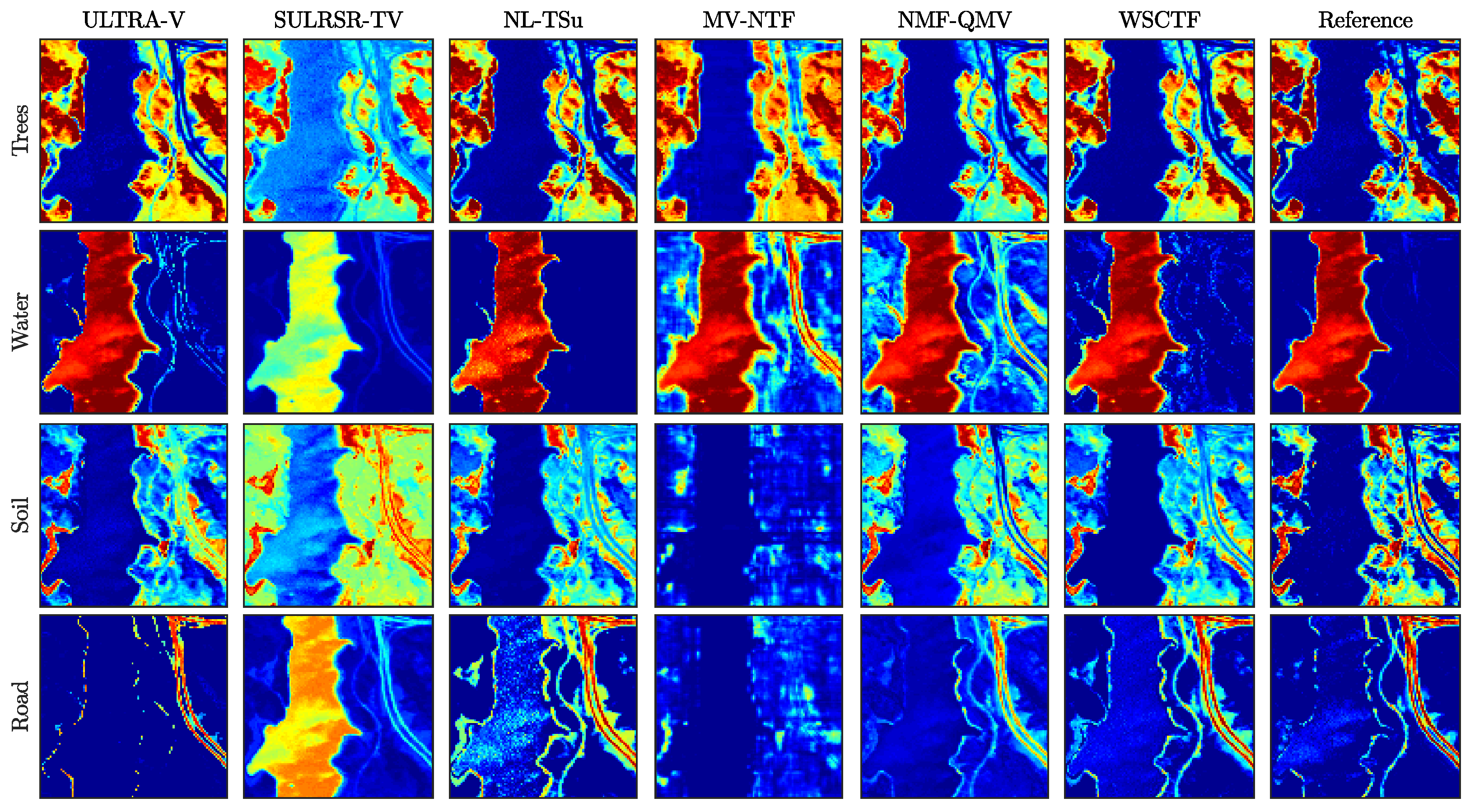
Table 3 shows the SAD results of the endmembers extracted by the proposed WSCTF compared with ground truth. The bold font indicates the best result. It can be concluded that the WSCTF method proposed in this paper has great advantages in the extraction of two endmembers, and the final SAD result is also optimal. In addition, the endmember spectra extracted by all algorithms are shown in Figure 4. Compared with the reference spectrum, it can be seen that the proposed algorithm has considerable advantages in endmember extraction compared with other methods. Figure 5 is the comparison result of all abundances, which can be concluded that the WSCTF algorithm is the closest to the reference. In addition, compared with the distribution of ground objects in the original image in Figure 1c, the accuracy of the proposed algorithm can also be inferred.
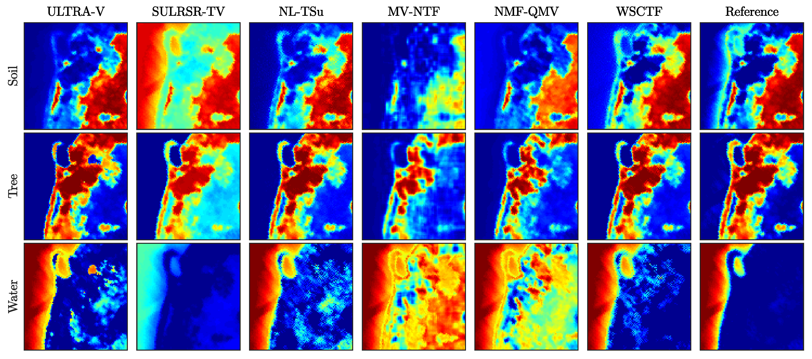
(2) Samon Data: According to [43], the samon data set is collected by the Florida Environment Research Institute through the Samon sensor. The data contains 156 bands and the spectral resolution is 3.13 nm. Here we are experimenting on an image with a size of 100 × 100 pixels. There are three types of ground features in this area, including water, soil and trees. Figure 1d is a pseudo-color image of Samon data. The SAD and its variance results extracted by the six methods on the Samon data are introduced in Table 4. Obviously, it can be concluded that all unmixing algorithms, including the WSCTF proposed in this paper, perform slightly worse on the endmember of water. Since the edge of water when it is mixed with the land is not easy to determine, the abundance map of the water body endmember is greatly disturbed. Similar conclusions can also be drawn from the visualization results in Figure 6 and Figure 7. However, it is gratifying that the method proposed in this paper has a great advantage in the separation of the endmember of water compared to other algorithms, which proves the superiority and stability of WSCTF proposed in this paper.
(3) Cuprite Data: This data set is also widely used in unmixing task. Its coverage area is a mining area, so there are many highly mixed pixels. Here, a subgraph with a size of 200 × 150 × 188 is intercepted to test the effectiveness of the algorithm, where 188 is the number of bands. Figure 1e is a pseudo-color image of Cuprite data. According to a prior, there are 12 pure mineral endmembers in this area. Unlike the Samon and Jasper Ridge data, the Cuprite data does not provide true values, so the ground truth of endmembers here are set using the method in [34].
Cuprite data mainly contains 12 minerals, namely Alunite, Kaolinite #1, Kaolinite #2, Sphene, Andradite, Nontronite, Muscovite, Pyrope, Chalcedony, Dumortierite, Montmorillonite, and Buddingtonite. Table 3 shows the SAD comparison results of the endmembers extracted by the six algorithms and the reference endmembers. As shown in Table 5, the algorithm proposed in this paper has obvious advantages in each endmember and average endmember results, and there are 7 optimal results. In addition, Figure 8 and Figure 9 are the visualized results of endmembers and abundance obtained after unmixing, respectively. In Figure 8, compared with the other five methods, it is obvious that the endmember spectrum obtained by the WSCTF algorithm is closer to the reference spectrum. The abundance maps are shown in Figure 9. Compared with [34], it can be seen that the proposed WSCTF can also obtain more accurate abundance results.

4.3. Parameter Analysis

The WSCTF algorithm proposed in this paper involves two sparse parameters λ and λ s . Here we take Jasper Ridge data as an example for parameter setting discussion. First, set λ as 0.015, and λ s to {0, 1 × 10 3 , 2 × 10 3 , 3 × 10 3 , 4 × 10 3 , 5 × 10 3 , 6 × 10 3 , 7 × 10 3 , 8 × 10 3 , 9 × 10 3 , 1 × 10 2 }. The setting of 0 can verify the advantages of the regularization proposed by this algorithm. It can be seen from Figure 10a that when λ s =0.015, WSCTF achieves the best results on Jasper Ridge data. Then set λ s as 0.015, λ to {0, 1 × 10 3 , 2 × 10 3 , 3 × 10 3 , 4 × 10 3 , 5 × 10 3 , 6 × 10 3 , 7 × 10 3 , 8 × 10 3 , 9 × 10 3 , 1 × 10 2 }. The result is shown in Figure 10b, and when λ = 0.02, WSCTF achieves the best results on Jasper Ridge data. Similarly, apply the same method to other data sets to ensure the optimal parameters. Finally, the results of the parameters set in this paper are shown in Table 6. It is worth noting that the same parameters are set here for DS1 and DS2 under different noise conditions since the synthetic data is much simpler than the real data.

4.4. Complexity Analysis

Here, three real datasets are taken as examples to analyze the time complexity of the proposed WSCTF and other comparison algorithms. All experiments in this paper are performed on Intel (R) Xeon (R) CPU E5-2697 v3 at 2.60 GHz and 64G RAM platform, which can guarantee the fairness of comparison. The running time of all algorithms is presented in Table 7. It can be seen from the table that the running time of MV-NTF will explode as the image size and the number of endmembers increase. The running time of the WSCTF algorithm proposed in this paper is very short, because it does not involve complex tensor operations. In summary, WSCTF also has certain advantages in terms of time complexity compared to other algorithms.

5. Conclusions

In this paper, a regularization for exploring the group sparse structure in difference images of HSI is proposed, which not only maintains the structural features of the raw data space in the abundance tensor, but also keeps the continuity in the spectral direction. First, the raw image can be constrained by the TV regularization to obtain the difference images, which are 3-D tensors. Then, the difference images with group sparse structures are separately reshaped in two spatial dimensions. In particular, the L 2 , 1 norm is used to constrain the sparsity, which can mine the global sparse connected structure. In addition, weights are also used to improve the sparsity. The final experiments prove the superiority of the proposed WSCTF compared with other state-of-the-art methods.

Author Contributions

Formal analysis, L.D.; Funding acquisition, X.F.; Methodology, L.H. and L.D.; Project administration, X.F.; Writing—original draft, X.F.; Writing—review & editing, L.H. All authors have read and agreed to the published version of the manuscript.

Funding

This research was funded by in part by the Natural Science Basic Research Program of Shaanxi under Grant 2021JQ-193, and in part by the Project funded by China Postdoctoral Science Foundation under Grants 2021M692504 and 2021TQ0259 and in part by the Fundamental Research Funds of the Central Universities of China under Grant JB211907.

Conflicts of Interest

The authors declare no conflict of interest.

References

  1. Lu, X.; Sun, H.; Zheng, X. A Feature Aggregation Convolutional Neural Network for Remote Sensing Scene Classification. IEEE Trans. Geosci. Remote Sens. 2019, 57, 7894–7906. [Google Scholar] [CrossRef]
  2. Hong, D.; Gao, L.; Yao, J.; Zhang, B.; Plaza, A.; Chanussot, J. Graph Convolutional Networks for Hyperspectral Image Classification. IEEE Trans. Geosci. Remote Sens. 2020, 58, 8246–8257. [Google Scholar] [CrossRef]
  3. Li, S.; Dian, R.; Fang, L.; Bioucas-Dias, J.M. Fusing hyperspectral and multispectral images via coupled sparse tensor factorization. IEEE Trans. Image Process. 2018, 27, 4118–4130. [Google Scholar] [CrossRef]
  4. Lu, X.; Dong, L.; Yuan, Y. Subspace Clustering Constrained Sparse NMF for Hyperspectral Unmixing. IEEE Trans. Geosci. Remote Sens. 2020, 58, 3007–3019. [Google Scholar] [CrossRef]
  5. Zhang, B.; Sun, X.; Gao, L.; Yang, L. Endmember Extraction of Hyperspectral Remote Sensing Images Based on the Ant Colony Optimization (ACO) Algorithm. IEEE Trans. Geosci. Remote Sens. 2011, 49, 2635–2646. [Google Scholar] [CrossRef]
  6. Kizel, F.; Benediktsson, J.A. Spatially Enhanced Spectral Unmixing Through Data Fusion of Spectral and Visible Images from Different Sensors. Remote Sens. 2020, 12, 1255. [Google Scholar] [CrossRef] [Green Version]
  7. Miao, L.; Qi, H. Endmember Extraction From Highly Mixed Data Using Minimum Volume Constrained Nonnegative Matrix Factorization. IEEE Trans. Geosci. Remote Sens. 2007, 45, 765–777. [Google Scholar] [CrossRef]
  8. Zhang, Z.; Liao, S.; Zhang, H.; Wang, S.; Wang, Y. Bilateral Filter Regularized L2 Sparse Nonnegative Matrix Factorization for Hyperspectral Unmixing. Remote Sens. 2018, 10, 816. [Google Scholar] [CrossRef] [Green Version]
  9. Dong, L.; Yuan, Y.; Lu, X. Spectral-Spatial Joint Sparse NMF for Hyperspectral Unmixing. IEEE Trans. Geosci. Remote Sens. 2020, 59, 2391–2402. [Google Scholar] [CrossRef]
  10. Yuan, Y.; Feng, Y.; Lu, X. Projection-Based NMF for Hyperspectral Unmixing. IEEE J. Sel. Top. Appl. Earth Obs. Remote Sens. 2015, 8, 2632–2643. [Google Scholar] [CrossRef]
  11. Yuan, B. NMF hyperspectral unmixing algorithm combined with spatial and spectral correlation analysis. J. Remote Sens. 2018, 2, 7. [Google Scholar]
  12. Guo, Z.; Wittman, T.; Osher, S. L1 unmixing and its application to hyperspectral image enhancement. In Algorithms and Technologies for Multispectral, Hyperspectral, and Ultraspectral Imagery XV; International Society for Optics and Photonics: Orlando, FL, USA, 2009; Volume 7334, p. 73341M. [Google Scholar]
  13. Pauca, V.P.; Piper, J.; Plemmons, R.J. Nonnegative matrix factorization for spectral data analysis. Linear Algebra Its Appl. 2006, 416, 29–47. [Google Scholar] [CrossRef] [Green Version]
  14. Xu, Z.; Zhang, H.; Wang, Y.; Chang, X.; Liang, Y. L 1/2 regularization. Sci. China Inf. Sci. 2010, 53, 1159–1169. [Google Scholar] [CrossRef] [Green Version]
  15. Xu, Z.; Chang, X.; Xu, F.; Zhang, H. L1/2 regularization: A thresholding representation theory and a fast solver. IEEE Trans. Neural Netw. Learn. Syst. 2012, 23, 1013. [Google Scholar] [PubMed]
  16. Li, M.; Zhu, F.; Guo, A.J.X. A Robust Multilinear Mixing Model with l 2,1 norm for Unmixing Hyperspectral Images. In Proceedings of the 2020 IEEE International Conference on Visual Communications and Image Processing (VCIP), Macau, China, 1–4 December 2020. [Google Scholar]
  17. Salehani, Y.E.; Gazor, S. Smooth and Sparse Regularization for NMF Hyperspectral Unmixing. IEEE J. Sel. Top. Appl. Earth Obs. Remote Sens. 2017, 10, 3677–3692. [Google Scholar] [CrossRef]
  18. Yao, J.; Meng, D.; Zhao, Q.; Cao, W.; Xu, Z. Nonconvex-Sparsity and Nonlocal-Smoothness-Based Blind Hyperspectral Unmixing. IEEE Trans. Image Process. 2019, 28, 2991–3006. [Google Scholar] [CrossRef] [PubMed]
  19. Lu, X.; Wu, H.; Yuan, Y.; Yan, P.; Li, X. Manifold Regularized Sparse NMF for Hyperspectral Unmixing. IEEE Trans. Geosci. Remote Sens. 2013, 51, 2815–2826. [Google Scholar] [CrossRef]
  20. Yang, S.; Zhang, X.; Yao, Y.; Cheng, S.; Jiao, L. Geometric Nonnegative Matrix Factorization (GNMF) for Hyperspectral Unmixing. IEEE J. Sel. Top. Appl. Earth Obs. Remote Sens. 2015, 8, 2696–2703. [Google Scholar] [CrossRef]
  21. Guan, N.; Tao, D.; Luo, Z.; Yuan, B. Manifold Regularized Discriminative Nonnegative Matrix Factorization With Fast Gradient Descent. IEEE Trans. Image Process. Publ. IEEE Signal Process. Soc. 2011, 20, 2030–2048. [Google Scholar] [CrossRef]
  22. Mei, S.; He, M.; Shen, Z.; Belkacem, B. Neighborhood preserving Nonnegative Matrix Factorization for spectral mixture analysis. In Proceedings of the 2013 IEEE International Geoscience and Remote Sensing Symposium—IGARSS, Melbourne, Australia, 21–26 July 2013; pp. 2573–2576. [Google Scholar]
  23. Xiong, F.; Qian, Y.; Zhou, J.; Tang, Y.Y. Hyperspectral Unmixing via Total Variation Regularized Nonnegative Tensor Factorization. IEEE Trans. Geosci. Remote Sens. 2019, 57, 2341–2357. [Google Scholar] [CrossRef]
  24. Li, H.; Feng, R.; Wang, L.; Zhong, Y.; Zhang, L. Superpixel-Based Reweighted Low-Rank and Total Variation Sparse Unmixing for Hyperspectral Remote Sensing Imagery. IEEE Trans. Geosci. Remote Sens. 2021, 59, 629–647. [Google Scholar] [CrossRef]
  25. Lu, X.; Wu, H.; Yuan, Y. Double constrained NMF for hyperspectral unmixing. IEEE Trans. Geosci. Remote Sens. 2014, 52, 2746–2758. [Google Scholar] [CrossRef]
  26. Qian, Y.; Xiong, F.; Zeng, S.; Zhou, J.; Tang, Y.Y. Matrix-Vector Nonnegative Tensor Factorization for Blind Unmixing of Hyperspectral Imagery. IEEE Trans. Geosci. Remote Sens. 2017, 55, 1776–1792. [Google Scholar] [CrossRef] [Green Version]
  27. Zhang, Q.; Wang, H.; Plemmons, R.J.; Pauca, V.P. Spectral unmixing using nonnegative tensor factorization. In Proceedings of the Southeast Regional Conference, Winston-Salem, NC, USA, 23–24 March 2007. [Google Scholar]
  28. Chatzichristos, C.; Kofidis, E.; Morante, M.; Theodoridis, S. Blind fMRI Source Unmixing via Higher-Order Tensor Decompositions. J. Neurosci. Methods 2018, 315, 17–47. [Google Scholar] [CrossRef]
  29. Bilius, L.B.; Pentiuc, S.G. Improving the Analysis of Hyperspectral Images Using Tensor Decomposition. In Proceedings of the 2020 International Conference on Development and Application Systems (DAS), Suceava, Romania, 21–23 May 2020. [Google Scholar]
  30. Imbiriba, T.; Borsoi, R.A.; Bermudez, J.C.M. Low-Rank Tensor Modeling for Hyperspectral Unmixing Accounting for Spectral Variability. IEEE Trans. Geosci. Remote Sens. 2020, 58, 1833–1842. [Google Scholar] [CrossRef] [Green Version]
  31. Imbiriba, T.; Borsoi, R.A.; Bermudez, J.C.M. A Low-rank Tensor Regularization Strategy for Hyperspectral Unmixing. In Proceedings of the 2018 IEEE Statistical Signal Processing Workshop (SSP), Freiburg im Breisgau, Germany, 10–13 June 2018; pp. 373–377. [Google Scholar]
  32. Sun, L.; Wu, F.; Zhan, T.; Liu, W.; Wang, J.; Jeon, B. Weighted Nonlocal Low-Rank Tensor Decomposition Method for Sparse Unmixing of Hyperspectral Images. IEEE J. Sel. Top. Appl. Earth Obs. Remote Sens. 2020, 13, 1174–1188. [Google Scholar] [CrossRef]
  33. Huang, J.; Huang, T.Z.; Zhao, X.L.; Deng, L.J. Nonlocal Tensor-Based Sparse Hyperspectral Unmixing. IEEE Trans. Geosci. Remote Sens. 2020, 59, 6854–6868. [Google Scholar] [CrossRef]
  34. Yuan, Y.; Dong, L.; Li, X. Hyperspectral Unmixing Using Nonlocal Similarity-Regularized Low-Rank Tensor Factorization. IEEE Trans. Geosci. Remote Sens. 2021, 1–14. [Google Scholar] [CrossRef]
  35. Dobigeon, N.; Moussaoui, S.; Coulon, M.; Tourneret, J.; Hero, A.O. Joint Bayesian Endmember Extraction and Linear Unmixing for Hyperspectral Imagery. IEEE Trans. Signal Process. 2009, 57, 4355–4368. [Google Scholar] [CrossRef] [Green Version]
  36. Dong, L.; Yuan, Y. Sparse Constrained Low Tensor Rank Representation Framework for Hyperspectral Unmixing. Remote Sens. 2021, 13, 1473. [Google Scholar] [CrossRef]
  37. Wang, Y.; Peng, J.; Zhao, Q.; Leung, Y.; Zhao, X.L.; Meng, D. Hyperspectral Image Restoration Via Total Variation Regularized Low-Rank Tensor Decomposition. IEEE J. Sel. Top. Appl. Earth Obs. Remote Sens. 2018, 11, 1227–1243. [Google Scholar] [CrossRef] [Green Version]
  38. Sun, L.; Jeon, B.; Zheng, Y.; Chen, Y. Hyperspectral unmixing based on L1-L2 sparsity and total variation. In Proceedings of the 2016 IEEE International Conference on Image Processing (ICIP), Phoenix, AZ, USA, 25–28 September 2016; pp. 4349–4353. [Google Scholar] [CrossRef]
  39. Zheng, Y.B.; Huang, T.Z.; Zhao, X.L.; Chen, Y.; He, W. Double-Factor-Regularized Low-Rank Tensor Factorization for Mixed Noise Removal in Hyperspectral Image. IEEE Trans. Geosci. Remote Sens. 2020, 58, 8450–8464. [Google Scholar] [CrossRef]
  40. Liu, G.; Lin, Z.; Yan, S.; Sun, J.; Yu, Y.; Ma, Y. Robust Recovery of Subspace Structures by Low-Rank Representation. IEEE Trans. Pattern Anal. Mach. Intell. 2013, 35, 171–184. [Google Scholar] [CrossRef] [PubMed] [Green Version]
  41. Zhuang, L.; Lin, C.; Figueiredo, M.A.T.; Bioucas-Dias, J.M. Regularization Parameter Selection in Minimum Volume Hyperspectral Unmixing. IEEE Trans. Geosci. Remote Sens. 2019, 57, 9858–9877. [Google Scholar] [CrossRef]
  42. Clark, R.N.; Swayze, G.A.; King, T.V.; Gallagher, A.J.; Calvin, W.M. The US Geological Survey, digital spectral reflectance library: Version 1: 0.2 to 3.0 microns. In Proceedings of the JPL, Summaries of the 4th Annual JPL Airborne Geoscience Workshop, Washington, DC, USA, 25–29 October 1993; Volume 1, pp. 11–14. [Google Scholar]
  43. Zheng, P.; Su, H.; Du, Q. Sparse and Low-Rank Constrained Tensor Factorization for Hyperspectral Image Unmixing. IEEE J. Sel. Top. Appl. Earth Obs. Remote Sens. 2021, 14, 1754–1767. [Google Scholar] [CrossRef]
Figure 1. The false images of data. (a) DS1 (R = 25 band, G = 40 band, B = 175 band). (b) DS2 (R = 15 band, G = 20 band, B = 24 band). (c) Jasper Ridge (R = 20 band, G = 57 band, B = 100 band). (d) Samon (R = 65 band, G = 130 band, B = 125 band). (e) Cuprite (R = 55 band, G = 125 band, B = 120 band).
Remotesensing 14 00383 g001
Figure 2. The abundance maps estimated by the five comparison algorithms and the proposed WSCTF method in DS1 with 20 dB.
Remotesensing 14 00383 g002
Figure 3. The abundance maps of endmember 1, endmember 2, endmember 3, endmember 4 and endmember 5, estimated by the five comparison algorithms and the proposed WSCTF method in DS2 with 20 dB.
Remotesensing 14 00383 g003
Figure 4. The endmembers of Jasper Ridge Data extracted by the comparison methods and the proposed WSCTF. (a) Tree. (b) Soil. (c) Water. (d) Road.
Remotesensing 14 00383 g004
Figure 5. The abundances of six algorithms and the Ground Truth on Jasper Ridge Data.
Remotesensing 14 00383 g005
Figure 6. The endmembers of Samon Data extracted by the five comparison methods and the proposed method. (a) Soil. (b) Tree. (c) Water.
Remotesensing 14 00383 g006
Figure 7. The abundance maps of six methods and the Ground Truth on Samon Data.
Remotesensing 14 00383 g007
Figure 8. The endmembers spectra of the Cuprite Date set for all tested method, and the black line is ground truth. (a) Montmorillonite. (b) Sphene. (c) Alunite. (d) Buddingtonite. (e) Dumortierite. (f) Andradite. (g) Muscovite. (h) Kaolinite #1. (i) Chalcedony. (j) Pyrope. (k) Nontronite. (l) Kaolinite #2.
Remotesensing 14 00383 g008
Figure 9. Abundance maps of different endmembers using WSCTF on the AVIRIS Cuprite data. (a) Montmorillonite. (b) Sphene. (c) Alunite. (d) Buddingtonite. (e) Dumortierite. (f) Andradite. (g) Muscovite. (h) Kaolinite #1. (i) Chalcedony. (j) Pyrope. (k) Nontronite. (l) Kaolinite #2.
Remotesensing 14 00383 g009
Figure 10. Parameter analysis on Jasper Ridge data. (a) Parameter λ s ; (b) Parameter λ .
Remotesensing 14 00383 g010
Table 1. RMSE results on the sythetic data.
DataSNRSULRSR-TVNMF-QMVMV-NTFNL-TSUnULTRA-VWSCTF
10 dB0.0995 ± 0.00490.09600.1906 ± 0.00410.1447 ± 0.06210.2339 ± 0.00310.0827 ± 0.0019
DS120 dB0.0805 ± 0.00770.07230.1500 ± 0.04200.1024 ± 0.03520.1701 ± 0.02140.0682 ± 0.0241
30 dB0.0797 ± 0.00510.06240.1456 ± 0.01640.0828 ± 0.06140.2291 ± 0.05100.0621 ± 0.0146
10 dB0.1433 ± 0.01430.12000.1256 ± 0.00910.1326 ± 0.03120.1980 ± 0.03120.1126 ± 0.0321
DS220 dB0.1366 ± 0.01060.11930.1580 ± 0.02170.1273 ± 0.03180.1876 ± 0.00210.1004 ± 0.0021
30 dB0.1344 ± 0.00540.09420.1005 ± 0.00320.0987 ± 0.00210.1690 ± 0.04100.0911 ± 0.0039
Table 2. SAD results on the Sythetic data.
DataSNRSULRSR-TVNMF-QMVMV-NTFNL-TSUnULTRA-VWSCTF
10 dB0.1115 ± 0.01390.36240.5127 ± 0.01640.1326 ± 0.00520.1427 ± 0.02160.0920 ± 0.0031
DS120 dB0.0453 ± 0.00140.08670.4023 ± 0.01210.0952 ± 0.01430.1214 ± 0.01260.0434 ± 0.0108
30 dB0.0134 ± 0.00040.09200.3210 ± 0.01140.0623 ± 0.24320.0737 ± 0.06010.0126 ± 0.0245
10 dB0.1977 ± 0.09280.23250.5232 ± 0.00880.4329 ± 0.06210.3172 ± 0.02410.1920 ± 0.0314
DS220 dB0.1688 ± 0.07940.08610.5161 ± 0.01280.4061 ± 0.00510.3202 ± 0.01520.0827 ± 0.0021
30 dB0.1423 ± 0.03660.01840.3237 ± 0.06720.2846 ± 0.06010.3110 ± 0.00310.0094 ± 0.0017
Table 3. SAD results on the Jasper ridge data.
SULRSR-TVNMF-QMVMV-NTFNL-TSUnULTRA-VWSCTF
Tree0.2012 ± 0.01870.25710.2416 ± 0.01360.2081 ± 0.03060.0502 ± 0.00030.0495 ± 0.0476
Soil0.2336 ± 0.00111.18900.2601 ± 0.00890.2334 ± 0.00010.1422 ± 0.03420.1071 ± 0.1660
Water0.6194 ± 0.17610.13860.1586 ± 0.09560.4929 ± 0.27150.5641 ± 0.00130.3977 ± 0.0072
Road0.2943 ± 0.07220.18400.4544 ± 0.07060.3665 ± 0.11790.0362 ± 0.00330.2461 ± 0.0303
Mean0.3863 ± 0.03570.44210.3024 ± 0.03960.3723 ± 0.04820.3002 ± 0.00100.2406 ± 0.0434
Table 4. SAD results on the Samson data.
SULRSR-TVNMF-QMVMV-NTFNL-TSUnULTRA-VWSCTF
Tree0.0247 ± 0.01210.03370.0433 ± 0.01290.0288 ± 0.01610.0340 ± 0.02720.0201 ± 0.0024
Soil0.0495 ± 0.00110.07320.0953 ± 0.00110.0496 ± 0.00010.0566 ± 0.00900.0685 ± 0.0102
Water0.1299 ± 0.00041.48310.2810 ± 0.00500.1289 ± 0.00030.2401 ± 0.02210.0675 ± 0.0021
Mean0.0818 ± 0.00190.85750.1733 ± 0.00360.0825 ± 0.00260.1438 ± 0.01540.0611 ± 0.0105
Table 5. SAD results on the Aviris Cuprite data.
SULRSR-TVNMF-QMVMV-NTFNL-TSUnULTRA-VWSCTF
Alunite0.0966 ± 0.07390.08600.0748 ± 0.08750.0783 ± 0.02430.1897 ± 0.07220.0735 ± 0.0134
Andradite0.1353 ± 0.01570.12120.0661 ± 0.02070.0958 ± 0.03760.0971 ± 0.03230.0631 ± 0.0369
Buddingtonite0.0699 ± 0.01740.07970.0718 ± 0.01930.0982 ± 0.01830.1097 ± 0.01930.0669 ± 0.0217
Chalcedony0.1482 ± 0.02300.14280.1652 ± 0.03040.1253 ± 0.04440.1212 ± 0.03070.0829 ± 0.0317
Dumortierite0.0855 ± 0.01520.11080.0984 ± 0.02080.1709 ± 0.02400.0936 ± 0.01580.0944 ± 0.0258
Kaolinite#10.0718 ± 0.01550.07950.0841 ± 0.00700.0738 ± 0.00950.1300 ± 0.01370.0859 ± 0.0104
Kaolinite#20.0678 ± 0.01870.10140.0786 ± 0.00980.0625 ± 0.01260.0391 ± 0.01600.0638 ± 0.0154
Montmorillonite0.0504 ± 0.01320.11140.0535 ± 0.00650.0720 ± 0.01240.0508 ± 0.01340.0501 ± 0.0143
Muscovite0.1066 ± 0.04500.08110.2518 ± 0.04980.0925 ± 0.04570.1257 ± 0.03890.1719 ± 0.0461
Nontronite0.0730 ± 0.01930.07150.1086 ± 0.01110.0813 ± 0.01560.0835 ± 0.02460.0702 ± 0.0271
Pyrope0.1876 ± 0.05210.18120.1431 ± 0.05980.1501 ± 0.04640.1737 ± 0.05350.1326 ± 0.0574
Sphene0.0663 ± 0.05640.18790.0700 ± 0.06730.1642 ± 0.01370.2306 ± 0.05060.0744 ± 0.0829
Mean0.1042 ± 0.00620.11900.1176 ± 0.01350.1054 ± 0.00660.1317 ± 0.00890.0925 ± 0.0134
Table 6. Parameter settings.
Data λ s λ
DS10.0150.010
DS20.0150.010
Jasper0.020.015
Samon0.0150.010
Cuprite0.0100.010
Table 7. Running Time (Seconds) of All Algorithms on Three Real Datasets.
SULRSR-TVNMF-QMVMV-NTFNL-TSUnULTRA-VWSCTF
Jasper Ridge Data61017055265
Samon Data5913529144
Cuprite Data3429390419420917
Publisher’s Note: MDPI stays neutral with regard to jurisdictional claims in published maps and institutional affiliations.