Article

Estimation of 1-km Resolution All-Sky Instantaneous Erythemal UV-B with MODIS Data Based on a Deep Learning Method

School of Remote Sensing and Information Engineering, Wuhan University, Wuhan 430079, China
*
Author to whom correspondence should be addressed.
Remote Sens. 2022, 14(2), 384; https://doi.org/10.3390/rs14020384
Submission received: 1 December 2021 / Revised: 5 January 2022 / Accepted: 10 January 2022 / Published: 14 January 2022
(This article belongs to the Section Atmospheric Remote Sensing)

Abstract

:
Although ultraviolet-B (UV-B) radiation reaching the ground represents a tiny fraction of the total solar radiant energy, it significantly affects human health and global ecosystems. Therefore, erythemal UV-B monitoring has recently attracted significant attention. However, traditional UV-B retrieval methods rely on empirical modeling and handcrafted features, which require expertise and fail to generalize to new environments. Furthermore, most traditional products have low spatial resolution. To address this, we propose a deep learning framework for retrieving all-sky, kilometer-level erythemal UV-B from Moderate Resolution Imaging Spectroradiometer (MODIS) data. We designed a deep neural network with a residual structure to cascade high-level representations from raw MODIS inputs, eliminating handcrafted features. We used an external random forest classifier to perform the final prediction based on refined deep features extracted from the residual network. Compared with basic parameters, extracted deep features more accurately bridge the semantic gap between the raw MODIS inputs, improving retrieval accuracy. We established a dataset from 7 Surface Radiation Budget Network (SURFRAD) stations and 1 from 30 UV-B Monitoring and Research Program (UVMRP) stations with MODIS top-of-atmosphere reflectance, solar and view zenith angle, surface reflectance, altitude, and ozone observations. A partial SURFRAD dataset from 2007–2016 trained the model, achieving an R 2 of 0.9887, a mean bias error ( M B E ) of 0.19 mW/m 2 , and a root mean square error ( R M S E ) of 7.42 mW/m 2 . The model evaluated on 2017 SURFRAD data shows an R 2 of 0.9376, an M B E of 1.24 mW/m 2 , and an R M S E of 17.45 mW/m 2 , indicating the proposed model accurately generalizes the temporal dimension. We evaluated the model at 30 UVMRP stations with different land cover from those of SURFRAD and found most stations had a relative R M S E of 25% and an M B E within ± 5 % , demonstrating generalization in the spatial dimension. This study demonstrates the potential of using MODIS data to accurately estimate all-sky erythemal UV-B with the proposed algorithm.

1. Introduction

Ultraviolet-B (UV-B) radiation is a solar radiation component with a waveband of 280 nm to 320 nm of the waveband [1,2]. Although ultraviolet (UV) radiation accounts for only 8.3 % of the solar energy reaching the top of the atmosphere [3], it has a significant impact on human health and the ecological environment. A suitable amount of UV-B exposure can help the body synthesize vitamin D to build and maintain bones [4,5]. However, exposure to high levels of UV-B damages DNA/protein structures and inhibits specific cellular responses [6,7], inducing human skin cancer, cataracts, and other diseases [8,9]. The region of the UV spectrum responsible for sunburns on human skin and DNA damage is called the erythemal action spectrum, which corresponds to erythemal UV irradiance [10]. Although surface UV-B accounts for only 6 % of global UV radiation [11], it accounts for 83 % of all erythemal UV irradiance [10]. Hence, because of the influence of UV-B on human beings and other flora and fauna species, the acquisition of erythemal UV-B irradiance data on the surface of the Earth is essential for both academic research and environmental applications.
The intensity of surface erythemal UV-B may vary significantly over time and space owing to the influence of clouds, aerosol, ozone, solar zenith angle (SZA), altitude, and surface albedo. The high SZA and low altitude values indicate a longer radiation transmission path in the atmosphere [12]. Under the same atmospheric conditions, a longer transmission path leads to a greater degree of radiation attenuation, which lowers the ground erythemal UV radiation. For example, erythemal UV radiation decreases with an increase in SZA [13]. Clouds and aerosols within the atmosphere attenuate erythemal UV-B radiation reaching the surface because of scattering and absorption [14,15]. Generally, the erythemal surface UV-B will be attenuated by 25–30% due to the influence of clouds or aerosols [16]. When the cloud optical depth (COD) and aerosols optical depth (AOD) values are large, the attenuation ratio can be as high as 99%.Ozone absorbs extraterrestrial UV-B radiation, that is, the theoretical maximum UV-B radiation received by the ground. Kim et al. [17] found that as the total ozone column decreases by 1 % , the surface erythemal UV-B irradiance increases by 0.67 to 1.74%. Surface reflectance can provide snow cover and terrain information of the ground. When the surface lacks snow cover and the sky is clear, the uncertainty of surface albedo of 1% will only cause less than 0.5% of the uncertainty of UV radiation [16]. However, when the surface is covered with snow, erythemal UV-B under a clear sky may increase by 15–25% as a result of multiple scattering [18]; especially under broken cloud-conditions, UV dose enhancement can be as high as 80% [16]. Therefore, it is also necessary to consider this information when acquiring surface erythemal UV-B estimation over different land cover types.
Currently, ground-based erythemal UV-B measurements are available in global or regional networks hosted by a number of organizations and institutions, for instance, the Surface Radiation Budget Network (SURFRAD), which is supported by the National Oceanic and Atmospheric Administration (NOAA), the UV-B Monitoring and Research Program (UVMRP) initiated by the United States Department of Agriculture (USDA), and the International Network for the Detection of Atmospheric Composition Change (NDACC) [19,20]. Although ground measurements are accurate and trustworthy, the spatial coverage of these stations is insufficient for characterizing the erythemal UV-B spatial distribution pattern. Moreover, the cost of instrument installation and maintenance is high. In contrast, satellite-based erythemal UV-B estimates have tremendous advantages for continuous spatial coverage. There are some existing erythemal UV products, including those from the Total Ozone Mapping Spectrometer onboard the Earth Probe Satellite (TOMS/EP), Ozone Monitoring Instrument (OMI), Global Ozone Monitoring Experiment-2 (GOME-2), and Tropospheric Emission Monitoring Internet Service (TEMIS). However, these products have coarse spatial resolutions (0.1–1 degrees). Owing to the high spatial-temporal heterogeneity of atmospheric components (particularly for clouds, aerosols, and water vapor), it is clear that the existing coarse-resolution erythemal UV-B products cannot depict the temporal and spatial variations of erythemal UV-B. Therefore, we aim to estimate erythemal UV-B data with a high spatiotemporal resolution. Moderate Resolution Imaging Spectroradiometer (MODIS) data have a higher spatial resolution of 1 km than the global erythemal UV-B products from OMI and TOMS. Both TERRA and AQUA satellites are equipped with MODIS. TERRA transits in the local ante meridiem, and AQUA transits in the local post meridiem. The MODIS data can be received twice a day on the ground. More importantly, MODIS provides various atmospheric and surface products to satisfy different scientific studies, proving its excellent potential for estimating erythemal UV-B. Moreover, most of these products are day-level products. Thus, this study used MODIS to estimate 1 km surface erythemal UV-B, which has not been previously well explored.
Several studies have estimated the erythemal UV-B from remote sensing data. Remote estimation of UV-B has been developed in the past few decades [13], and they can be divided into two categories: radiative transfer (RT) process-based methods and statistical methods. The RT process-based methods use an RT model to establish a relationship between albedo or reflectance and atmospheric transmittance under different atmospheric conditions to obtain surface solar radiation, also known as look-up-table (LUT) approaches [21,22]. The statistical methods obtain atmospheric and surface information separately using a suite of analytical equations [23]. The OMI and TOMS erythemal UV-B products [24] use the LUT-like method to generate daily global erythemal UV-B data with solar radiation data and the UV spectrum. However, previous studies found that the OMI and TOMS products overestimated erythemal UV-B for some regions, such as the United States, Europe, and other high latitude locations [25,26]. Kujanpää and Kalakoski [27] derived global daily erythemal UV-B at 0.5 degree spatial resolution from the third Advanced Very High-Resolution Radiometer (AVHRR/3) level 1b product based on two LUTs. Their LUTs considered the ozone data provided by the second GOME-2, surface albedo, surface pressure, and aerosol optical depth. RT process-based methods have rigorous physical backgrounds. However, the calculation process is complicated, even for simplified RT models. Furthermore, these methods rely on various synchronous atmospheric and surface products, indicating that the accuracy of erythemal UV-B estimation depends on the accuracy of various atmospheric and surface products [28]. Fortunately, statistical/empirical methods provide a potential solution for addressing these issues.
Conventional statistical methods often focus on a single ground site [29] by establishing the relationship between satellite observations and ground measurements. Wang et al. [13] used the UV radiation observation data at Yanting, China, to establish the regression relationship between the hourly observed UV irradiation and relative optical air mass, cloud modification factor, and clearness index; the root mean square error ( R M S E ) under all-sky conditions was 10.3 % . Liu et al. [30] analyzed the dependence of UV irradiation on the clearness index and SZA. Wang et al. [30] also estimated UV irradiation using the clearness index, and the average R M S E was 14.9 % at 30 sites of the Chinese Ecosystem Research Network (CERN). However, these simple statistical/empirical methods may not simulate the complicated relationship between the parameters and the erythemal UV-B output relationship between parameters [31].
To address this problem, we proposed a deep learning framework based on multispectral MODIS data and OMI ozone concentration information. The contributions of this study are:
  • We used MODIS data, whose spectral bands contain cloud and aerosol information, as the original input for retrieving UV-B. Compared with traditional satellite-based methods, MODIS data have higher resolution and do not contain UV bands.
  • We compared machine learning methods to retrieve erythemal UV-B from the MODIS top-of-atmosphere (TOA) input.
  • We established a deep learning framework that can develop high-level features from inputs for erythemal UV-B retrieval, which avoids hand-crafting features that may fail to generalize new data. We introduced the residual structure to the proposed neural network, where the coarse representation of raw inputs for erythemal UV-B retrieval is refined in a cascading manner.
  • We established datasets at SURFRAD and UVMRP sites and performed model training and testing at different sites.
This paper is organized as follows: Section 2 briefly reviews related work and the background for obtaining ground erythemal UV-B data. Section 3 discusses our deep learning framework in detail. Section 4 describes the study stations and the data used in this study. The experimental analysis and discussions are presented in Section 5. Finally, Section 6 concludes the paper.

2. Related Work

2.1. Satellite-Based Erythemal UV-B Retrieval

Ground observation networks (SURFRAD, UVMRP, NDACC, etc.) can provide point-based accurate erythemal UV-B data with high accuracy and temporal resolution; however, it is challenging to provide erythemal UV-B data with large spatial coverage. Therefore, through taking advantage of satellite data, estimating spatiotemporal continuous erythemal UV-B radiation has long been a promising research direction. Various models have been proposed in recent decades [32], and several satellite-based UV products have been developed based on these models. As an example, we consider the OMI product algorithm. The OMI erythemal UV-B product algorithm inherits the TOMS erythemal UV-B product. First, the OMI radiation data, which include the UV spectrum, generate the OMI total ozone column data using the enhanced TOMS version-8 algorithm. Second, the LUTs were used to derive clear-sky erythemal UV-B according to the TOMRAD RT code [33] with total ozone column, surface albedo, and SZA information [34], and the effects of clouds and aerosols on UV irradiance under clear sky conditions were adjusted by the cloud modification factor. This is also a commonly used algorithm for producing these products, obtaining UV data under a clear sky, and then correcting them under various conditions. The acquisition of clouds and aerosols and the retrieval of ozone will introduce new satellite products or data (COD, AOD, water vapor products, etc.) into the retrieval process, and the accuracy and spatial resolution of these products or parameters cannot be guaranteed.
Among these products, TOMS/EP products, GOME-2 Level 2, TEMIS UV version 2.0, and OMI level 3 products are gridded data, while OMI level 3 products can provide swath data with a nadir point resolution of 13 × 24 km 2 , and in a large number of validation studies, the results may appear significantly overestimated [35,36]. Zempila et al. [25] used NILU-UV ground-based measurements in Thessaloniki, Greece, to evaluate TEMIS UV daily dose data products from 2009 to 2014, and the evaluation result indicates that TEMIS overestimated the UV daily dose by 12.5 % . In a study by Antón et al. [37], based on Brewer ground-based measurements measured at El Arenosillo from 2000 to 2004, it was found that TOMS overestimates the noon CIE irradiance by 7.5 ± 0.7 % . In 2018, Zhang et al. [24] used data obtained from 30 UVMRP stations (2005–2017) to evaluate OMI-derived erythemal dose rate (EDR) data, and the OMI overestimated ground observations by more than 5 % at most stations. At some stations, this overestimation was as high as 15 % .
There are two ways to improve product overestimation. From the resolution perspective, the coarse spatial resolution remote sensing data used for erythemal UV-B retrieval directly lead to the coarse resolution of the erythemal UV-B product. Even swath data with an improved 13 × 24 km 2 resolution at nadir, such as OMI level 2 swath data, fail to meet the need for erythemal UV-B in research and practical applications. MODIS can address this issue because it has a high spatial resolution of 1 km. From the spectral band perspective, most existing products use UV spectral bands to retrieve ozone and erythemal UV-B products. However, compared with ozone, clouds and aerosols also have a significant impact on erythemal UV [14,15,16]. This study used MODIS TOA spectral bands to convey cloud and aerosol information in the retrieval model. Thus far, few studies have focused on erythemal UV-B estimation from MODIS data, which deserves further investigation and is the primary purpose of our study.

2.2. Deep Learning and Machine Learning in Remote Sensing Estimation of Surface Solar Radiation

Machine learning (ML) models have been widely used to estimate surface radiation fluxes. Support vector machine/support vector regression (SVM/SVR), random forest (RF), artificial neural networks (ANN), and other ML models were used to model the relationship between satellite observations and various surface radiation flux parameters [38]. For example, Linares-Rodriguez et al. [39] built an ensemble ANN model to estimate daily global solar radiation under clear-sky conditions from 9 Meteosat satellite data and obtained an R M S E of 1.2476 MJ/m 2 ( 6.74 % ) at 18 ground stations in Andalusia, Spain. Chen et al. [40] developed a genetic algorithm ANN (GA-ANN) to estimate the all-sky daily average surface net radiation (Rn) at high latitudes.
Compared with ML and statistical methods, the prominent representation ability of deep learning (DL)-based models can more accurately capture the nonlinear and complex relationships between inputs and targets, presenting a potential solution for radiation parameter retrieval [41]. Deep neural networks (DNNs) can extract multilevel features from the bottom to the top of the remote sensing data and effectively combine these features to explore potential information [42]. Most previous studies applied DL to estimate or forecast solar radiation parameters at the station scale [43]. Satellite-based solar radiation estimation is an essential solution for obtaining spatially continuous data. Yeom et al. [44] used four data-driven models, namely, ANN, RF, SVR, and DNN, to estimate solar radiation from the Communication, Ocean, and Meteorological Satellite Meteorological Imager geostationary satellite, and ground radiation stations in South Korea. They found that RF and DNN showed good modeling performance and could accurately simulate the challenging spatial pattern of thin clouds.
Although DL models have been applied in solar radiation retrieval and forecasting, to the best of our knowledge, there have been few attempts to estimate surface erythemal UV-B using satellite-based DL models.

3. Data

3.1. Ground Measurements

Surface-based radiation monitoring networks have been established worldwide to obtain ground radiation parameters. Ultraviolet radiation is provided by the majority of networks. This study selected two observation networks, SURFRAD and UVMRP, to obtain accurate erythemal UV-B ground observation data. This study used 37 ground stations from two networks in the United States. The distribution of the stations is shown in Figure 1.
The primary objective of the NOAA SURFRAD is to support climate research with accurate, continuous, long-term measurements of the surface radiation budget over the United States [19,45], of which erythemal UV-B is an auxiliary observation. SURFRAD was established in 1993 and consists of seven stations operating in diverse climate zones. The geographic locations of these stations cover a variety of climatic environments in the United States, such as temperate climate (BON, SXF), moist subtropical environment (GWN, PSU), cool and dry northern plains (FPK), and semi-arid regions (TBL), and the types of land cover at these stations range from agricultural land (BON, SXF, PSU), pasture (GWN, PSU), uncultivated land (TBL), and Gobi (DRA), which consists of rocks and desert shrubs. UVMRP was initiated and funded by the USDA in 1992 to establish erythemal UV climatology and advance the possibility of studying the effects of erythemal UV radiation on a wealth of agricultural regions [46]. The specific geographic locations of the 30 UVMRP sites in the United States are shown in Table 1. The sites covering the 20 ecoregions were located in 27 states. The elevations of these 30 UVMRP stations range from 18 m below sea level to 3220 m above sea level. UVMRP sites have diversified land cover: farmland (13 sites), forest (5 sites), grass-land (2 sites), scrubland (2 sites), rural (5 sites), urban (2 sites), and timberline (1 site). Both networks use Yankee UVB-1 broadband radiometers to measure the surface erythemal UV-B irradiance level.

3.2. Satellite Data

This study used three satellite products: OMI ozone data, MODIS level 1 data, and MODIS surface reflectance data. The ozone, TOA, and surface reflectance data provided by these three satellite products were used to estimate erythemal UV-B.

3.2.1. OMI Ozone Data

OMI is a nadir-viewing UV/visible spectrometer onboard the NASA Aura spacecraft [47]. Aura was launched on 15 July 2004, crossing the equator at 13:45 local afternoon time, and the OMI spatial resolution at nadir was 13 × 24 km 2 with a 2600 km swath width. The sun-synchronous orbit of Aura and the vast swath width of the OMI provide daily global coverage in 14 orbits. OMI can observe solar backscattered radiation with high spectral resolution from 270 nm to 500 nm; therefore, OMI can retrieve ozone; trace gases such as SO2, NO2, BrO, and OClO; aerosol characteristics; surface erythemal UV-B radiation [48,49]; and other global products. The OMTO3d is a level-3 daily global gridded product produced by the OMI science team to provide a total ozone column resolution of 1 × 1 [50]. The level-3 gridded product was obtained by gridding and averaging high-quality level-2 orbital swath data. OMTO3d is the level-2 swath product corresponding to OMTO3d, which is a TOMS-like total ozone column product produced by the OMI-TOMS algorithm [51,52]. The total ozone column data obtained by the OMI-TOMS algorithm are considered a consistent total ozone column data series with ground measurements. Hence, this new dataset uses the OMTO3d product to provide total ozone column data at 13:45 local time.

3.2.2. MODIS Level 1 Data

The MODIS aboard the NASA Terra and Aqua satellites is a cross-track scanning radiometer that provides high spectral resolution data from 36 bands in the 400–14,000 nm wavelength range with spatial resolutions of 250 m (bands 1–2), 500 m (bands 3–7), and 1000 m (bands 8–36) [53]. MODIS data products can provide multiple daily global observations.
The MOD021KM/MYD021KM and MOD03/MYD03 products provided by the MODIS level 1 dataset were used to obtain satellite TOA observations at the corresponding ground station positions, and these products were obtained from the official NASA website (https://www.giss.nasa.gov/, accessed on 31 November 2021). The MOD03/MCD03 is a MODIS geolocation level 1A product, which provides geolocation and solar-viewing geometry data for each 1 km pixel, including latitude, longitude, SZA, solar azimuth angles (SAA), geodetic heights above geoids, VZA, view azimuth angle (VAA), etc. [54]. The TOA reflectance used in this study was obtained by matching the satellite observation TOA data (MOD021KM/MYD021KM) with station locations using the MOD03/MYD03 products.

3.2.3. MODIS Surface Reflectance

The MODIS MCD43A4 version 6 dataset provides surface reflectance. MCD43A4 is a stable and continuous nadir bidirectional reflectance distribution function-adjusted reflectance (NBAR) product with a spatial resolution of 500 m. It offers daily MODIS data. The MCD43A4 product contains 14 scientific datasets that provide NBAR for MODIS bands 1 to 7 and their corresponding quality representations.

4. Methodology

4.1. Benchmark Models

4.1.1. Random Forest Regressor

The random forest regressor (RFR) is an ensemble regression model composed of multiple decision trees. For each decision tree, the root node represents the entire dataset, and for each node, data are recursively split by the selected feature that maximizes a predefined metric such as the GINI index or the information gain, until the data associated with the leaf nodes are purer than a predetermined threshold. The decision tree has a small bias, large deviation, and tendency to overfit the training data. The RF samples multiple subsets from the original training set to train multiple decision trees, and for each tree, it only uses a subset of the features to determine how the nodes are split. Therefore, limiting the sample and feature space visible to each decision tree can significantly reduce the degree of correlation. Finally, the RF averages the predictions of all decision trees to obtain a more robust final prediction result.

4.1.2. Support Vector Machine (SVM)

When SVMs are applied to regression problems, they are called SVRs. Whether SVM or SVR, they map the data to a new optimal high-dimensional representation and use the transformed variables for classification or regression. Before the popularity of DNNs, SVM/SVRs displayed state-of-the-art performance for their ability to address nonlinear problems [55]. However, SVM/SVRs prove challenging in scaling large datasets. Furthermore, because they are shallow ML algorithms, SVMs must manually derive useful features (feature engineering), which is difficult and cannot be automated [56].

4.1.3. Fully Connected Neural Network (FCNN)

A simple method for using deep DNNs to retrieve erythemal UV-B is to use a fully connected neural network (FCNN), where every node in the current layer is connected to all nodes in the previous layer. The forward process of the lth layer can be formulated as:
v l = f acts ( W l v l 1 + b l )
where v l is the activation from the lth layer, W l is the weight matrix, b l is the bias, and facts is the activation functions that introduce nonlinearity and map data from one domain to another. A commonly used activation function is the rectified linear unit. In backpropagation, this study uses the adaptive moment estimation optimization algorithm, which updates the model parameters with a fixed learning rate to minimize the loss function, to obtain optimal or approximate optimal network parameters that affect network training and output.

4.2. The Proposed Model: Deep Residual Fully Connected Network (DRFCN)-Random Forest Regressor (RF)

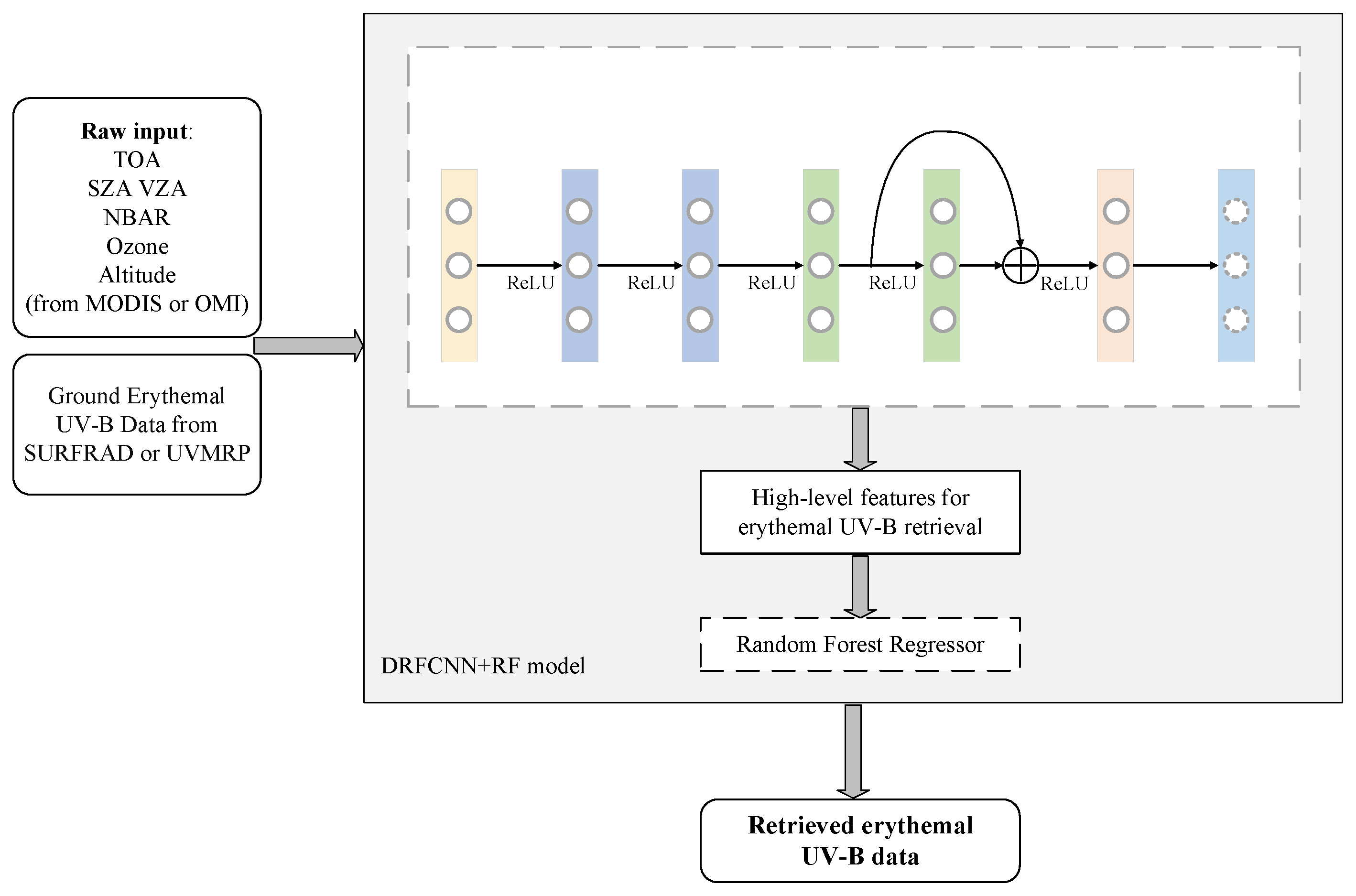
MODIS TOA reflectance data contain atmospheric and surface information. Therefore, we can directly establish the relationship between MODIS TOA and erythemal UV-B without additional satellite products or LUTs retrieving atmospheric parameters. Because we avoid obtaining atmospheric parameters, it may be challenging to establish a relationship between MODIS TOA and surface erythemal UV-B using a simple ML algorithm. Therefore, we propose a DNN-based erythemal UV-B retrieval framework for MODIS data. The proposed framework has two parts:
  • Deep feature extraction: The first part is a deep residual fully connected network (DRFCN), which converts MODIS TOA and other parameters in a data-driven manner into a representation that is more meaningful to the surface erythemal UV-B retrieval. The proposed DRFCN, while implementing progressive data distillation through these layers, uses the residual links to fuse the data refined from the shallow network. In addition, the residual connections construct short-cuts for gradient propagation, which leads to more stable training dynamics than simple feedforward networks. Finally, we obtain the best data representation for erythemal UV-B retrieval, which we call the deep feature.
  • Random forest regressor: After the deep features are extracted from the pre-trained residual network, they are used to fit an external RFR, a robust decision tree-based ensemble model to obtain the final predicted erythemal UV-B value. Although each depth feature of the RF input in the proposed method cannot point out the specific physical meaning, they are another manifestation of these parameters with specific physical significance.
The overall framework of the proposed algorithm is illustrated in Figure 2. The two parts of this framework can also be regarded as two deformed “LUT”s. The first “LUT” converts the MODIS TOA, surface reflectance, SZA, VAA, altitude, and total ozone column into other data representations (i.e., deep features) that are more relevant to surface erythemal UV-B retrieval. These expressions include not only the atmospheric parameter information output by the first LUT in the LUT algorithm but also the parameter information input in the second LUT in the algorithm. The second “LUT” establishes the relationship between these deep features and the surface erythemal UV-B and predicts the final surface erythemal UV-B data. This step has the same function as the second LUT in the algorithm, except that each parameter of the second LUT input has a physical meaning. Although each depth feature of the second “LUT” input in the proposed method cannot identify the specific physical meaning, they are another manifestation of these parameters with specific physical significance.

Deep Residual Fully Connected Network (DRFCN)

Theoretically, when the FCNN goes deeper, the features extracted by the network are more abstract and have greater generalization ability. However, there are two main problems in practice: (1) As the number of layers increases, gradient vanishing/exploding and network degradation may occur after the network depth exceeds a particular value. Network degradation refers to the phenomenon in which an increase in the number of network layers leads to saturated or decreased accuracy in the training set. (2) In addition, for FCNN, the information lost in previous layers could never be recovered, and the final decision made by FCNN was only based on the features from the last layer. However, it has been shown in previous work [57] that features from all abstract levels could be beneficial because they depict the raw inputs from different granularities.
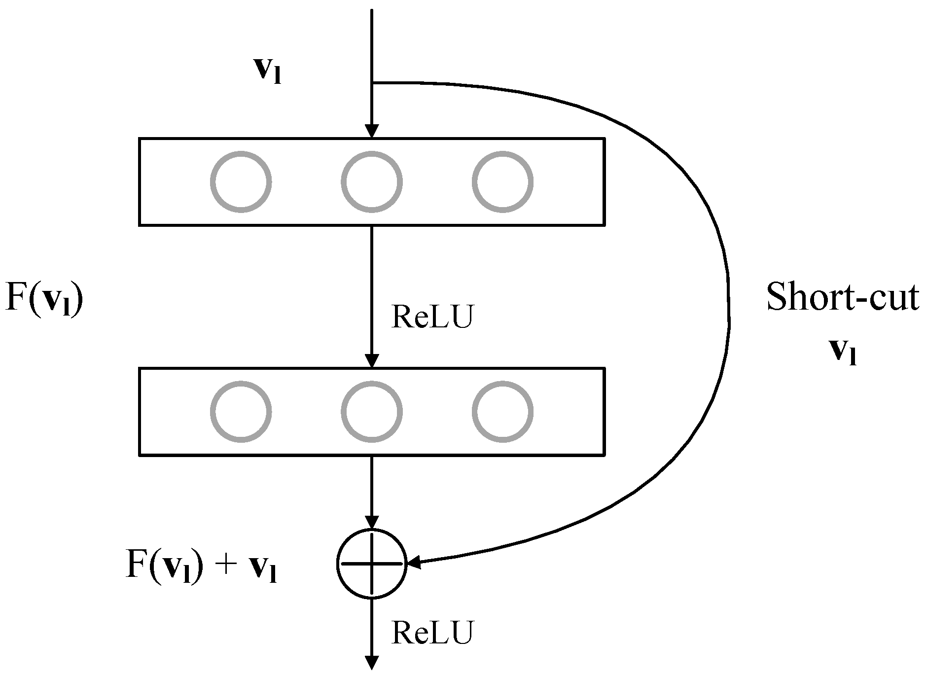
Therefore, we decided to use shortcut connections to construct residual blocks (Figure 3) to solve the above problems, where the deep features are refined in a cascading manner. Through shortcuts, the relationship between the input and output of each residual block can be expressed as:
v l + 1 = v l + F ( v l , W l )
where v l and v l + 1 are the input and output of the residual block, respectively, and F ( v l , W l ) is the residual mapping, which can be viewed as a refined term that fuses more abstract representations into the original v l .
In addition to its ability to alleviate the gradient vanishing/exploding and network degradation problems, the significant advantage of utilizing a residual network for erythemal UV-B retrieval is that the information can be smoothly propagated from the shallow layer to the deep layer by short-cut connections [58]. In a residual network, the short-cut connections directly fuse the shallow features into more abstract features obtained from the deep layers, which can be beneficial for erythemal UV-B retrieval, as features from all levels are comprehensively considered.

4.3. Benchmark Model Combination for Comparison

4.3.1. Ablation Study: FCNN, DRFCN, FCNN+RF, and DRFCN+RF

In the ablation study of the DRFCN+RF model, we removed a section of the model network to form a new model to validate its effectiveness. We obtained four models: FCNN, DRFCN, FCNN+RF, and DRFCN+RF. We evaluate and compare these four models on the dataset to determine whether the three sections of the FCNN, residual connections, and RF contributed to the performance of the model, proving that there are no redundant components in the DRFCN+RF model.

4.3.2. Method Intercomparison: SVR, RF, DRFCN+SVR, and DRFCN+RF

In method intercomparison, we compare the DRFCN+RF model with the classic RF and SVR. Both RF and SVR models are commonly used and well-performing ML methods for surface radiation flux estimation [31]. In addition, replacing RF in the DRFCN+RF model with SVR constitutes the DRFCN+SVR model, which is used for comparison.

4.4. Dataset

We established a new all-sky erythemal UV-B retrieval dataset D : p 1 i , , p K i , m i i r a n g e ( 1 , N ) . Each element in D has two components: the measured erythemal UV-B irradiance m and the corresponding parameters p = { p 1 , , p K } . In the dataset, we collected ground measurements of erythemal UV-B for 37 stations in the United States from 2007 to 2017 as the true value of the model (m in dataset D ). The parameters p are primarily obtained from MODIS and OMI products, including TOA reflectance (Band1–36), SZA and VZA from the MODIS level 1 product, surface reflectance data from MODIS MCD43A4 (Band1–7), total ozone column data from the OMI OMTO3d product, and the altitude of the station. These data obtained from satellite products and ground stations are directly used as the input of the DRFCN+RF model and benchmark models.
As demonstrated by Calbó et al. [16], the UV radiation reaching the ground is affected by many factors, including SZA, ozone, aerosol, cloud, altitude, and surface reflectance. The TOA reflectivity of MODIS can capture the temporal and spatial variations of clouds and aerosols, and combined with the ozone data from OMI, these two sets of parameters indicate the atmospheric conditions.
To verify the effectiveness of the proposed algorithm, we divided the dataset into three different subsets: SURFRAD, SURFRAD-2017, and UVMRP. The data from January 2007 to December 2016 in SURFRAD (19,655 samples) were randomly divided into three parts: 80 % was used for model training (15,723 samples), 10 % was used for model validation (1966 samples), and 10 % was used for model testing (1966 samples). SURFRAD-2017 (1801 samples) contained only SURFRAD data in 2017. UVMRP (43,395 samples) contains data from the 30 UVMRP sites from January 2007 to December 2016. Note that the sunny or cloudy data are not eliminated in the dataset. Therefore, the dataset we collected contains all-sky information.

4.5. Evaluation Strategy

According to the three parts of the dataset (SURFRAD, SURFRAD-2017, and UVMRP), the experiment can also be divided into three parts.
The SURFRAD dataset was used for models construction (model training, validation, and testing). We conducted three experiments on this data set: the influence of parameter combination on the DRFCN-RF model performance, ablation study of the DRFCN+RF model, and comparison against the baseline methods. Although we include various parameters in our dataset based on theoretical analysis, the parameter combination is far from optimal because the information of some parameters may overlap, which may lead to network redundancy. Therefore, to ensure that the proposed model and the subsequent classic ML models (SVR and RF) have the best performance, it is essential to choose a simple but effective combination of parameters. After selecting the optimal set of parameters, all benchmark models (FCNN, DRFCN, FCNN+RF, SVR, RF, and DRFCN+SVR) in the ablation study and method intercomparison experiment were trained on the SURFRAD dataset and drawn compared with the DRFCN-RF model on the SURFRAD test set.
After training the DRFCN-RF model on the SURFRAD dataset, UVMRP and SURFRAD-2017 were primarily used to verify the generalization ability of the DRFCN-RF model for temporal and spatial variation. The samples in the UVMRP and SURFRAD-2017 datasets never appear in the training set of SURFRAD dataset.

4.6. Evaluation Metrics

The models were evaluated using several statistical metrics, including M B E , n M B E , R M S E , n R M S E , R 2 , R, N S D , and N R M S D . The descriptions and formulas of these indicators are as follows.
Mean bias error ( M B E ) and normalized mean bias error ( n M B E ):
M B E = i = 1 N E i M i N
n M B E ( % ) = 100 M a v e i = 1 N E i M i N
The root-mean-square error ( R M S E ) and normalized root-mean-square error ( n R M S E ):
R M S E = i = 1 N E i M i 2 N
n R M S E ( % ) = 100 M a v e i = 1 N E i M i 2 N
Coefficient of determination ( R 2 ):
R 2 = i = 1 N E i M a v e 2 i = 1 N M i M a v e 2 = 1 i = 1 N M i E i 2 i = 1 N M i M a v e 2
Coefficient of correlation (R):
R = i = 1 N E i E a v e M i M a v e i = 1 N M i M a v e i = 1 N E i E a v e
The normalized standard deviation ( N S D ):
N S D = i = 1 N E i E a v e i = 1 N M i M a v e
The normalized centered root-mean-square difference ( N R M S D ):
N R M S D = N i = 1 N E i E a v e M i M a v e 2 i = 1 N M i M a v e
where E i is the estimated erythemal UV-B irradiance (i represents a number), M i is the ground measurements, M a v e the ground measurement average, E a v e is the estimated measurement average, and N is the number of all samples in the test set.
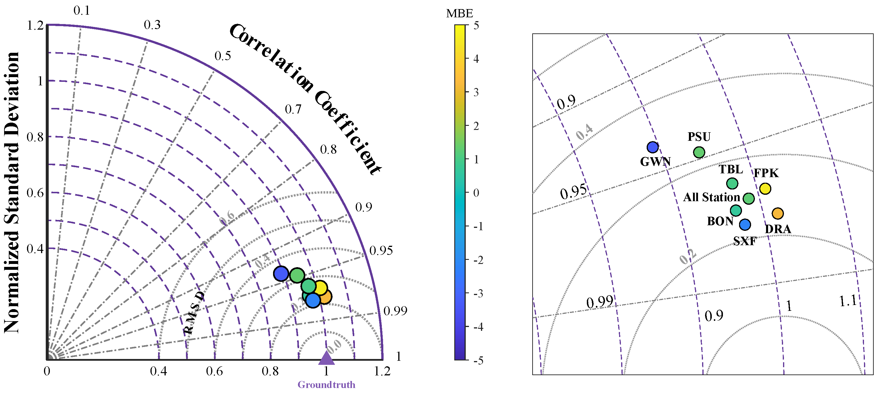
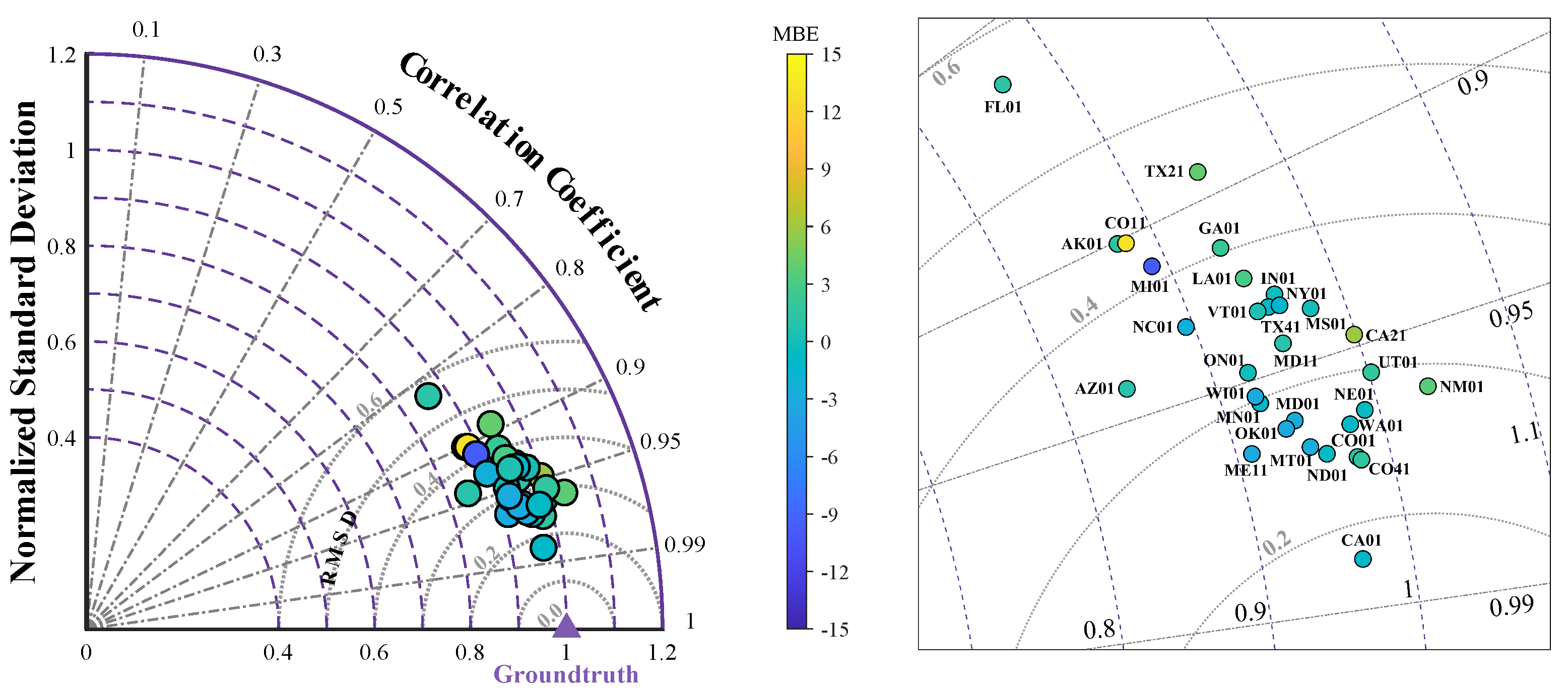
R, N S D , and N R M S D are used to draw the Taylor diagram [59,60], which evaluates the degree of closeness between the predicted erythemal UV-B and the ground observations in a graphical manner. In the Taylor diagram, the cosine of polar angles represents R, the values of the x-axis and y-axis represent N S D , the radius from the ground truth point represents N R M S D , and the expectation point is located on the x-axis at unit distance. Three parameters, R, N S D , and N R M S D , determine the position of the point in the Taylor diagram and represent the overall predicted erythemal UV-B values. Moreover, the closer the point is to the ground truth point, the more reliable the predicted erythemal UV-B values.

5. Comparison Results

5.1. Evaluation on SURFRAD Test Set

5.1.1. Parameter Sensitivity Analysis

To determine the best model input for erythemal UV-B estimation, different parameter combinations were considered in the proposed DRFCN+RF model. The initial parameters include TOA reflectance, SZA, VZA, VAA, SAA, altitude, latitude, ozone, and surface reflectance. The compositions of these parameters and corresponding results of the models are listed in Table 2.
From Table 2, we can see that the model with inputs composed of “TOA reflectance + SZA + VZA + ozone + altitude + surface reflectance” performs best. When SZA, VZA, and altitude already exist in the parameter combination, the accuracy of the model is not significantly improved when latitude, SAA, and VAA are included. The reason for this could be that the additional parameters SZA, VZA, RAA, SAA, VAA, altitude, and latitude overlap, which introduces more trainable parameters in the network but provides less extra information, making the network prone to overfitting. We finally chose SZA, VZA, and altitude as the input parameters. The ozone parameter provides information on the concentration of ozone in the atmosphere. The surface reflectance parameter can distinguish different surface types and is essential for erythemal UV-B retrieval when snow cover is present at high latitudes. The parameter combination of “TOA reflectance + SZA + VZA + ozone + altitude + surface reflectance” will be the default setting for all subsequent experiments regarding erythemal UV-B retrieval, unless specified otherwise.

5.1.2. Ablation of DRFCN+RF Model

The performance of the DRFCN+RF model and the three baselines (FCNN, DRFCN, and FCNN+RF) were evaluated on the SURFRAD test set, and Table 3 summarizes their results. In Table 3, the data marked in red are the optimal results for each statistical metric.
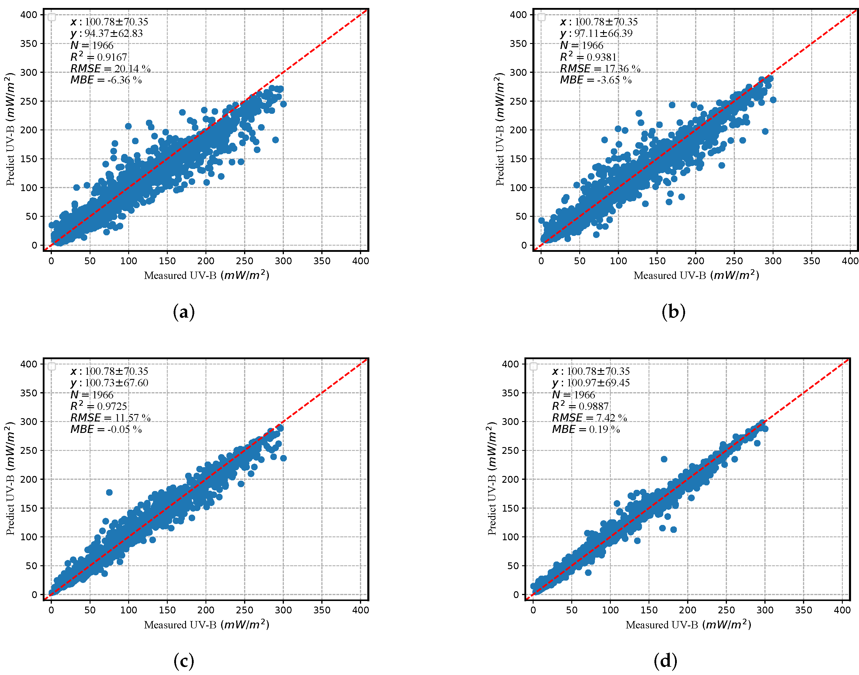
Compared with the FCNN ( R 2 = 0.9167 , R M S E = 20.14 % ), DRFCN ( R 2 = 0.9381 , R M S E = 17.36 % ), and FCNN+RF ( R 2 = 0.9725 , R M S E = 11.57 % ) models, the DRFCN+RF ( R 2 = 0.9887 , R M S E = 7.42 % ) model can achieve the maximum R 2 and the lowest R M S E for erythemal UV-B retrieval at seven SURFRAD stations, as shown in Table 3 and Figure 4.
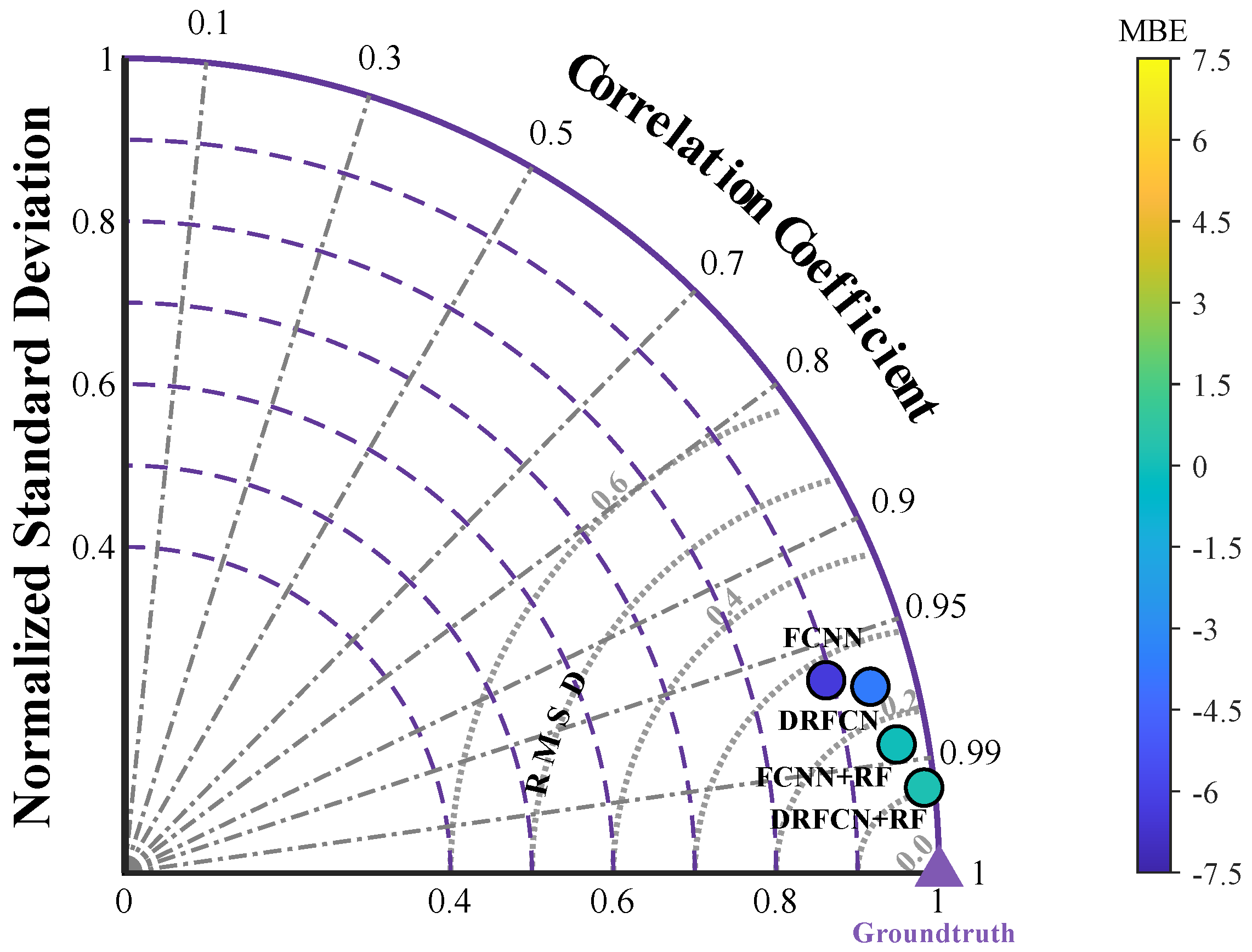
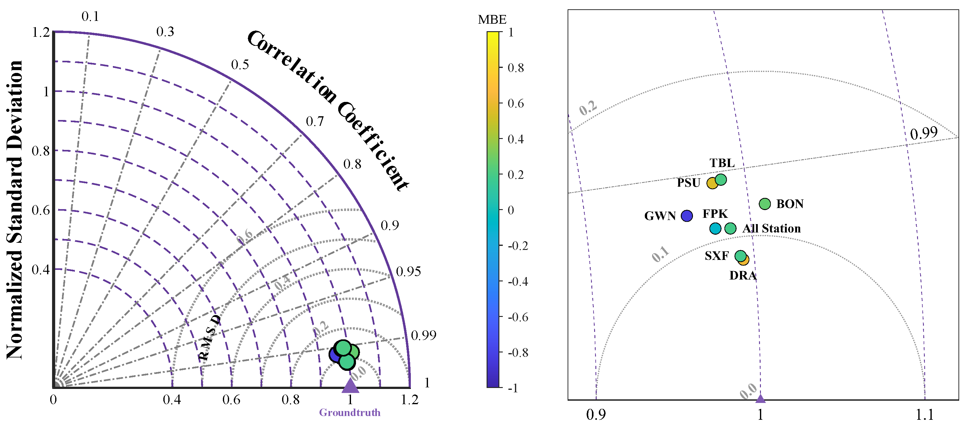
To intuitively demonstrate the contribution of each part of the model to the predicted results, the four parameters R, N S D , R M S D , and M B E in Table 3 are used to draw the Taylor diagram shown in Figure 5. The N S D of all four models is less than 1, indicating that these models underestimate the amplitude of the surface erythemal UV-B irradiance cycle found in the ground observations. However, the degree of underestimation of DRFCN+RF was the smallest among the four methods, and its N S D value was approximately equal to 1. The proposed DRFCN+RF model was close to the ground truth point, which confirms that the forecasting accuracy was significantly higher than the other three compared models in the ablation study. It is shown that the FCNN, DRFCN, and FCNN+RF models are not appropriate because the model points are highly parted from the ideal observed point. After adding the residual connection (FCNN vs. DRFCN, FCNN+RF vs. DRFCN+RF) or introducing RF (FCNN vs. FCNN+RF, DRFCN vs. DRFCN+RF), the model after introducing other structures is closer to the ground truth point than the previous model. However, when we compare the degree of distance improvement, we find two points. First, the distance difference between the FCNN and DRFCN models to the ground truth point is less than that between the FCNN+RF and DRFCN+RF models to the ground truth point. When RF is included in the model, the addition of the residual connection improves the final erythemal UV-B prediction accuracy. Secondly, the distance difference between the FCNN and FCNN+RF models to the ground truth point is smaller than the distance between the DRFCN and DRFCN+RF models to the ground truth point. In other words, RF can improve the effects of the model based on the existing part of the residual connection. The residual connection improves the model even more when used in combination with RF.
The following conclusions can be drawn: The DRFCN+RF framework proposed in this paper is helpful in erythemal UV-B retrieval. Both the residual connection and RF components can significantly improve the accuracy of the final predicted value of erythemal UV-B. There are two primarily explanations for this result: First, the residual connection refines high-level features from low-level features. The shortcuts constructed by the residual connection are transferred by a gradient, which stabilizes the optimization of the model. In addition, the RF can obtain more reliable regression results and cannot easily fall into overfitting because of its multi-decision tree characteristics and the use of the bagging algorithm. Furthermore, combined with the residual connection, the dataset entered into the RF is not the raw data but the deep features that are refined from raw data; thus, the combination of the two will produce a better effect.

5.1.3. Method Inter-Comparison

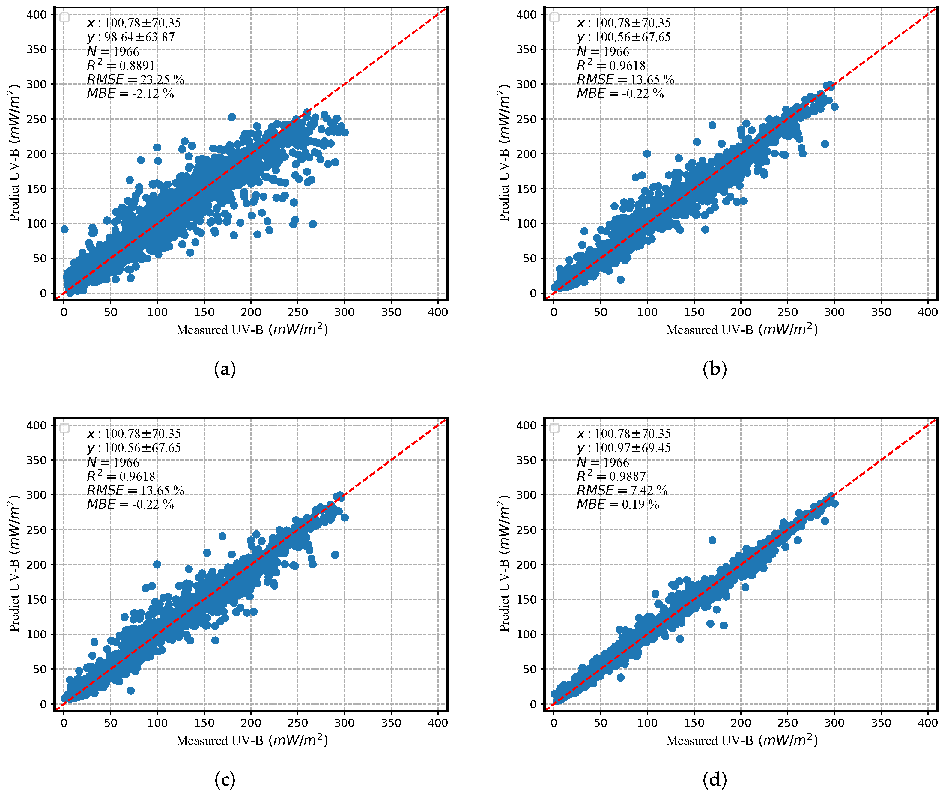
Table 4 summarizes the performance comparison between the proposed DRFCN+RF model and the baselines (RF, SVR, and DRFCN+SVR). The data marked in red are the best results for each statistical metric. Under the two sets of statistical indicators, the optimal model for each site was the DRFCN+RF model proposed in this study. It can also be seen from the scatter diagram in Figure 6 and subgraphs (Figure 6a–d) that the scatter gradually approaches the ideal position, as illustrated by the red dotted line. As for Figure 6d, almost all points are close to the red line and its vicinity, and only a few points deviate from the ideal position. However, the degree of deviation is smaller than that of the previous three subgraphs. Compared with the SVR, RF, and DRFCN+SVR models, the R M S E of the DRFCN+RF model ( R M S E of 7.42 % ) decreased by 16 % , 12 % , and 6 % , respectively; the R 2 of the DRFCN+RF model (0.9887) and the R M S E of the DRFCN+RF model ( R M S E is 7.42 % ) has an average improvement of 11 % , 8 % , and 3 % , respectively.
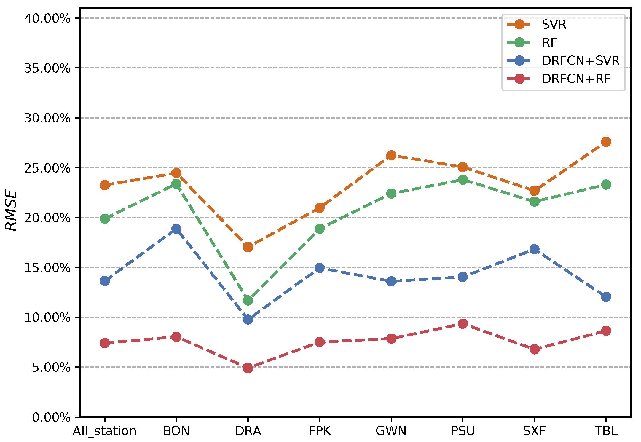
A further diagnostic test was performed using a line graph (Figure 7) based on R M S E . Note that the objective of this section is to evaluate the performance of each model at each station. First, we found that all four methods on DRA, SXF, and FPK performed better than the other four stations. As mentioned in Section 5.1.4, DRA, FPK, and SXF are in a dry, sunny climate with less extreme weather, which is very conducive to erythemal UV-B value retrieval due to the environmental superiority of the station itself. Most importantly, compared to SVR, RF, and FCNN, the DRFCN+RF model had the smallest change in R M S E at the seven sites. The difference in the R M S E of the DRFCN+RF model on the seven sites did not exceed 4.5 % . In contrast, among the SVR, RF, and DRFCN+SVR models, these differences reached 9 % , 12 % , and 11 % , respectively. For the three baseline models, the site’s environment had a more significant impact on the model performance. The DRFCN+RF model is the most robust regarding the impact of the site environment on erythemal UV-B retrieval. The R, N S D , and N R M S D data in Table 4 also confirm that the accuracy of the model at all seven stations is significantly higher than that of the other three comparison models. Further verification of the robustness of the model is presented in Section 5.3.

5.1.4. Evaluation of DRFCN+RF Model

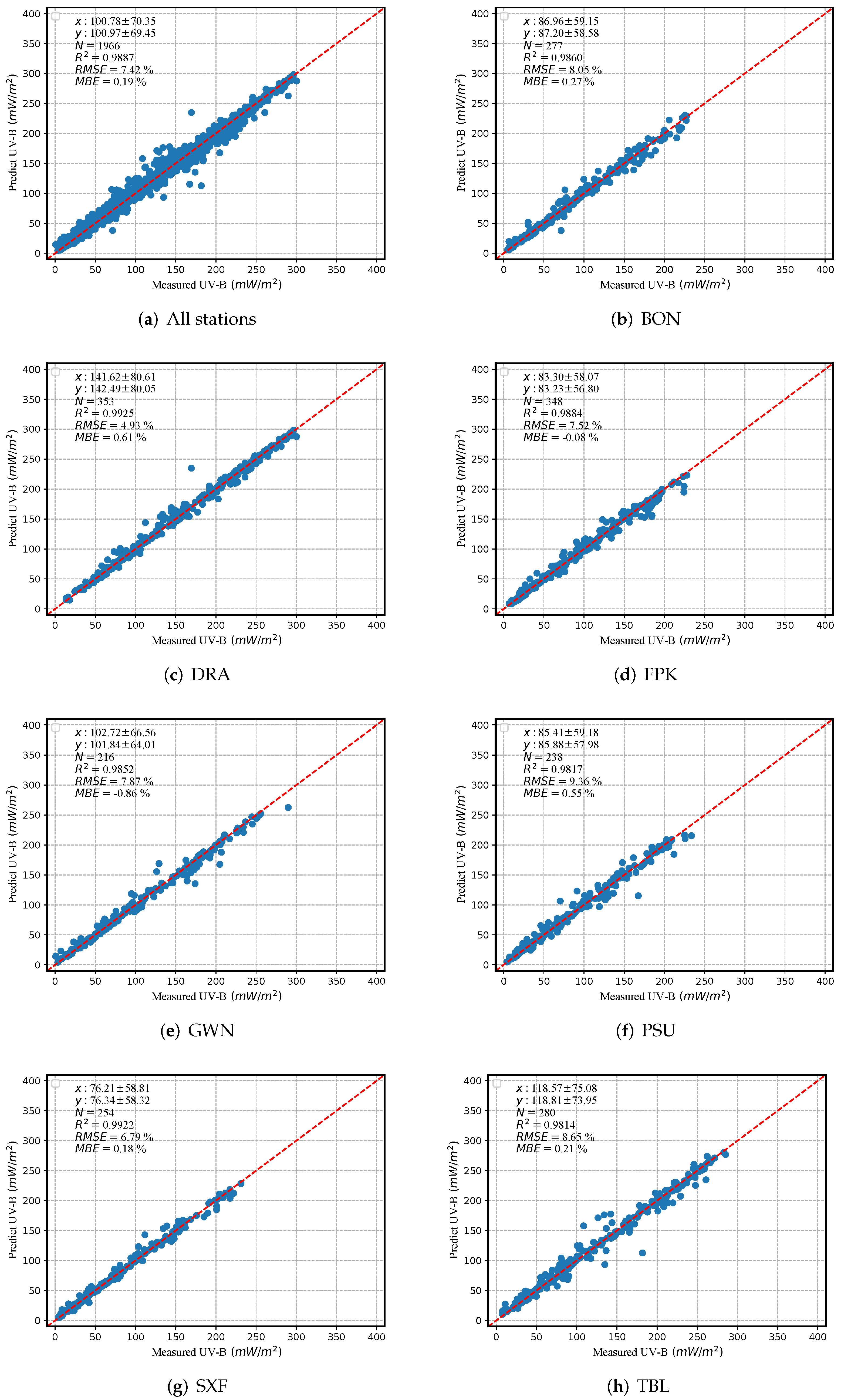
In this section, we further show the evaluation results of DRFCN+RF on the seven SURFRAD sites. The values of the R 2 , M B E , and R M S E of the entire SURFRAD test set generated by the DRFCN+RF model are as follows: R 2 = 0.9887 , M B E = 0.19 mW/m 2 ( 0.19 % ), and R M S E = 7.48 mW/m 2 ( 7.42 % ). Figure 8 shows the scatterplot between the ground measurements and the estimated erythemal UV-B at seven SURFRAD stations. From the relative relationship between the points in the scatterplot and the red dotted line, with the specific data in Table 5, we draw the same conclusion as in Section 5.1.3: DRA with a hot arid climate and the SXF and FPK stations in the northern plains perform better.
Although the proposed model performs best at the DRA, SXF, and FPK, the evaluation results of the seven stations are very similar. Seven stations had R 2 values ranging from 0.9814 (TBL) to 0.9925 (DRA), R M S E varying from 4.92 % (DRA) to 9.36 % (PSU), and the M B E remained below ± 1 % . These two results are displayed more clearly in the Taylor diagram shown in Figure 9. In the Taylor diagram, the eight circles are all very close to the ground truth point. Therefore, the accuracy of the estimated erythemal UV-B values obtained by the DRFCN+RF model at each SURFRAD station was at the same level.
After a step-by-step verification in Section 5.1.2, Section 5.1.3 and Section 5.1.4, the following conclusions can be drawn: The DRFCN+RF model is a well-designed and practical model for surface erythemal UV-B retrieval from raw MODIS data. First, the model consistently outperformed models based on single ML or single deep learning by a large margin. This is not only reflected in the performance of the DRFCN+RF model on the test set being optimal under various precision evaluation indices but also in the accuracy difference of the estimated erythemal UV-B value obtained by each SURFRAD station under the DRFCN+RF model being the smallest. In addition, all parts of the DRFCN+RF model are valid, and some parts contribute positively to improve the accuracy.

5.2. Model Evaluation with SURFRAD-2017 Dataset

For the SURFRAD-2017 dataset, the model evaluation results for each station are summarized in Table 6. The SURFAD dataset used in Section 5.1 collected data from 2007 to 2016, while the SURFRAD-2017 dataset used in this section was only collected in 2017. Although the data of these two datasets are all from seven SURFRAD stations, none appear in the training set, which can be used to demonstrate the model’s robustness towards temporal differences.
As shown in Table 6, the model performs best on the SURFRAD-2017 dataset at DRA, SXF, and FPK. Seven stations have R 2 values ranging from 0.8966 (GWN) to 0.9515 (SXF), R M S E s from 12.95 % (DRA) to 20.95 % (FPK), and M B E s that remain below ± 5 % . The values of the R 2 , M B E , and R M S E on the entire SURFRAD-2017 of the DRFCN-RF model are R 2 = 0.9367 , M B E = 1.24 mW/m 2 ( 1.27 % ), and R M S E = 17.45 mW/m 2 ( 17.88 % ). Compared with the performance of the model on the SURFRAD test set in Section 5.1.4, ( R 2 = 0.9887 , M B E = 0.19 mW/m 2 ( 0.19 % ) and R M S E = 7.48 mW/m 2 ( 7.42 % )), the R-value decreases, and the R M S E and M B E values increase.
To visualize the difference between the model performance on the SURFRAD test set and the SURFRAD-2017 dataset, the R, N S D , and N R M S D data in Table 6 were used to draw the Taylor diagram shown in Figure 10. This is compared with Figure 9, which represents the SURFRAD test set. The N S D data change little on the two datasets, indicating that the model can estimate the surface erythemal UV irradiance period amplitude found in ground observations. The movement of SURFRAD-2017 points in the opposite direction to the ground truth point, compared with the SURFRAD points, may be caused by the interannual variation of ground station data. Nevertheless, this moving distance is maintained within an acceptable range, which proves the robustness of the model. However, the comparison of the metrics obtained by the model in the SURFRAD-2017 dataset and the SURFRAD dataset is more indicative of the ability of the model to “predict” erythemal UV-B values. Therefore, the validation of the model robustness will be more rigorously demonstrated in the next section using the UVMRP dataset.

5.3. Model Validation against UVMRP Dataset

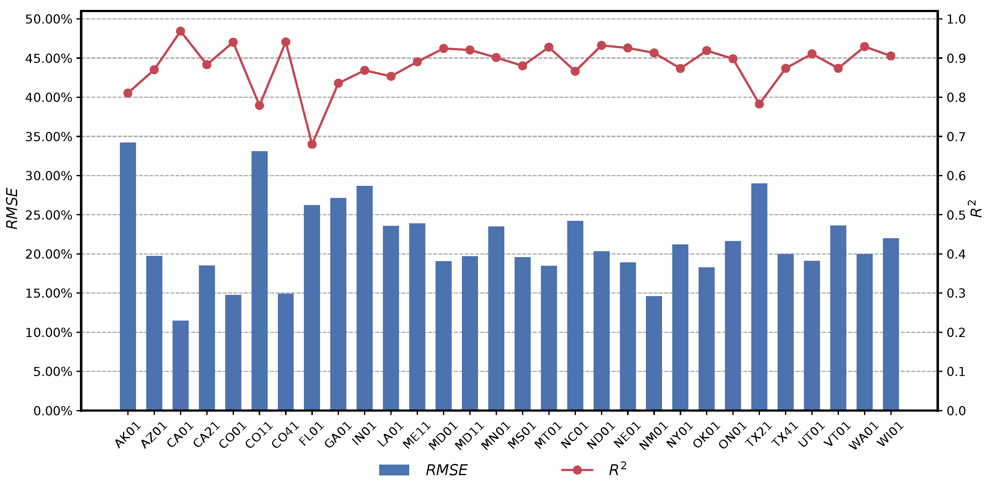
In this section, the UVMRP dataset is used to verify the robustness of the DRFCN+RF model in different environments. Table 7 summarizes the performance of the model for the UVMPR stations. With the exception of the site in Steamboat Springs, Colorado (CO11), where the M B E value was 12.96 % , the rest had M B E values within the range of ± 5 % . The R 2 and R M S E parameters in Table 7 are plotted in Figure 11. When using the R M S E evaluation model, the R M S E values of most UVMRP stations were below 25 % . Most sites had an R 2 value of approximately 0.9.
To visualize the model performance, each UVMRP site was plotted in a Taylor diagram (Figure 12) by R, N S D , and N R M S D to provide a holistic and detailed assessment. Figure 12 shows that 28 out of 30 stations (93%) had an R above 0.9 and n M B E   ±   5 % , N S D values range from 0.8 to 1.1, and R M S D values ranged from 0.18 (CA01) to 0.56 (FL01). It is evident that the site in Homestead, Florida (FL01), had the worst estimations in R ( 0.8258 ), N S D ( 0.8620 ), and R M S D ( 0.56 ). This is due to the severe air pollution in the southeastern region of the United States, where FL01 is located, and the high humidity of the tropical climate leads to daily cloud accumulation. The same factors also exist at the sites in LA01 ( R M S E = 23.56%), GA01 ( R M S E = 27.12%), and MS01 ( R M S E = 19.58%). TX21 ( R M S E = 28.98%) and TX41 ( R M S E = 19.99%) have N R M S D value of 0.46 and 0.36, respectively, likely due to local air pollution and possible pollution transfer from Mexico. IN01 ( R M S E = 28.67%) and MN01 ( R M S E = 23.48%) in the Midwest, and ME11 ( R M S E = 23.87%), ON01 ( R M S E ), and VT01 ( R M S E = 23.61%) in the northeast also showed higher bias and N R M S D values due to regional air pollution. Additionally, sites in Fairbanks, Alaska (AK01), and Steamboat Springs, Colorado (CO11), all had relatively larger N R M S D s (both 0.43). CO11 ( R M S E = 33.08%) is a high-altitude site (3220 m above sea level), and AK01 ( R M S E = 34.19%) is approximately 2 degrees south of the Arctic Circle and is the northernmost site in the UVMRP. The geographical location of both results in a low erythemal UV-B value collected at the two sites, which causes the N R M S D value to move in the opposite direction of the groundtruth point. In particular, cloud changes and local turbulence at the top of the Rocky Mountains are crucial for high N R M S D and M B E phenomena at the CO11 site. In comparison, sites in the north, the Rocky Mountains, and the Central Plains have smaller N R M S D s, such as ND01, MT01, WA01, NE01, ME11, CO01, CO41, etc. In addition, a small R M S E can be found from the southwest stations such as NM01 and CA01. Furthermore, the site in Davis, California (CA01), shows the best estimation with R = 0.9845 , the N R M S D = 0.18 , and the R M S E = 11.47 % . CA01 is located in the desert, with sufficient sunlight and low air pollution, which is significant for the excellent performance of the model at this site.
The spatial variability of erythemal UV-B retrieval accuracy from MODIS found in our DRFCN+RF model is consistent with the study of Zhang et al. [61], which evaluated OMI level 2 UV-B data at satellite overpass time with ground measurements at 30 UVMRP stations throughout 2005 to 2017. However, the performance of OMI on various sites is generally worse than that of DRFCN. The evaluation results of Zhang et al. [61] showed that the N R M S D varies from 0.34 (CA01) to 0.71 (FL01), the n M B E from 0.54% (NC01) to 24.5% (FL01), and 12 out of 30 sites (38%) had R below 0.9. Although FL01 has always been the worst performance point, the performance of DRFCN+RF using MODIS on this site (R = 0.8258, n M B E = 1.19%, N R M S D = 0.56) compared with its performance on OMI (R = 0.74, n M B E = 24.5%, N R M S D = 0.71) has a greater improvement. The same is true on the best performing site CA01 (OMI: R = 0.95, N R M S D = 0.34; DRFCN+RF: R = 0.9845, N R M S D = 0.18).
There are regional differences in the performance of the DRFCN+RF model, and the model performs better when the air is dry and it rains less. However, at most stations, the proposed method provides reasonable estimates. Compared to the SURFRAD sites, the results for N R M S D increased slightly, but the M B E values remained at the same level for almost all UVMRP sites.

5.4. Discussions

In the experiments, we have evaluated the proposed DRFCN+RF under two different settings to demonstrate its superior effectiveness compared to other methods. Specifically, we focus on the UV-B retrieval ability and generalization ability of Different UV-B retrieval strategies, of which we will discuss in the following subsections. Moreover, we discuss the broader impacts in the last sub-section.

5.4.1. UV-B Retrieval Ability of Different Algorithms

In the first setting, the common evaluation strategy is adopted where the models are trained and tested on the same stations. We found that all models performed better on the three dry and less rainfall stations (DRA, SXF, and FPK). The performance of the DRFCN+RF model is consistent among the seven sites, while the performance of machine learning and fully connected networks varies significantly between sites. This demonstrate that traditional statistical methods may present limited ability for discerning the complex relationship between high-resolution MODIS, atmospheric surface products (i.e., TOA reflectance, SZA, view zenith angle (VZA), and surface reflectance), and erythemal UV-B levels.
From the experimental results, we can find that the proposed DRFCN+RF is consistently better than shallow machine learning methods and the vanilla fully connected networks. This demonstrates that the proposed cascade feature refinement module of DRFCN is indeed a suitable and advanced feature extraction strategy for UV-B retrieval tasks. In addition, with an RF classifier introduced as the post-processing module, the performance of DRFCN+RF can be further improved with a modest extra computational budget, which justifies the two-stage modeling strategy of the proposed DRFCN+RF model.

5.4.2. Generalization Ability of DRFCN+RF

In the second setting, we train the models on SURFRAD stations and test them on other stations. Since the data distribution from the training set may be different from that of the testing set, this setting is consistently more difficult compared with the first one. We conduct experiments on this setting to demonstrate the generalization ability of the proposed DRFCN+RF. In addition, we compare the validation results of the OMI level 2 swath products and DRFCN+RF model at 30 UVMRP sites [61]. Under the exact estimation of the instantaneous UV-B at satellite overpass time, the performance of the DRFCN+RF model is better than OMI at each site. Among them, the N R M S D of DRFCN+RF is about 0.16 lower than OMI. In the DRFCN+RF model, 28 sites have an R more significant than 0.9, and 14 sites have an R above 0.95. However, only 19 sites in OMI have an R more significant than 0.9 and no more than 0.95. This comparison further illustrates that the DRFCN+RF model has relatively strong robustness.
The experimental results show that DRFCN+RF trained on SURFRAD station can indeed have satisfactory performance when evaluated on UVMRP stations, which demonstrates that the DRFCN+RF model has better spatial generalization capabilities.

5.4.3. Broader Impact of DRFCN+RF

The proposed methods can be generalized to other retrieval tasks where the mapping from the parameters to the retrieval target is complex and can benefit from a cascaded feature refinement via the residual network, such as Surface net radiation retrieval and downward shortwave radiation retrieval. The only change to our framework is to adjust the network input and output to make them compatible to the data of the new retrieval task. Therefore, we speculate that the proposed DRFCN+RF can have a broader impact on remote sensing tasks other than UV-B retrieval in this paper.

6. Conclusions

In this paper, we propose a robust DL model (DRFCN+RF) to retrieve all-sky erythemal UV-B from 1 km MODIS TOA data with the support of ancillary ozone information. Specifically, DRFCN+RF adopts the residual connection structure designed to refine the raw MODIS features in the neural network, and an external RF post-processing module is used to perform the final prediction of erythemal UV-B based on the refined deep features.
In the sensitivity analysis, we selected “TOA reflectance + SZA + VZA + latitude + ozone + surface reflectance” as the default setting for all subsequent experiments. To evaluate the model performance, we compared DRFCN+RF with six baseline models (FCNN, FCNN+RF, DRFCN, DRFCN+SVR, RF, and SVR) on the SURFRAD test dataset. Evaluation on the SURFRAD test set demonstrates that the proposed model achieves an R 2 of 0.9887, an M B E of 0.19 mW/m 2 ( 0.19 % ), an R M S E of R M S E = 7.48 mW/m 2 ( 7.42 % ), an N S D of 0.9872 , and an N R M S D of 0.11, which is the best among all the tested methods. A comparison of the three baselines in the ablation study (FCNN, DRFCN, and FCNN+RF) shows that both the residual connection and the RF post-processing module in the DRFCN+RF can significantly improve the accuracy of the final predicted value of erythemal UV-B. Compared with the classic ML models RF, SVR and FCNN, the R M S E value of the DRFCN+RF model decreased by 12.46%, 15.83%, and 12.72%, respectively.
Furthermore, considering the performance of the model at 37 stations (7 stations in the SURFRAD dataset and 30 stations in the UVMRP dataset), the M B E of 35 stations was within ± 5 % , 32 stations ( 86 % ) had R 2 values above 0.85, and 31 stations ( 84 % ) had R M S E values below 25 % . Therefore, the model has good generalization ability. However, there are some regional differences in the performance of the DRFCN+RF model, and it performs better when the air is dry and rain-less. By evaluating the model performance on the UVMRP dataset, the model can be proven to be a powerful model for ground erythemal UV-B retrieval based on MODIS data.
This paper demonstrates the great potential of using MODIS data to accurately estimate all-sky instantaneous erythemal UV-B with the proposed deep learning algorithm. The much-improved spatial resolution achieved by our MODIS UV-B estimation may allow for more downstream applications in the future.

Author Contributions

Conceptualization, T.H.; methodology and experiments, R.Z.; writing—original draft preparation, R.Z.; writing—review and editing, T.H. All authors have read and agreed to the published version of the manuscript.

Funding

This research was funded by the National Natural Science Foundation of China under Grant 42090012, the Hubei Natural Science Grant 2021CFA082, and the Fundamental Research Funds for the Central University through Wuhan University under Grant 2042021kf0203.

Data Availability Statement

The Ground measurements erythemal UV-B data in America were obtained from SURFRAD (https://gml.noaa.gov/grad/surfrad/, accessed on 31 November 2021) and UVMRP (https://uvb.nrel.colostate.edu/UVB/, accessed on 31 November 2021). The kilometer-level TOA, SZA, VAA, and SAA data were available from the product MODIS (https://www.giss.nasa.gov/, accessed on 31 November 2021). The OMTO3d data were obtained from OMI (https://disc.gsfc.nasa.gov/datasets/OMTO3d_003/summary?keywords=OMI%20O3&start=1920-01-01&end=2019-12-30, accessed on 31 November 2021).

Acknowledgments

The authors appreciate the comments and suggestions from the anonymous reviewers. We would also like to thank Jiang Chen for helping with the original draft preparation and data curation. We gratefully acknowledge data support from the National Earth System Science Data Center, National Science & Technology Infrastructure of China (http://www.geodata.cn, accessed on 31 November 2021).

Conflicts of Interest

The authors declare no conflict of interest.

Abbreviations

The following abbreviations are used in this manuscript:
MODISModerate resolution imaging spectroradiometer
UVUltraviolet
UV-BUltraviolet-B
TOATop-of-atmosphere
SZASolar zenith angle
VZAView zenith angle
SAASolar azimuth angles
VAAView azimuth angle
NBARNadir bidirectional reflectance distribution function-adjusted reflectance
CODCloud optical depth
AODAerosol optical depth
SURFRADSurface radiation budget network
UVMRPUV-B monitoring and research program
NDACCInternational network for the detection of atmospheric composition change
NOAANational oceanic and atmospheric administration
USDAUnited states department of agriculture
TOMS/EPTotal ozone mapping spectrometer onboard the earth probe satellite
OMIOzone monitoring instrument
GOME-2Global ozone monitoring experiment-2
TEMISTropospheric emission monitoring internet service
RTRadiative transfer
LUTLook-up-table
AVHRR/3Third advanced very high-resolution radiometer
CERNChinese ecosystem research network
MLMachine learning
SVMSupport vector machine
SVRSupport vector regression
RFRandom forest
RFRRandom forest regressor
ANNArtificial neural networks
GA-ANNGenetic algorithm-ANN
DLDeep learning
DNNDeep neural networks
FCNNFully connected neural network
DRFCNDeep residual fully connected network
M B E Mean bias error
n M B E Normalized mean bias error
R M S E Root mean square error
n R M S E Normalized root-mean-square error
R 2 Coefficient of determination
RCoefficient of correlation
N S D Normalized standard deviation
N R M S D Normalized centered root-mean-square difference

References

  1. Gray, L.J.; Beer, J.; Geller, M.; Haigh, J.D.; Lockwood, M.; Matthes, K.; Cubasch, U.; Fleitmann, D.; Harrison, G.; Hood, L.; et al. Solar influences on climate. Rev. Geophys. 2010, 48. [Google Scholar] [CrossRef]
  2. Singh, S.; Lodhi, N.K.; Mishra, A.K.; Jose, S.; Kumar, S.N.; Kotnala, R. Assessment of satellite-retrieved surface UVA and UVB radiation by comparison with ground-measurements and trends over Mega-city Delhi. Atmos. Environ. 2018, 188, 60–70. [Google Scholar] [CrossRef]
  3. Utrillas, M.; Marín, M.; Esteve, A.; Salazar, G.; Suárez, H.; Gandía, S.; Martínez-Lozano, J. Relationship between erythemal UV and broadband solar irradiation at high altitude in Northwestern Argentina. Energy 2018, 162, 136–147. [Google Scholar] [CrossRef]
  4. Holick, M.F. Biological effects of sunlight, ultraviolet radiation, visible light, infrared radiation and vitamin D for health. Anticancer Res. 2016, 36, 1345–1356. [Google Scholar]
  5. Serrano, M.A.; Cañada, J.; Moreno, J.C.; Gurrea, G. Solar ultraviolet doses and vitamin D in a northern mid-latitude. Sci. Total Environ. 2017, 574, 744–750. [Google Scholar] [CrossRef]
  6. Young, C. Solar ultraviolet radiation and skin cancer. Occup. Med. 2009, 59, 82–88. [Google Scholar] [CrossRef] [Green Version]
  7. Xiang, Y.; Laurent, B.; Hsu, C.H.; Nachtergaele, S.; Lu, Z.; Sheng, W.; Xu, C.; Chen, H.; Ouyang, J.; Wang, S.; et al. RNA m 6 A methylation regulates the ultraviolet-induced DNA damage response. Nature 2017, 543, 573–576. [Google Scholar] [CrossRef]
  8. Young, A.R.; Claveau, J.; Rossi, A.B. Ultraviolet radiation and the skin: Photobiology and sunscreen photoprotection. J. Am. Acad. Dermatol. 2017, 76, S100–S109. [Google Scholar] [CrossRef] [Green Version]
  9. Bernard, J.J.; Gallo, R.L.; Krutmann, J. Photoimmunology: How ultraviolet radiation affects the immune system. Nat. Rev. Immunol. 2019, 19, 688–701. [Google Scholar] [CrossRef] [PubMed]
  10. McKinlay, A.; Diffey, B. A reference spectrum for ultraviolet induced erythema in human skin. CIE J. 1987, 6, 17–22. [Google Scholar]
  11. Iqbal, M. An Introduction to Solar Radiation; Elsevier: Amsterdam, The Netherlands, 2012. [Google Scholar]
  12. Sola, Y.; Lorente, J.; Campmany, E.; De Cabo, X.; Bech, J.; Redaño, A.; Martínez-Lozano, J.; Utrillas, M.; Alados-Arboledas, L.; Olmo, F.; et al. Altitude effect in UV radiation during the Evaluation of the Effects of Elevation and Aerosols on the Ultraviolet Radiation 2002 (VELETA-2002) field campaign. J. Geophys. Res. Atmos. 2008, 113. [Google Scholar] [CrossRef] [Green Version]
  13. Wang, L.; Gong, W.; Luo, M.; Wang, W.; Hu, B.; Zhang, M. Comparison of different UV models for cloud effect study. Energy 2015, 80, 695–705. [Google Scholar] [CrossRef]
  14. Fountoulakis, I.; Bais, A.F.; Fragkos, K.; Meleti, C.; Tourpali, K.; Zempila, M.M. Short-and long-term variability of spectral solar UV irradiance at Thessaloniki, Greece: Effects of changes in aerosols, total ozone and clouds. Atmos. Chem. Phys. 2016, 16, 2493–2505. [Google Scholar] [CrossRef] [Green Version]
  15. Zempila, M.M.; Fountoulakis, I.; Taylor, M.; Kazadzis, S.; Arola, A.; Koukouli, M.E.; Bais, A.; Meleti, C.; Balis, D. Validation of OMI erythemal doses with multi-sensor ground-based measurements in Thessaloniki, Greece. Atmos. Environ. 2018, 183, 106–121. [Google Scholar] [CrossRef] [Green Version]
  16. Calbó, J.; Pages, D.; González, J.A. Empirical studies of cloud effects on UV radiation: A review. Rev. Geophys. 2005, 43. [Google Scholar] [CrossRef] [Green Version]
  17. Kim, J.; Cho, H.K.; Mok, J.; Yoo, H.D.; Cho, N. Effects of ozone and aerosol on surface UV radiation variability. J. Photochem. Photobiol. B Biol. 2013, 119, 46–51. [Google Scholar] [CrossRef]
  18. Renaud, A.; Staehelin, J.; Fröhlich, C.; Philipona, R.; Heimo, A. Influence of snow and clouds on erythemal UV radiation: Analysis of Swiss measurements and comparison with models. J. Geophys. Res. Atmos. 2000, 105, 4961–4969. [Google Scholar] [CrossRef]
  19. Augustine, J.A.; Hodges, G.B.; Cornwall, C.R.; Michalsky, J.J.; Medina, C.I. An update on SURFRAD—The GCOS surface radiation budget network for the continental United States. J. Atmos. Ocean. Technol. 2005, 22, 1460–1472. [Google Scholar] [CrossRef]
  20. Driemel, A.; Augustine, J.; Behrens, K.; Colle, S.; Cox, C.; Cuevas-Agulló, E.; Denn, F.M.; Duprat, T.; Fukuda, M.; Grobe, H.; et al. Baseline Surface Radiation Network (BSRN): Structure and data description (1992–2017). Earth Syst. Sci. Data 2018, 10, 1491–1501. [Google Scholar] [CrossRef] [Green Version]
  21. Liang, S.; Zheng, T.; Liu, R.; Fang, H.; Tsay, S.C.; Running, S. Estimation of incident photosynthetically active radiation from Moderate Resolution Imaging Spectrometer data. J. Geophys. Res. Atmos. 2006, 111. [Google Scholar] [CrossRef] [Green Version]
  22. Wang, D.; Liang, S.; Zhang, Y.; Gao, X.; Brown, M.G.; Jia, A. A New Set of MODIS Land Products (MCD18): Downward Shortwave Radiation and Photosynthetically Active Radiation. Remote Sens. 2020, 12, 168. [Google Scholar] [CrossRef] [Green Version]
  23. Tanskanen, A.; Lindfors, A.; Määttä, A.; Krotkov, N.; Herman, J.; Kaurola, J.; Koskela, T.; Lakkala, K.; Fioletov, V.; Bernhard, G.; et al. Validation of daily erythemal doses from Ozone Monitoring Instrument with ground-based UV measurement data. J. Geophys. Res. Atmos. 2007, 112. [Google Scholar] [CrossRef] [Green Version]
  24. Zhang, H.; Wang, J.; García, L.C.; Liu, Y.; Krotkov, N.A. OMI surface UV irradiance in the continental United States: Quality assessment trend analysis and sampling issues. Atmos. Chem. Phys. Discuss. 2018, 1–40. [Google Scholar] [CrossRef]
  25. Zempila, M.M.; van Geffen, J.H.; Taylor, M.; Fountoulakis, I.; Koukouli, M.E.; Van Weele, M.; Van Der A, R.J.; Bais, A.; Meleti, C.; Balis, D. TEMIS UV product validation using NILU-UV ground-based measurements in Thessaloniki, Greece. Atmos. Chem. Phys. 2017, 17, 7157–7174. [Google Scholar] [CrossRef] [Green Version]
  26. Bernhard, G.; Arola, A.; Dahlback, A.; Fioletov, V.; Heikkilä, A.; Johnsen, B.; Koskela, T.; Lakkala, K.; Svendby, T.M.; Tamminen, J. Comparison of OMI UV observations with ground based measurements at high northern latitudes. Atmos. Chem. Phys. 2015, 15, 7391–7412. [Google Scholar] [CrossRef] [Green Version]
  27. Kujanpää, J.; Kalakoski, N. Operational surface UV radiation product from GOME-2 and AVHRR/3 data. Atmos. Meas. Tech. Discuss. 2015, 8, 4399–4414. [Google Scholar] [CrossRef] [Green Version]
  28. Zhang, X.; Liang, S.; Wild, M.; Jiang, B. Analysis of surface incident shortwave radiation from four satellite products. Remote Sens. Environ. 2015, 165, 186–202. [Google Scholar] [CrossRef]
  29. Liu, H.; Hu, B.; Zhang, L.; Wang, Y.; Tian, P. Spatiotemporal characteristics of ultraviolet radiation in recent 54 years from measurements and reconstructions over the Tibetan Plateau. J. Geophys. Res. Atmos. 2016, 121, 7673–7690. [Google Scholar] [CrossRef] [Green Version]
  30. Liu, H.; Hu, B.; Zhang, L.; Zhao, X.; Shang, K.; Wang, Y.; Wang, J. Ultraviolet radiation over China: Spatial distribution and trends. Renew. Sustain. Energy Rev. 2017, 76, 1371–1383. [Google Scholar] [CrossRef]
  31. Voyant, C.; Notton, G.; Kalogirou, S.; Nivet, M.L.; Paoli, C.; Motte, F.; Fouilloy, A. Machine learning methods for solar radiation forecasting: A review. Renew. Energy 2017, 105, 569–582. [Google Scholar] [CrossRef]
  32. Zhang, Y.; He, T.; Liang, S.; Wang, D.; Yu, Y. Estimation of all-sky instantaneous surface incident shortwave radiation from Moderate Resolution Imaging Spectroradiometer data using optimization method. Remote Sens. Environ. Interdiscip. J. 2018, 209, 468–479. [Google Scholar] [CrossRef]
  33. Dave, J. Meaning of Successive Iteration of the Auxiliary Equation in the Theory of Radiative Transfer. Astrophys. J. 1964, 140, 1292. [Google Scholar] [CrossRef]
  34. Tanskanen, A.; Krotkov, N.A.; Herman, J.R.; Arola, A. Surface ultraviolet irradiance from OMI. IEEE Trans. Geosci. Remote Sens. 2006, 44, 1267–1271. [Google Scholar] [CrossRef]
  35. Lindfors, A.; Kaurola, J.; Arola, A.; Koskela, T.; Lakkala, K.; Josefsson, W.; Olseth, J.A.; Johnsen, B. A method for reconstruction of past UV radiation based on radiative transfer modeling: Applied to four stations in northern Europe. J. Geophys. Res. Atmos. 2007, 112. [Google Scholar] [CrossRef]
  36. Antón, M.; Cachorro, V.; Vilaplana, J.; Toledano, C.; Krotkov, N.; Arola, A.; Serrano, A.; de La Morena, B. Comparison of UV irradiances from Aura/Ozone Monitoring Instrument (OMI) with Brewer measurements at El Arenosillo (Spain)–Part 1: Analysis of parameter influence. Atmos. Chem. Phys. Discuss. 2010, 10, 5979–5989. [Google Scholar] [CrossRef] [Green Version]
  37. Antón, M.; Cachorro, V.; Vilaplana, J.; Krotkov, N.; Serrano, A.; Toledano, C.; de La Morena, B.; Herman, J. Total ozone mapping spectrometer retrievals of noon erythemal-CIE ultraviolet irradiance compared with Brewer ground-based measurements at El Arenosillo (southwestern Spain). J. Geophys. Res. Atmos. 2007, 112. [Google Scholar] [CrossRef] [Green Version]
  38. Huang, G.; Li, Z.; Li, X.; Liang, S.; Yang, K.; Wang, D.; Zhang, Y. Estimating surface solar irradiance from satellites: Past, present, and future perspectives. Remote Sens. Environ. 2019, 233, 111371. [Google Scholar] [CrossRef]
  39. Linares-Rodriguez, A.; Ruiz-Arias, J.A.; Pozo-Vazquez, D.; Tovar-Pescador, J. An artificial neural network ensemble model for estimating global solar radiation from Meteosat satellite images. Energy 2013, 61, 636–645. [Google Scholar] [CrossRef]
  40. Chen, J.; He, T.; Jiang, B.; Liang, S. Estimation of all-sky all-wave daily net radiation at high latitudes from MODIS data. Remote Sens. Environ. 2020, 245, 111842. [Google Scholar] [CrossRef]
  41. LeCun, Y.; Bengio, Y.; Hinton, G. Deep learning. Nature 2015, 521, 436–444. [Google Scholar] [CrossRef]
  42. Zhang, L.; Zhang, L.; Du, B. Deep learning for remote sensing data: A technical tutorial on the state of the art. IEEE Geosci. Remote Sens. Mag. 2016, 4, 22–40. [Google Scholar] [CrossRef]
  43. Yuan, Q.; Shen, H.; Li, T.; Li, Z.; Li, S.; Jiang, Y.; Xu, H.; Tan, W.; Yang, Q.; Wang, J.; et al. Deep learning in environmental remote sensing: Achievements and challenges. Remote Sens. Environ. 2020, 241, 111716. [Google Scholar] [CrossRef]
  44. Yeom, J.M.; Park, S.; Chae, T.; Kim, J.Y.; Lee, C.S. Spatial assessment of solar radiation by machine learning and deep neural network models using data provided by the COMS MI geostationary satellite: A case study in South Korea. Sensors 2019, 19, 2082. [Google Scholar] [CrossRef] [Green Version]
  45. De Mazière, M.; Thompson, A.M.; Kurylo, M.J.; Wild, J.D.; Bernhard, G.; Blumenstock, T.; Braathen, G.O.; Hannigan, J.W.; Lambert, J.C.; Leblanc, T.; et al. The Network for the Detection of Atmospheric Composition Change (NDACC): History, Status and Perspectives. Atmos. Chem. Phys. 2018, 18, 4935–4964. [Google Scholar] [CrossRef] [Green Version]
  46. Augustine, J.A.; DeLuisi, J.J.; Long, C.N. SURFRAD–A national surface radiation budget network for atmospheric research. Bull. Am. Meteorol. Soc. 2000, 81, 2341–2358. [Google Scholar] [CrossRef] [Green Version]
  47. Levelt, P.F.; van den Oord, G.H.; Dobber, M.R.; Malkki, A.; Visser, H.; de Vries, J.; Stammes, P.; Lundell, J.O.; Saari, H. The ozone monitoring instrument. IEEE Trans. Geosci. Remote Sens. 2006, 44, 1093–1101. [Google Scholar] [CrossRef]
  48. Levelt, P.F.; Hilsenrath, E.; Leppelmeier, G.W.; van den Oord, G.H.; Bhartia, P.K.; Tamminen, J.; de Haan, J.F.; Veefkind, J.P. Science objectives of the ozone monitoring instrument. IEEE Trans. Geosci. Remote Sens. 2006, 44, 1199–1208. [Google Scholar] [CrossRef]
  49. Levelt, P.F.; Joiner, J.; Tamminen, J.; Veefkind, J.P.; Bhartia, P.K.; Stein Zweers, D.C.; Duncan, B.N.; Streets, D.G.; Eskes, H.; McLinden, C.; et al. The Ozone Monitoring Instrument: Overview of 14 Years in Space. Atmos. Chem. Phys. 2018, 18, 5699–5745. [Google Scholar] [CrossRef] [Green Version]
  50. Bhartia, P. OMI/Aura TOMS-like Ozone, Aerosol Index, Cloud Radiance Fraction L3 1 Day 1 Degree × 1 Degree V3; NASA Goddard Space Flight Center, Goddard Earth Sciences Data and Information Services Center (GES DISC): Greenbelt, MD, USA, 2012.
  51. Bhartia, P.K.; Wellemeyer, C.G.; Taylor, S.L.; Nath, N.; Gopolan, A. Solar Backscatter Ultraviolet (SBUV) version 8 profile algorithm. In Proceedings of the Quadrennial Ozone Symposium, Kos, Greece, 1–8 June 2004; pp. 295–296. [Google Scholar]
  52. Bhartia, P.K. Total ozone from backscattered ultraviolet measurements. In Observing Systems for Atmospheric Composition; Springer: Berlin/Heidelberg, Germany, 2007; pp. 48–63. [Google Scholar]
  53. Barnes, W.L.; Pagano, T.S.; Salomonson, V.V. Prelaunch characteristics of the moderate resolution imaging spectroradiometer (MODIS) on EOS-AM1. IEEE Trans. Geosci. Remote Sens. 1998, 36, 1088–1100. [Google Scholar] [CrossRef] [Green Version]
  54. Ahmad, S.; Salomonson, V.; Barnes, W.; Xiong, X.; Leptoukh, G.; Serafino, G. P1.6 Modis Radiances and Reflectances for Earth System Science Studies and Environmental Applications. 2002, pp. 188–192. Available online: https://www.researchgate.net/profile/William-Barnes-12/publication/242079549_P16_MODIS_RADIANCES_AND_REFLECTANCES_FOR_EARTH_SYSTEM_SCIENCE_STUDIES_AND_ENVIRONMENTAL_APPLICATIONS/links/541361cf0cf2bb7347db227a/P16-MODIS-RADIANCES-AND-REFLECTANCES-FOR-EARTH-SYSTEM-SCIENCE-STUDIES-AND-ENVIRONMENTAL-APPLICATIONS.pdf (accessed on 31 November 2021).
  55. Antonanzas, J.; Osorio, N.; Escobar, R.; Urraca, R.; Martinez-de Pison, F.J.; Antonanzas-Torres, F. Review of photovoltaic power forecasting. Sol. Energy 2016, 136, 78–111. [Google Scholar] [CrossRef]
  56. Chollet, F. Deep Learning with Python; Apress: Bangalore, India, 2018. [Google Scholar]
  57. Ronneberger, O.; Fischer, P.; Brox, T. U-net: Convolutional networks for biomedical image segmentation. In Proceedings of the International Conference on Medical Image Computing and Computer-Assisted Intervention, Munich, Germany, 5–9 October 2015; Springer: Cham, Switzerland, 2015; pp. 234–241. [Google Scholar]
  58. He, K.; Zhang, X.; Ren, S.; Sun, J. Deep residual learning for image recognition. In Proceedings of the IEEE Conference on Computer Vision and Pattern Recognition, Las Vegas, NV, USA, 27–30 June 2016; pp. 770–778. [Google Scholar]
  59. Taylor, K.E. Summarizing multiple aspects of model performance in a single diagram. J. Geophys. Res. Atmos. 2001, 106, 7183–7192. [Google Scholar] [CrossRef]
  60. Taylor, K.E. Taylor Diagram Primer. 2005. Available online: http://wwwpcmdi.llnl.gov/about/staff/Taylor/CV/Taylor_diagram_primer.pdf (accessed on 31 November 2021).
  61. Zhang, H.; Wang, J.; Castro García, L.; Zeng, J.; Dennhardt, C.; Liu, Y.; Krotkov, N.A. Surface erythemal UV irradiance in the continental United States derived from ground-based and OMI observations: Quality assessment, trend analysis and sampling issues. Atmos. Chem. Phys. 2019, 19, 2165–2181. [Google Scholar] [CrossRef] [Green Version]
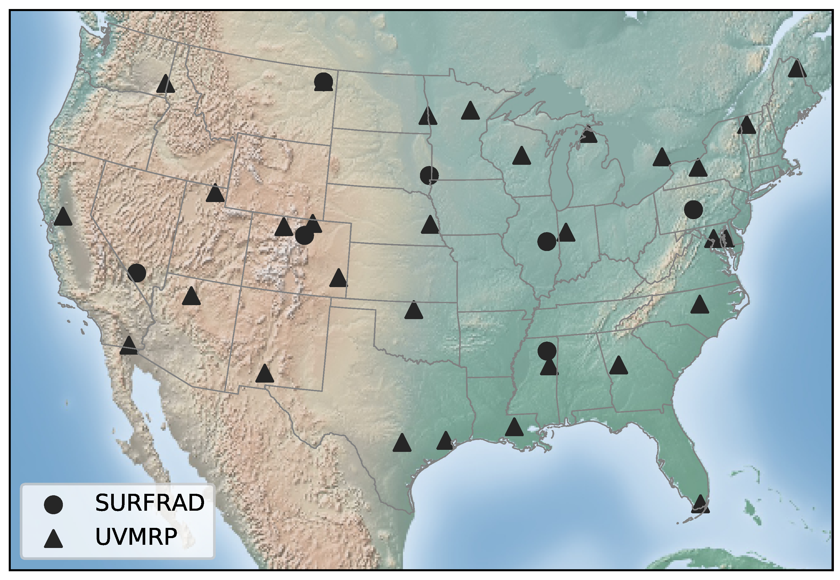
Figure 1. Study site distribution map. The triangular markers denote the site locations of the UV-B Monitoring and Research Program (UVMRP) network. The circle markers denote site locations of Surface Radiation Budget Network (SURFRAD).
Remotesensing 14 00384 g001
Figure 2. The structure of the proposed deep learning (DL)-based erythemal ultraviolet-B (UV-B) retrieval framework.
Remotesensing 14 00384 g002
Figure 3. The structure for the residual layer.
Remotesensing 14 00384 g003
Figure 4. Comparison between measured erythemal UV-B and estimated UV-B on SURFRAD test data: (a) FCNN model; (b) DRFCN model; (c) FCNN+RF model; (d) DRFCN+RF model.
Remotesensing 14 00384 g004
Figure 5. The Taylor diagram that depict R, N S D , and N R M S D for the DRFCN+RF vs. DRFCN, FCNN+RF, and FCNN models on SURFRAD test set. The point labeled groundtruth represents a reference value. The circles represent the models, and the color of each circle represents the n M B E   ( % ) .
Remotesensing 14 00384 g005
Figure 6. Comparison between measured erythemal UV-B and estimated erythemal UV-B on SURFRAD test data: (a) SVR model; (b) RF model; (c) DRFCN+SVR model; (d) DRFCN+RF model.
Remotesensing 14 00384 g006
Figure 7. A line chart of comparison of the R M S E generated by DRFCN+RF vs. the DRFCN+SVR, RF, and SVR models.
Remotesensing 14 00384 g007
Figure 8. Comparison between measured and estimated erythemal UV-B on SURFRAD test data: (a) shows the evaluation results of the entire SURFRAD test set, while (bh) show the results of one station in the SURFRAD test set.
Remotesensing 14 00384 g008
Figure 9. Taylor Diagrams for evaluating DRFCN+RF on SURFRAD test data. The point labeled groundtruth represents the reference value. The color of each circle represents the n M B E ( % ) .
Remotesensing 14 00384 g009
Figure 10. The Taylor diagrams for evaluating DRFCN+RF on SURFRAD-2017 dataset. The point labeled ground truth represents a reference value. The color of each circle represents the n M B E (%).
Remotesensing 14 00384 g010
Figure 11. Performance evaluation of the DRFCN+RF model on the UVMRP dataset by R 2 and n R M S E ( % ) . The n R M S E ( % ) and R 2 are displayed on the left and right axes, respectively.
Remotesensing 14 00384 g011
Figure 12. Taylor diagrams for evaluating DRFCN+RF on UVMRP dataset. The point labeled groundtruth represents the reference value. The color of each circle represents the n M B E   ( % ) .
Remotesensing 14 00384 g012
Table 1. The geographic information of SURFRAD and UVMRP sites used in this paper.
Observation
Network
Station IDLocationLatitude (°N)Longitude (°W)Elevation (m)
SURFRADBONBondville, Illinois40.0588.37213
DRADesert Rock, Nevada36.62116.021007
FPKFort Peck, Montana48.31105.10634
GWNGoodwin Creek, Mississippi34.2589.8798
PSUPenn. State Univ., Pennsylvania40.7277.93376
SXFSioux Falls, South Dakota43.7396.62473
TBLTable Mountain,
Boulder, Colorado
40.12105.241689
UVMRPAK01Fairbanks, Alaska65.12147.43509
AZ01Flagstaff, Arizona36.06112.182073
CA01Davis, California38.53121.7818
CA21Holtville,  California32.81115.45−18
CO01Nunn, Colorado40.81104.761641
CO11Steamboat Springs, 
Colorado
40.46106.743220
CO41Lamar, Colorado38.07102.621131
FL01Homestead, Florida25.3980.680
GA01Griffin, Georgia33.1884.41267
IN01West Lafayette, Indiana40.4786.99216
LA01Baton Rouge, Louisiana30.3691.176
ME11Presque Isle, Maine40.7068.04155
MD01Queenstown,  Maryland38.9276.155
MD11Beltsville, Maryland39.0176.9564
MI01Pellston, Michigan45.5684.68230
MN01Grand Rapids, 
Minnesota
47.1893.53424
MS01Starkville, Mississippi33.4788.7888
MT01Poplar, Montana48.31105.10634
NC01Raleigh, North Carolina35.7378.68120
ND01Fargo, North Dakota46.9096.81275
NE01Mead, Nebraska41.1596.49355
NM01Las Cruces, 
New Mexico
32.62106.741317
NY01Geneva, New York42.8877.03219
OK01Billings, Oklahoma36.6097.49317
ON01Toronto, Ontario43.7879.47210
TX21Seguin, Texas29.5797.98172
TX41Houston, Texas29.7295.3476
UT01Logan, Utah41.67111.891369
VT01Burlington, Vermont44.5372.87390
WA01Pullman, Washington46.76117.19805
WI01Dancy, Wisconsin44.7189.77381
Table 2. Performance evaluation of the deep residual fully connected network plus random forest (DRFCN+RF) model under different parameter combinations. The best combination is marked in red. “TOA” refers to the spectral top-of-atmosphere (TOA) reflectance in the Moderate Resolution Imaging Spectroradiometer (MODIS) bands.
Model Input R 2 MBE
(mW/m 2 )
nMBE
(%)
RMSE
(mW/m 2 )
nRMSE
(%)
TOA0.8733−7.62−7.56%25.0324.84%
TOA + SZA + VZA0.9217−4.01−3.98%19.6819.53%
TOA + SZA + VZA + altitude0.9401−2.79−2.77%17.2117.08%
TOA + SZA + VZA + altitude
+ VAA + SAA
0.9266−4.00−3.97%19.0618.91%
TOA + SZA + VZA + altitude + latitude0.9330−3.18−3.16%18.2118.07%
TOA + SZA + VZA + altitude + ozone0.9649−1.03−1.02%13.113.08%
TOA + SZA + VZA + altitude + ozone + surface reflectance0.98870.190.19%7.487.42%
SZA: solar zenith angle; VZA: view zenith angle; SAA: solar azimuth angle; R2: coefficient of determination; MBE: mean bias error; nMBE: normalized MBE; RMSE: root mean square error; nRMSE: normalized RMSE.
Table 3. Performance evaluation of the DRFCN+RF, DRFCN, fully connected neural network (FCNN), FCNN+RF models by R 2 , n R M S E , coefficient of correlation (R), normalized standard deviation ( N S D ), and normalized centered root-mean-square difference ( N R M S D ). The best model is marked in red.
All stations
Model R 2 n R M S E (mW/m 2 )R N S D N R M S D
FCNN0.916720.14%0.96440.89310.27
DRFCN0.938117.36%0.97030.94370.24
FCNN+RF0.972511.57%0.98650.96090.17
DRFCN+RF0.98877.42%0.99440.98720.11
BON
Model R 2 n R M S E (mW/m 2 )R N S D N R M S D
FCNN0.903421.14%0.95190.95120.31
DRFCN0.919619.29%0.95970.97260.28
FCNN+RF0.969111.96%0.98440.98960.18
DRFCN+RF0.98598.05%0.99300.99030.12
DRA
FCNN0.944113.45%0.98180.91080.20
DRFCN0.968610.90%0.98520.96420.17
FCNN+RF0.97908.25%0.99010.95790.14
DRFCN+RF0.99254.92%0.99630.99320.09
FPK
Model R 2 n R M S E (mW/m 2 )R N S D N R M S D
FCNN0.931218.29%0.96970.89510.26
DRFCN0.949815.63%0.97750.92780.22
FCNN+RF0.958514.21%0.98000.96460.20
DRFCN+RF0.98847.52%0.99430.97800.11
GWN
Model R 2 n R M S E (mW/m 2 )R N S D N R M S D
FCNN0.876922.73%0.95630.82600.32
DRFCN0.899020.59%0.96010.85440.30
FCNN+RF0.961212.76%0.98500.91520.19
DRFCN+RF0.98527.87%0.99310.96170.12
PSU
Model R 2 n R M S E (mW/m 2 )R N S D N R M S D
FCNN0.880423.97%0.94220.89870.34
DRFCN0.894622.49%0.94700.91840.32
FCNN+RF0.966112.75%0.98310.97270.18
DRFCN+RF0.98179.36%0.99090.97970.13
SXF
Model R 2 n R M S E (mW/m 2 )R N S D N R M S D
FCNN0.917022.23%0.96550.89990.27
DRFCN0.941718.62%0.97270.94260.23
FCNN+RF0.965314.37%0.98280.96320.19
DRFCN+RF0.99226.79%0.99610.99170.09
TBL
Model R 2 n R M S E (mW/m 2 )R N S D N R M S D
FCNN0.862323.50%0.94000.85170.35
DRFCN0.900220.00%0.95110.94330.30
FCNN+RF0.971610.66%0.98630.95310.17
DRFCN+RF0.98148.65%0.99060.98490.14
Table 4. Performance evaluation of the support vector regression (SVR), RF, DRFCN+RF, and DRFCN+SVR models by R 2 , n R M S E , R, N S D , and N R M S D . The best model is marked in red.
All stations
Model R 2 n R M S E (mW/m 2 )R N S D N R M S D
SVR0.889023.25%0.94410.90780.33
RF0.918819.88%0.95860.95340.28
DRFCN+SVR0.961813.65%0.98090.96150.19
DRFCN+RF0.98877.42%0.99440.98720.11
BON
Model R 2 n R M S E (mW/m 2 )R N S D N R M S D
SVR0.870624.47%0.93630.95390.36
RF0.881823.39%0.93940.95560.34
DRFCN+SVR0.922918.88%0.96100.98520.28
DRFCN+RF0.98598.05%0.99300.99030.12
DRA
Model R 2 n R M S E (mW/m 2 )R N S D N R M S D
SVR0.910217.05%0.95970.88950.29
RF0.957811.69%0.97870.97590.21
DRFCN+SVR0.97049.79%0.98560.95780.17
DRFCN+RF0.99254.92%0.99630.99320.09
FPK
Model R 2 n R M S E (mW/m 2 )R N S D N R M S D
SVR0.909420.98%0.95410.97170.30
RF0.926718.88%0.96270.95040.27
DRFCN+SVR0.954014.95%0.97710.96370.21
DRFCN+RF0.98847.52%0.99430.97800.11
GWN
Model R 2 n R M S E (mW/m 2 )R N S D N R M S D
SVR0.835926.25%0.92540.80710.40
RF0.880322.41%0.93890.91340.35
DRFCN+SVR0.955813.61%0.98250.91690.20
DRFCN+RF0.98527.87%0.99310.96170.12
PSU
Model R 2 n R M S E (mW/m 2 )R N S D N R M S D
SVR0.869125.07%0.93390.96780.36
RF0.882123.80%0.94050.91640.34
DRFCN+SVR0.958814.05%0.97970.96820.20
DRFCN+RF0.98179.36%0.99090.97970.13
SXF
Model R 2 n R M S E (mW/m 2 )R N S D N R M S D
SVR0.913522.69%0.95580.94730.29
RF0.925521.06%0.96260.99350.27
DRFCN+SVR0.952416.83%0.97640.96480.22
DRFCN+RF0.99226.79%0.99610.99170.09
TBL
Model R 2 nRMSE (mW/m 2 )R N S D N R M S D
SVR0.810127.60%0.90930.86040.42
RF0.864523.31%0.93150.94200.36
DRFCN+SVR0.963812.04%0.98270.94240.19
DRFCN+RF0.98148.65%0.99060.98490.14
Table 5. Performance evaluation of the DRFCN+RF model on the SURFRAD test set (including the results of the seven stations of SURFRAD and their aggregated results).
Stations R 2 MBE (mW/m 2 ) nMBE (%) RMSE (mW/m 2 ) nRSE (%)R NSD NRMSD
BON0.98590.240.27%7.008.05%0.99300.99030.12
DRA0.99250.870.61%6.974.92%0.99630.99320.09
FPK0.9884−0.07−0.08%6.277.52%0.99430.97810.11
GWN0.9852−0.88−0.83%8.097.87%0.99320.96170.12
PSU0.98170.470.55%8.009.36%0.99090.97970.13
SXF0.99220.130.18%5.186.79%0.99610.99170.09
TBL0.98140.250.21%10.258.65%0.99070.98500.14
All station0.98870.190.19%7.487.42%0.99440.98720.11
Table 6. Performance evaluation of the DRFCN+RF model on the SURFRAD-2017 dataset (including the results of the SURFRAD seven stations and their aggregated results).
Stations R 2 MBE (mW/m 2 ) nMBE (%) RMSE (mW/m 2 ) nRSE (%)R NSD NRMSD
BON0.94300.560.64%14.8616.91%0.97120.96800.23
DRA0.94514.533.24%18.1412.95%0.97481.01760.22
FPK0.92963.684.60%16.7520.95%0.96691.00990.25
GWN0.8966−3.39−3.32%20.2519.85%0.93820.89240.31
PSU0.89711.211.33%19.0320.83%0.94730.94450.32
SXF0.9515−1.61−2.19%13.9618.91%0.97580.97500.21
TBL0.92581.091.01%19.2917.94%0.96240.97220.27
All station0.93671.241.27%17.4517.88%0.96860.98700.25
Table 7. Performance evaluation of the DRFCN+RF model on the UVMRP dataset by R 2 , n R M S E , n M B E , R, N S D , and N R M S D .
Site Code R 2 nRMSE nMBE R NSD NRMSD
AK010.810734.19%1.19%0.90090.87510.43
AZ010.870319.72%0.99%0.94200.84360.34
CA010.968711.47%−1.01%0.98450.96700.18
CA210.883218.52%5.90%0.94750.99860.32
CO010.940514.77%1.08%0.97000.97770.24
CO110.779033.08%12.96%0.90190.88040.43
CO410.941214.92%−1.64%0.97060.97980.24
FL010.679826.22%1.19%0.82580.86200.56
GA010.835927.12%2.09%0.91530.93640.40
IN010.868728.67%−0.22%0.93240.95780.36
LA010.853423.56%2.94%0.92560.94260.38
MD110.925518.93%−3.02%0.96470.91010.27
MD010.920619.70%−2.62%0.96070.94370.28
ME110.890623.87%1.02%0.94420.95180.33
MN010.911423.48%−1.27%0.95530.92490.30
MS010.880219.58%-0.00%0.93870.97700.35
MT010.936917.26%−0.72%0.96820.95850.25
NC010.866324.19%−2.14%0.93200.89490.36
ND010.932320.31%−2.59%0.96630.94900.26
NE010.925918.91%−0.57%0.96240.99050.27
NM010.913214.60%3.71%0.96141.03530.28
NY010.873421.19%−1.28%0.93480.95090.36
OK010.919218.27%−2.95%0.96180.93670.27
ON010.898121.64%−0.05%0.94800.92340.32
TX210.782828.98%4.06%0.89150.94430.46
TX410.873819.99%−1.42%0.93540.95830.35
UT010.910919.10%1.73%0.95591.00170.30
VT010.873923.61%0.51%0.93490.94320.35
WA010.929419.97%−0.85%0.96420.97860.27
WI010.905321.98%−2.98%0.95360.92320.30
Publisher’s Note: MDPI stays neutral with regard to jurisdictional claims in published maps and institutional affiliations.