Article

Forest Canopy Height Mapping by Synergizing ICESat-2, Sentinel-1, Sentinel-2 and Topographic Information Based on Machine Learning Methods

1
Centre for Forest Operations and Environment, Northeast Forestry University, Harbin 150040, China
2
College of Surveying and Mapping Engineering, Heilongjiang Institute of Technology, Harbin 150050, China
3
College of Engineering and Technology, Northeast Forestry University, Harbin 150040, China
4
Department of Geographical Sciences University of Maryland, College Park, MD 20742, USA
5
Institute of Economic Management Science, Ministry of Natural Resources (Heilongjiang Provincial Research Institute of Surveying and Mapping), Harbin 150081, China
*
Author to whom correspondence should be addressed.
Remote Sens. 2022, 14(2), 364; https://doi.org/10.3390/rs14020364
Submission received: 22 November 2021 / Revised: 6 January 2022 / Accepted: 9 January 2022 / Published: 13 January 2022
(This article belongs to the Section Forest Remote Sensing)

Abstract

:
Spaceborne LiDAR has been widely used to obtain forest canopy heights over large areas, but it is still a challenge to obtain spatio-continuous forest canopy heights with this technology. In order to make up for this deficiency and take advantage of the complementary for multi-source remote sensing data in forest canopy height mapping, a new method to estimate forest canopy height was proposed by synergizing the spaceborne LiDAR (ICESat-2) data, Synthetic Aperture Radar (SAR) data, multi-spectral images, and topographic data considering forest types. In this study, National Geographical Condition Monitoring (NGCM) data was used to extract the distributions of coniferous forest (CF), broadleaf forest (BF), and mixed forest (MF) in Hua’ nan forest area in Heilongjiang Province, China. Accordingly, the forest canopy height estimation models for whole forest (all forests together without distinguishing types, WF), CF, BF, and MF were established, respectively, by Radom Forest (RF) and Gradient Boosting Decision Tree (GBDT). The accuracy for established models and the forest canopy height obtained based on estimation models were validated consequently. The results showed that the forest canopy height estimation models considering forest types had better performance than the model grouping all types of forest together. Compared with GBDT, RF with optimal variables had better performance in forest canopy height estimation with Pearson’s correlation coefficient (R) and the root-mean-squared error (RMSE) values for CF, BF, and MF of 0.72, 0.59, 0.62, and 3.15, 3.37, 3.26 m, respectively. It has been validated that a synergy of ICESat-2 with other remote sensing data can make a crucial contribution to spatio-continuous forest canopy height mapping, especially for areas covered by different types of forest.

Graphical Abstract

1. Introduction

Forests are major components of terrestrial ecosystems and dominate the dynamics of the terrestrial carbon cycle [1]. As one of significant forest attributes, forest canopy height is an important indicator of biomass allocation, carbon storage, forest productivity, and biodiversity [2,3,4]. Accurate forest canopy height map and its spatio-temporal changes also facilitate forest management and policy-making. Although traditional forest inventories such as field surveys can provide detailed information of forest canopy height with high precision, they are time-consuming, laborious manner, and hinder both rapid investigation and large-scale surveys in difficult sites.
Remote sensing technology is one of the most powerful earth observation approaches. It is rapid and has high precision and large coverage, and has been increasingly used in the extraction of forest canopy height for large areas [5]. Among all remote sensing technologies, LiDAR (light detection and ranging) has significantly contributed to the estimation of forest canopy height in the last two decades, because this technology can directly observe the forest canopy in the vertical direction, and can provide three-dimensional information about forest structure. Numerous studies have used ALS (airborne laser scanning) or spaceborne LiDAR to extract forest canopy height, proving its extensive use and great potential for forest canopy height mapping [6,7].
ALS can usually provide forest canopy height with a high precision, but the small spatial coverage of ALS usually makes it difficult to apply in very large forest areas, and the high cost is also an influencing factor that should be considered. The emergence of spaceborne LiDAR can fairly solve the above problems, and its short revisit cycle and large coverage make it possible to obtain regional even global LiDAR data in a shorter time. Among all spaceborne LiDAR satellites, the ICESat-2 (the Ice, Cloud, and Land Elevation Satellite-2) launched by NASA (National Aeronautics and Space Administration) in 2018 has received extensive attention and became more and more popular in forest canopy height mapping. A photon-counting laser altimeter system was employed by this mission to measure the elevation of ice sheets and vegetation height [8,9]. ICESat-2 provides 21 data products ranging from ATL00 to ATL 21 (no ATL05), of which the ATL08 product can offer various scales of canopy coverage along its orbit, including canopy coverage, apparent reflectance, surface slope and roughness, and canopy height. The potential for the ATL08 product to retrieve forest canopy height in a vegetated region has been validated by the comparison with airborne LiDAR data in Finland [10]. However, the ATL08 product can only provide the along-track forest canopy height in 100 × 14 m segments, so it is impossible for this product to directly obtain spatio-continuous forest canopy height for a large area [11].
A common approach employed to solve the above problems is coupling spatio-continuous optical data with LiDAR-derived metrics to map forest canopy height [12,13]. The Sentinel-2 satellite launched by ESA (European Space Agency) in 2015 has become a popular choice because they are able to provide global optical data with a short revisit period, further improving the monitor of forest system dynamics and functioning on a global scale. In recent years, the data of Sentinel-2 satellite has been used by some studies to extract forest canopy height, and achieved reasonable results. Lang et al. [14] used the airborne LiDAR and Sentinel-2 to map vegetation height in the country-level successfully, validating the importance of multi-spectral metrics and texture metrics extracted from Sentinel-2. Jiang et al. [15] conducted a study by synergizing ICESat-2 with Sentinel-2 to extract forest canopy height in Northern China based on different modelling algorithms, and the best result was found to correspond to the “Stacking Method” proposed in that study.
SAR (Synthetic Aperture Radar) is an active earth observation system, which can observe the earth all day without being affected by the weather. Therefore, the disadvantage that the acquisition of optical data is easy to be affected by climate conditions can be made up. Meanwhile, owing to the certain surface penetration ability of this technology, forest canopy can be penetrated by its signal and more information relevant to structure and density can be obtained. Among all satellites equipped with SAR sensor, the Sentinel-1 satellite has been widely used to estimate forest canopy height. In India, Nandy et al. [16] conducted the first attempt to use ICESat-2 and Sentinel-1 to estimate forest canopy height and the forest canopy height map of the study area was obtained. In that study, the important role of backscatters (VH and VV) provided by the C-band SAR carried on Sentinel-1 satellite in mapping forest canopy height was validated, and the above fact can be attributed to that the upper parts of forest canopy can be penetrated by SAR and its signal can even interact with small branches and leaves under crowns. Li et al. [12] coupled ICESat-2 data with Sentinel-1 SAR, Sentinel-2 images and Landsat-8 images to predict forest canopy height in Northeast China based on two machine learning algorithms, and the minimum of R value between the predicted and validation results is 0.68. Liu et al. used only Sentinel-1 SAR data and Sentinel-2 optical images to extract forest stand mean height at 10 m resolution in Northeast China. In that study, different variables extracted from multi-source remote sensing data were used to predict forest stand mean height based on an empirical model, and the best determination coefficient ( R 2 ) and RMSE were 0.53 and 2.92 m, respectively [17].
Machine learning methods have many advantages including lower computational complexity, less need for parameter tuning, stronger capability in classification and regression, and higher performance in integrating multi-source data [18]. Compared with traditional parametric classifiers, machine learning methods are more robust and with higher classification accuracy [19]. In recent years, more and more machine learning methods have been widely used in the fusion of multi-source remote sensing data. In this study, two machine learning algorithms, RF and GBDT, were used to establish height estimation models for different types of forest. Random Forest, based on bagging and random feature selection, is a popular machine learning algorithm and is known to provide high accuracy [20]. As an important mathematical modeling algorithm, RF has been widely used in establishing models between forest attributes and variables extracted from multi-source data [21,22,23]. GBDT is a representative boosting algorithm, which is an iterative decision tree algorithm, and the results of all trees are aggregated as the final result with high precision [24,25]. The GBDT model has been widely used to assess landslide susceptibility and retrieve soil properties [26,27]. In order to verify the accuracy of models constructed for different types of forest and compare the performance of these two algorithms in forest canopy height estimation, both the RF and GBDT were used to construct the height estimation models in this study.
In recent years, more and more studies were devoted to coupling ICESat-2 data with other remote sensing data to obtain forest canopy height in a large area [12,15,16,17]. However, both the topography condition and the forest types information highly related to the forest canopy height were neglected in those studies. Therefore, a machine-learning-based method synergizing the ATL08 product provided by ICESat-2, Sentinel-1 SAR data, Sentinel-2 optical images, and topographic data to obtain spatio-continuous forest canopy height was proposed. In this method, different estimation models were established and fed according to forest types, and the importance of variables corresponding to different forest types was analyzed. To our knowledge, there have been few prior studies using the above remote sensing data to establish models for estimating forest canopy height and analyzing the importance of variables corresponding to different forest types. The specific objectives of this study are as follows:
  • Evaluate the accuracy for height metric (RH95) provided by ATL08 product by comparing with the height metrics derived from ALS data, and determine the best spatial resolution for these two kinds of height metrics in study area;
  • Establish canopy height estimation models for different forest types using multi-source remote sensing data based on machine learning algorithms (RF and GBDT) at the spatial resolution determined in Step (1). Evaluate the accuracy of the estimation models and compare the accuracy of established model for different forest types;
  • Obtain forest canopy height map for study area based on the estimation models for different forest types established in Step (2), and conduct accuracy assessment for the forest canopy height map by comparing with existing forest canopy height map;
  • Obtain optimal variables for different forest types based on machine learning algorithms. Compare the optimal variables corresponding to different forest types and analyze the importance of variables for different forest types.

2. Materials and Methods

2.1. Study Area

Hua’ nan forest area is located in the northeast of Heilongjiang Province, which is a branch belonging to Wanda Mountains, and it is one of the most important forest regions and timber-producing bases for Heilongjiang Province. Forest types in the study area are mainly CF, BF, and MF, with a forest cover rate of ~35.1%. There are various tree species in Hua’nan forest area, mainly including Korean pine, Manchurian ash, fir, oak, and birch. In addition to forests, the land cover of the study area is mainly crop (maize and soybean). The study area has a continental monsoon climate, and the average annual temperature is 3.6 °C. The average annual precipitation is 523.4 mm, in which ~83% of precipitation is concentrated between May and September [28]. In order to verify the potential of the proposed method to obtain spatial-continuous forest canopy height, study area should be selected as large as possible, but the coverage of data used to establish models must also be taken into account. In view of the above two aspects, two study areas were selected as shown in Figure 1. Area 1 covers ~3.12 × 10 3   km 2 , where both ALS data and ICESat-2 data are available, and the coverage of Area 2 is ~6.62 × 10 3   km 2 .
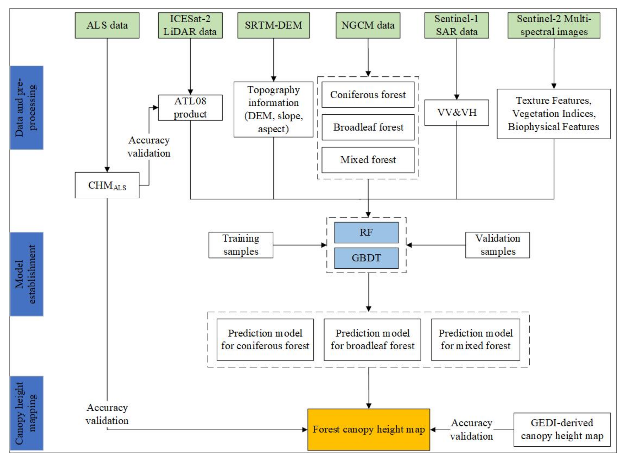
Three steps were included in this study. The first step was data acquisition and preprocessing, mainly including the acquisition and pre-processing for multi-source data used for establishing model. The second step was model establishment, and the main work was establishing canopy height prediction models by machine learning algorithms. Finally, the canopy height for the study area was obtained. The flowchart of the proposed method is shown in Figure 2.

2.2. Data Collection and Preprocessing

The ATL08 product provided by ICESat-2, SAR data provided by Sentinel-1, optical images provided by Sentinel-2, topographic information extracted from SRTM-DEM, NGCM data, and ALS data were used in this study.

2.2.1. ICESat-2 Data

The ICESat-2 was launched in 2018 and this satellite was originally designed to provide continuous observation of sea ice thickness, ice sheet height, and global vegetation height. At the same time, by collecting measurement data over temperate regions, the ICESat-2 satellite can contribute to the production of global carbon inventory [8]. Despite the lack of a formal requirement, the ICESat-2 project office and science team are dedicated to providing height data of terrestrial ecosystems that are useful to the science community. The sensor onboard ICESat-2 is a photon-counting LiDAR (Advanced Topographic Laser Altimeter System, ATLAS), whose repetition rate was much higher than that of other LiDAR detectors, enabling detection of individual photons. The laser of ATLAS is split into six beams (three pairs) that represent the surface. According to the amount of energy carried by the laser, each pair contains a strong beam and a weak beam with the energy ratio of 4:1, indicating that the strong beam will detect four times the number of photons than the weak beam on average [29]. ATL03 from the ICESat-2 mission is a geolocated photon cloud product that serves as the input data for other higher-level data products [30]. Using the DARGANN (Differential, Regressive, and Gaussian Adaptive Nearest Neighbor) algorithm, solar background noises in ATL03 are removed and signal photons are selected [31]. Then, the signal photons are filtered and classified into three types: top of canopy photons, canopy photons, and ground photons. The ATL08 product is produced based on labelled photons over the vegetated surfaces that are recorded by the ICESat-2 sensor within a 100 × 14 m segment [32]. The ATL08 product not only reports information of forest canopy height, some height metrics related to vegetation structure also can be obtained, as shown in Table 1. In this study, the ATL08 RH95 metric was selected as the dependent variable for the estimation model construction according to the previous literature [10].
In this study, ATL08 segments required in 2019 and 2020 were downloaded from NSIDC (National Snow & Ice Data Center), and the strong beam was selected according to the conclusion in [10]. Segments with uncertain estimated heights (the standard deviation of the top of canopy height photons) greater than the average uncertain height were removed according to the uncertain height attribute provided by the ATL08 product. With the help of NGCM data, the forest/non-forest map can be obtained intuitively, and segments within the forest were selected.

2.2.2. Sentinel-1 SAR Data

The Sentinel-1 mission is comprised of two polar-orbiting satellites (1A, 1B) with a 6–12 days revisit period, performing C-band SAR imaging day and night. Due to the penetration ability of SAR, this system is independent of weather and sun illumination and can provide the all-weather mapping capability [12]. Meanwhile, both single- (HH or VV) and dual-polarization (HH + HV or VV + VH) (H: horizontal; V: vertical) operations are supported by this technology. The backscatters including VV and VH are more sensitive to surface scattering and volume scattering [12]. In this study, the backscattering coefficients VV and VH of Sentinel-1 were obtained from the “Sentinel-1 SAR GRD” dataset provided by Google Earth Engine (GEE). In this study, 42 Sentinel-1 images (10 m resolution) were used, and a median composition was applied to each band of Sentinel-1 images based on all high-quality data obtained from the 2020 growing season (June–September).

2.2.3. Sentinel-2 Multi-Spectral Images

Sentinel-2 (twin satellites Sentinel-2A and Sentinel-2B), is a wide-swath, high-resolution, and multi-spectral imaging mission. This mission supports the monitoring of water, soil, and vegetation. The Sentinel-2 satellite provides multi-spectral data with multiple spatial resolutions and can obtain surface feature information on different bands [12]. Meanwhile, the red-edge bands carried by MSI sensor are more sensitive to vegetation growth, so it can provide more accurate information on land changes and vegetation growth [17]. Our study selected the 10 m bands (blue: 490 nm, green: 560 nm, red: 665 nm, and NIR: 842 nm), and 20 m bands (swir1, swir2, and red-edge bands). Because many features used in modelling are related to leaves, Sentinel-2 images not affected by clouds were selected during the leaf-on period (June–September). In this study, 186 Sentinel-2 images were used, and a median composition was applied to each band of Sentinel-2 images based on all high-quality data from June to September in 2020. The Level-2A product was obtained from the Copernicus Scientific Data Hub (CSDB) and the SNAP (Version: 8.0) and Google Earth Engine (GEE) were used for cloud-detection and resampling. Then, biophysical variables, vegetation indices, and texture features were obtained.

2.2.4. Topographic Information

The Shuttle Radar Topographic Mission Digital Elevation Model (SRTM-DEM) dataset was used in this study. The spatial resolution of this product is 30 m and it can provide consistent and high-quality topographic variables including elevation, slope, and aspect, which are closely related to the distribution and growth of vegetation, and will affect the height of vegetation indirectly [33,34]. In this study, the “NASA SRTM Digital Elevation” dataset covering the study area was called and processed by GEE, and then slope, aspect, and elevation were obtained.
Finally, 23 variables were selected to establish a height estimation model, which belonged to the categories “Biophysical Features”, “Vegetation Indices”, “Texture Features”, “VV&VH”, and “Topographic Information”. The variables and their information corresponding to each forest type are shown in Table 2.

2.2.5. NGCM Data

The NGCM (National Geographical Condition Monitoring Project) was launched in 2013 to dynamically monitor Chinese territory [35]. The project was completed through the cooperation of different departments among governments at all levels, representing the authoritative information of China’s geographical conditions. The categories of land surface were divided into three categories, and 12 first-level categories, 58 second-level categories, and 135 third-level categories were all included in the NGCM product [36]. In order to ensure the accuracy of the NGCM product, high-resolution remote sensing data and field data were used to conduct the accuracy assessment [37]. In addition, the quality control of NGCM product was based on “two-level inspection, first-level acceptance, process sampling inspection, and post-test review” [38,39]. The NGCM data covering the study area collected in 2016 was selected in this study. With the help of this data, forest types (CF, BF, and MF) in the study area could be identified.

2.2.6. ALS Data

As shown in Figure 1, the coverage of ALS data is about 193 km 2 , and all three forest types are included. High-precision ALS data were obtained in June 2019 by the SZT-R250 measurement system. This system was developed by an independent Chinese company and it integrates a high-precision laser scanner, a global navigation satellite system, an inertial measurement unit (IMU), a time-synchronization module, and a control module. The LiDAR onboard the SZT-R250 system is a MiniVUX-1UAV whose laser level, emission frequency, and ranging accuracy are “CLASS1”, 100 kHz, and 0.015 m, respectively. With the help of GNSS and IMU, various positioning modes are combined and point cloud data can be obtained in real time, and the average point density is ~64.5 pts / m 2 . After preprocessing the ALS data using LiDAR360 software (Trial Version) provided by Beijing Green Valley, forest canopy height was obtained as the height of the canopy photons minus the corresponding ground elevation. The gridded forest canopy height was set to be the mean value of forest canopy heights in every grid.
All data, including ATL08 data, the generated variables extracted from Sentinel-1 SAR data, Sentinel-2 images, SRTM-DEM, and ALS data were projected to the Universal Transverse Mercator (UTM) Zone 52 N projection based on the WGS-84 ellipsoid. All metrics were composited and resampled to the 250 m resolution according to the result in Section 3.1.

2.3. Forest Canopy Height Prediction

In this study, two machine learning algorithms, RF and GBDT, were used to link the height metric provided by ICESat-2 and variables derived from multi-source remote sensing data.

2.3.1. Random Forest

The RF algorithm is based on the decision tree, which is combined by many ensemble regressions or classification trees [40]. The decision tree uses a bagging or bootstrap algorithm to build a large number of different training subsets [41,42]. The ensemble classifier can be expressed as Equation (1):
h x , θ k ,   k = 1 ,   2 ,   ,
where x is the input sample vector, k is the number of decision trees, and θ k is the parameter vector for the k t h decision tree, which is independent and identically-distributed random vector. For the non-training samples, a classification result will be provided by each decision tree. Then, the decision tree will “vote” for this result, and the final class is determined by the largest number of votes [43].
Owing to the enhancement of the ability for noise removal by randomization, this algorithm is not susceptible to over-fitting and can handle thousands of input variables without variable deletion. Meanwhile, variable importance can be obtained by the permutation method. This method will create a tree and then calculate accuracy using out-of-bag observations (OOB) [44]. Then, the permutation process will run in an iterative manner for all input variables and the variable importance for final permutation is calculated from the average value of all importance values. The optimal variable set corresponding to each model can also be obtained by the following steps below. First, all candidate variables are used to establish estimation model and then the OOB value and importance score are calculated for each. Second, the variable with the lowest score is removed and the remaining variables are used to reestablish the model. These steps are repeated to calculate the OOB value and variable importance for each run. Finally, the optimal model and estimation variables are determined by the minimum OOB value.

2.3.2. Gradient Boosting Decision Tree

GBDT is the combination of “Gradient Boosting” and “Decision Tree”. The idea of Gradient Boosting is that for a complex task, it is better to synthesize the judgment of multiple experts than any one of them, so this algorithm can be regarded as an additive model composed of M trees, which can be expressed as Equation (2):
F x ,   w = m = 0 M α m h m x ,   w m = m = 0 M f m x ,   w m
where x is the input sample, w is the model parameter, h is the regression tree for classification, and α is the weight of each tree.
The Decision Tree algorithm divides an unknown data set by learning the rules through decisive features. This algorithm needs less engineering for features and can automatically combine multiple features. The Gradient Boosting and Decision Tree algorithm combination can solve the over-fitting problem when utilizing the Decision Tree algorithm alone. The base learner of a GBDT algorithm in classification and regression is a Classification and Regression Trees (CART), and the output of each iteration is different. The output to be fitted in this round is the difference between the predicted value and actual value of the previous model (model residual). The GBDT algorithm offers many loss functions that can deal with classification and regression problems. The advantages of GBDT algorithm include the ability to process all kinds of data, high accuracy of estimation, and robust loss functions to deal with outliers.
In this study, height estimation models for the whole forest, coniferous forest, broadleaf forest, and mixed forest were established using RF and GBDT, and these two algorithms were called by the “scikit-learn” package embedded in Python (Version: 3.8). The two RF parameters were set as follows: the number of decision trees (n_estimators) was set to 300, the maximum depth of a tree (max_depth) was set to 50, and other parameters were set as default. For GBDT, the parameter n_estimators, max_depth, subsample, learning rate, loss was selected as 200, 7, 0.9, 0.1, and “ls”. It should be noted that the selection of training samples and validation samples for GBDT algorithm was identical to the RF algorithm.

3. Results

3.1. Accuracy of ATL08 Product and Sample Selection

The forest canopy height provided by the RH95 metric of ATL08 product ranged from 2.09 to 36.65 m with an average value of 16.07 m, and the potential for the ATL08 product to represent forest canopy height should be validated. In order to verify the accuracy of RH95 metric in the study area, height metrics at different pixel sizes were calculated from the normalized height of the ALS point clouds with the geographic locations of the ICESat-2 footprints as the centroids [12]. The area covered by ALS data included all three forest types and a total of 145 points were obtained. Five height metrics, including mean height (h_mean), median height (h_median), 90th and 95th percentile height ( h 90 and h 95 ), and maximum height ( h m a x ), were derived from the airborne point cloud data after reprocessing [45].
According to spatial resolution of common satellite images, the pixel size was selected as 10, 30, and 250 m to extrapolate the canopy height by ALS data. Finally, two accuracy indicators (R and RMSE) were calculated for the ATL08 and ALS data. Table 3 shows the values of R and RMSE for the RH95 and derived heights from ALS data for different spatial scales. It could be seen that for 10, 30, and 250 m resolutions, the value of R was 0.23–0.71, 0.54–0.73, and 0.68–0.80, respectively, and the corresponding value ranges of RMSE were 2.69–3.29 m, 2.59–2.98 m, and 1.98–2.45 m. There were good consistencies between the height metrics retrieved from ALS data and RH95. When the spatial resolution is 250 m, the best result was obtained and the corresponding R-value and RMSE-value were 0.80 and 1.98 m. Correlations were much lower at 10 m and 30 m resolutions and the largest differences were found between h m e d i a n and RH95 when the resolution was 10 m, with the R-value and RMSE-value of 0.23 and 3.29 m. A similar result was also obtained in [46], and may be attributed to the similar geographical condition, vegetation, and climate. For the case of 250 m, the statistical significance of the correlation was also calculated, and a p-value less than 0.05 was obtained. A further calculation found that the RH95 tended to underestimate forest canopy height with a mean value of 1.53 m compared to the h 90 at the 250 m resolution.
Based on the above results, all data used in this study was resampled to 250 × 250 m 2 grids, and the grids including ATL08 coordinate would be selected as effective samples. The calculation of height metric for effective samples includes two cases: (1) If there is only one ATL08 coordinate in the grid, the RH95 metric of this segment will be regarded as the height of this sample; (2) If there is more than one ATL08 coordinate, the average value of RH95 of all segments within the grid will be regarded as the height of this sample. Finally, a total of 2647 samples were selected, and the number of samples corresponding to each special forest type is shown in Table 4. All selected samples for each forest type were divided into training subset and testing subset randomly with a ratio of 8:2.

3.2. Forest Canopy Heights Prediction by RF and GBDT

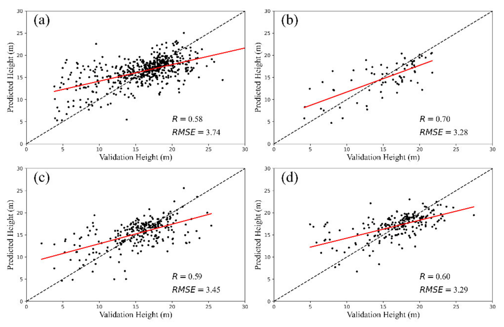
In this study, both RF and GEDT were used to estimate forest canopy height in Area 1. The optimal variables corresponding to the WF, CF, BF, and MF were obtained based on the RF algorithm, and the results are described in Section 3.4. Then, four prediction models for the WF, CF, BF, and MF were established based on the optimal variables. To further demonstrate the performance of the established models for canopy height prediction, values of R and RMSE were calculated for the predicted heights and the validation heights in Area 1. The results are shown in Figure 3 and statistical significances for all correlations are less than 0.05 (p < 0.05).
In Figure 3, R-value ranged from 0.59 to 0.72 and RMSE-value ranged from 3.15 to 3.68 m, indicating the consistency between the predicted and validation heights. Among all results obtained in this study, the prediction model for coniferous forest had the best performance, with R-value and RMSE-value of 0.72 and 3.15 m (Figure 3b). There was overestimation when tree height was less than 15 m. The average value of difference between the predicted results and validation results was calculated, showing an underestimation of ~34.4 cm. Next, the model was established for mixed forest with R-value of 0.62 and RMSE-value of 3.26 m (Figure 3d). When tree height was less than 17.5 m, there was clear overestimation, and underestimation occurred if the height was greater than 17.5 m. The average value of difference between the predicted and validation results was also calculated, and an overestimation of ~48.0 cm was obtained. R-value and RMSE-value for the model corresponding to broadleaf forest were 0.59 and 3.37 m, respectively (Figure 3c). Similarly, the height threshold to distinguish overestimation and underestimation was 16 m and the average value for overestimation was ~3.9 cm. The performance of model for the whole forest was the poorest, whose R-value is 0.59 and RMSE-value is 3.68 m (Figure 3a). It is worth noting that models for whole forest and broadleaf forest had similar performance and both of them were inferior to the results for coniferous and mixed forest.
The GBDT algorithm was also used to establish height prediction models for different forest types and the R and RMSE for the model corresponding to whole forest, coniferous forest, broadleaf forest, and mixed forest were also calculated. Results for predicted and validation canopy heights are shown in Figure 4 and statistical significances for all correlations are less than 0.05 (p < 0.05).
In Figure 4, the prediction model for coniferous forest performed better than the other three prediction models, with R-value of 0.70 and RMSE-value of 3.28 m (Figure 4b). An underestimation of forest canopy height for coniferous forest was detected when tree height was less than 14.0 m. Among all prediction models established by GBDT, the performance of model for mixed forest ranked second, with R-value and RMSE-value of 0.60 and 3.29 m, respectively, and the threshold to discriminate underestimation and overestimation was ~17 m (Figure 4d), meaning that there was underestimation when tree height was less than 17 m. R-value and RMSE-value for the model corresponding to broadleaf forest were 0.59 and 3.45 m, respectively (Figure 4c). Consistent with the case of RF, the poorest result corresponded to the model established for broadleaf forest, where R-value and RMSE-value were 0.59 and 3.45 m, and the height threshold to distinguish underestimation and overestimation was ~15.5 m.
The results for coniferous forest, broadleaf forest, and mixed forest based on these two algorithms all performed better than the model for whole forest, illustrating that the canopy height prediction model established considering forest types had greater potential for forest canopy height estimation than the model established for simply grouping all types of forest together. Meanwhile, the relationship of accuracy for models established by RF and GBDT is consistent, that is, prediction model for coniferous forest has the highest accuracy, model for mixed forest takes the second place, and the accuracy of model for broadleaf forest is the lowest. It can also be found that the GBDT algorithm was not as good as the RF algorithm for all forest types, so RF was selected to predict forest canopy height covering the study area in this study.
Two methods were used to further verify the potential of the prediction models based on RF to obtain spatio-continuous forest canopy height. Firstly, three sub-regions only covered by coniferous forest, broadleaf forest, and mixed forest were selected in Area 1 to validate the ability of the established model in canopy height mapping for single forest type. With the help of NGCM data and Google images, A, B, and C representing coniferous forest, broadleaf forest, and mixed forest were selected and the number of samples locating within coniferous forest, broadleaf forest, and mixed forest were 76, 325, and 340 (Figure 5).
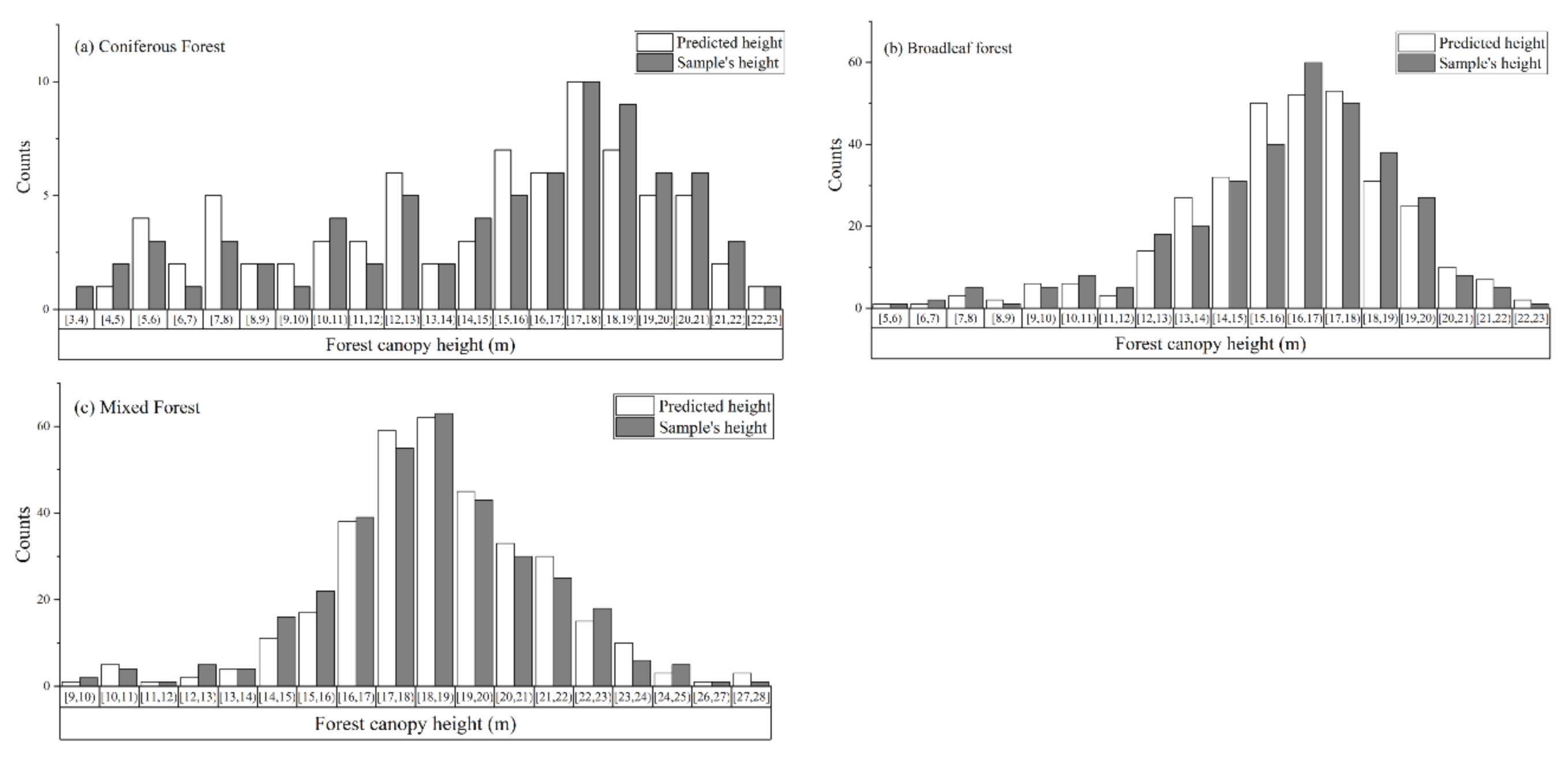
A comparison for predicted forest canopy heights by RF and RH95 metric of samples in three sub-regions was conducted, and the histograms for sample’s heights and predicted heights were obtained and shown in Figure 6, where (a), (b), and (c) represent results for coniferous, broadleaf and mixed forest, respectively.
The results in Figure 6 show satisfying consistency between the predicted forest canopy heights and sample’s forest canopy heights for all forest types. In order to verify the performance of the proposed method intuitively, the minimum difference, maximum difference, and average difference between predicted heights and sample’s heights were calculated. It can be found that the model corresponding to coniferous forest has the best performance, and the minimum and maximum differences between predicted results and validation results are 0.01 and 9.23 m, respectively. The accuracy of the model corresponding to mixed forest is the second, and the minimum and maximum difference between predicted heights and validation heights are 0.01 and 8.92 m respectively. The worst performance belongs to broad-leaf forest, whose minimum and maximum difference between predicted heights and validation heights are 0.29 and 11.37 m, respectively. Meanwhile, the average values of difference between predicted heights and sample’s heights are also calculated and the values corresponding to CF, BF, and MF are 1.80, 2.79, and 1.85 m, respectively, proving that the model for coniferous forest has the best performance in estimating forest canopy height.
In addition, another study area outside the ALS data coverage was used to verify the performance of the models for predicting forest canopy height in a large geographical extent. To achieve the above purpose, the selection of study area should consider the availability of data and expand its area as much as possible. Finally, Area 2 (Figure 1) was selected and the number of samples falling in coniferous forest, broadleaf forest, and mixed forest is shown in Table 5. Forest canopy height in Area 2 was obtained by RF and optimal variables for CF, BF, and MF. Then, the R and RMSE of height metric for samples and predicted results were also calculated. As shown in Table 5, the R-value for CF, BF, and MF are 0.67, 0.50, and 0.61 respectively, and corresponding RMSE-value are 3.16, 3.34, and 3.31 m, indicating that the prediction models corresponding to coniferous forest, broadleaf forest and mixed forest have good performance. The relationship of accuracy between different forest is consistent with the result in Area 1, which can confirm the accuracy and reliability of the canopy height prediction models established in this study.

3.3. Forest Canopy Height Mapping

The forest canopy height for each 250 × 250 m grid in Area 1 was obtained by established prediction models based on RF, and then a forest canopy height map for Area 1 was obtained (Figure 7a). As shown in Figure 7b, the range of predicted canopy heights for CF, BF, and MF are a–b m, a–b m, and a–b m, respectively.
In this study, the accuracy of the forest canopy height map for Area 1 was validated by cross-comparison and spatial analysis. Firstly, a cross-comparison process was conducted between predicted canopy heights and ALS results. Within ALS data coverage, the h 90 metric of ALS and predicted heights by RF were compared for each 250 × 250 m grid and the scatter plot is shown in Figure 8. The Pearson’s correlation coefficient (R) between the predicted canopy height and metric of ALS is 0.58, indicating good correlation between these two kinds of canopy height.
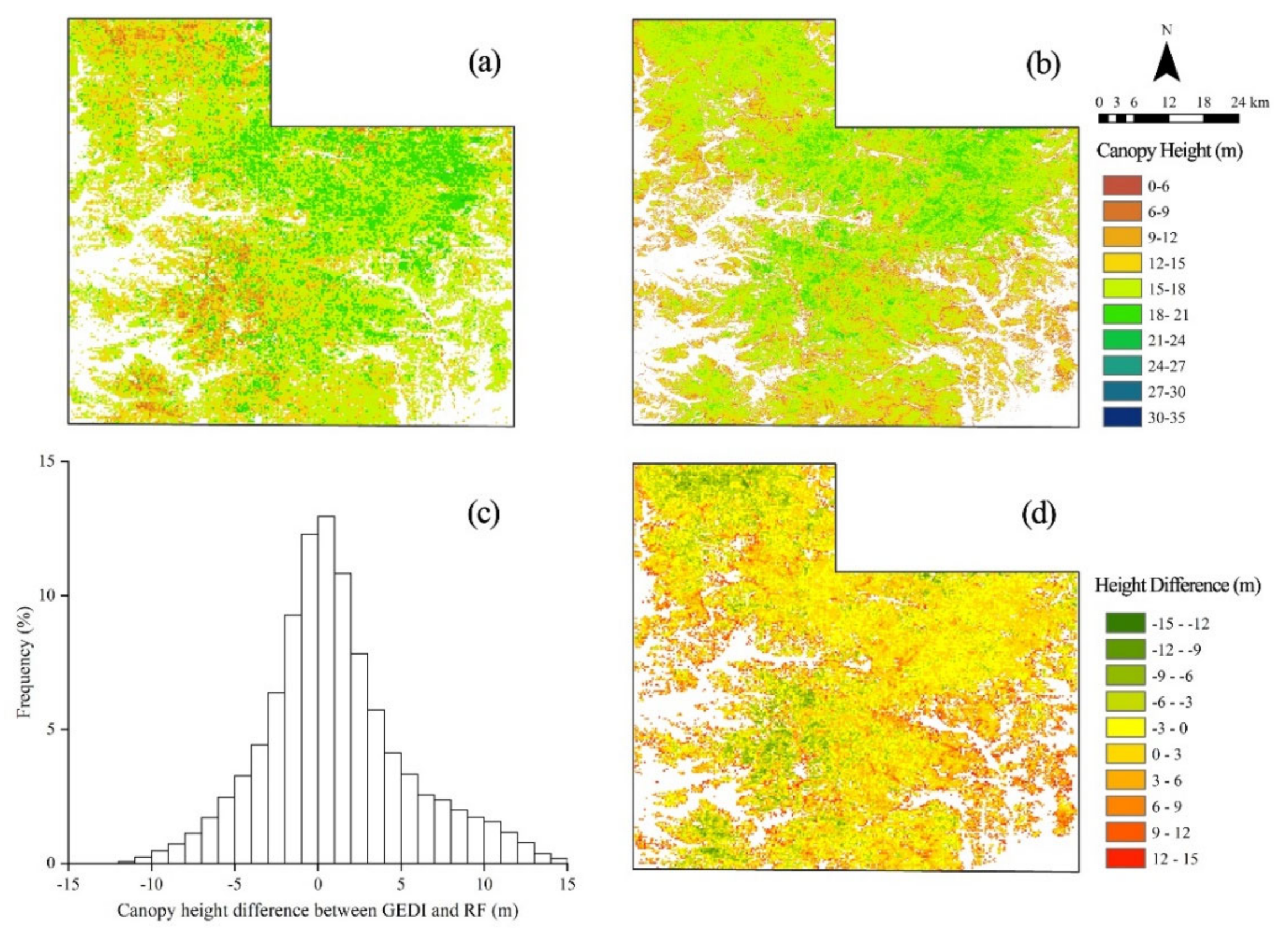
GEDI (Global Ecosystem Dynamics Investigation) is a new spaceborne LiDAR instrument operating onboard the International Space Station (ISS) and has been collecting data between ~51.6° N and ~51.6° S globally by a full waveform LiDAR since April 2019 [47]. By integrating GEDI data with optical metrics derived from Landsat analysis-ready data, a global forest canopy height map with 30 m resolution (GEDI-derived map) for the year 2019 was obtained (https://glad.umd.edu/dataset/gedi/ accessed on 15 September 2021) and the accuracy of the map was assessed quantitatively. In this study, the accuracy of the predicted forest canopy height map for Area 1 was further validated by conducting spatial analysis with GEDI-derived canopy height map. Figure 9a,b represent the predicted canopy height map and GEDI-derived canopy height map in 2019. By visual interpretation, it can be found that the spatial distributions of forest canopy height for these two maps show a similar pattern. For predicted forest canopy height map, the number of grids corresponding to canopy height between 18–24 m is the largest, and for GEDI-derived map, the pixels with canopy height between 15–21 m account for the largest proportion.
Meanwhile, the spatial analysis for predicted forest canopy height map and GEDI-derived map was also carried out based on grids [46]. Firstly, the GEDI-derived map was resampled to 250 × 250 m grid by ArcGIS 10.5 and the corresponding canopy height for each grid was calculated ( G E D I _ h e i g h t ). It can be found that the range of predicted canopy heights and GEDI-derived canopy heights were 5.52–31.13 m and 5–30 m, respectively. Then, a registration process was conducted and canopy height difference for each grid was calculated as Equation (3):
Δ h e i g h t i = p r e _ h e i g h t i G E D I _ h i e g h t i ,   i = 1 , 2 ,   ,
where Δ h e i g h t is canopy height difference for each grid, p r e _ h e i g h t is the canopy height obtained by RF, and i is the number of 250 × 250 m grid in Area 1. Then, the frequency of canopy height difference was calculated. As shown in Figure 9c, the frequency corresponding to a small difference is high, but the frequency corresponding to large difference shows the opposite trend. When the height difference is in 0–1 m, the frequency is the highest, and the frequency corresponding to −1–0 m takes the second place, indicating the difference between the predicted results and GEDI product is mainly in the range of [−1, 1] m. Further statistics show that the number of grids with the difference in the range of [−3, 3] m accounts for ~70% of the total number of pixels, and the average overestimation of predicted canopy height is ~1.05 m (Figure 9d).

3.4. Optimal Variables and Importance Scores

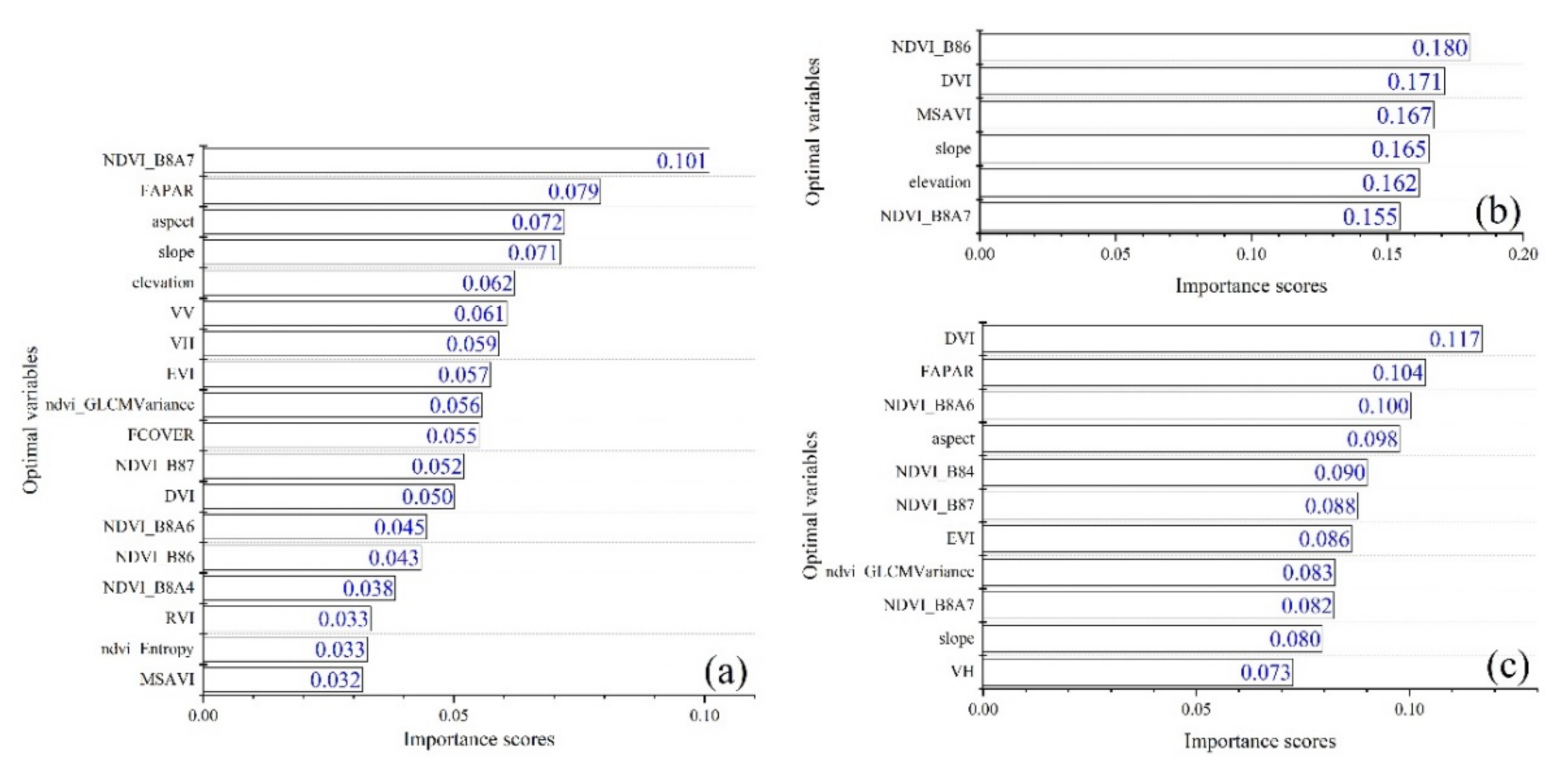
The optimal variables for different estimation models were obtained using the RF algorithm, and the importance score for each variable was evaluated by permutation calculation. The specific variables corresponding to each forest type and their importance scores are shown in Figure 10, where (a), (b), and (c) represent CF, BF, and MF.
The results in Figure 10 show that the most important for coniferous forest, broadleaf forest, and mixed forest models were “NDVI_B8A7”, “NDVI_B86”, and “DVI”. At the same time, there were great differences between variables corresponding to different forest types, which were mainly reflected in the following ways. First, the number of variables in the optimal set for coniferous forest, broadleaf forest, and mixed forest was different, and corresponding values were 18, 6, and 11, respectively. Meanwhile, the specific variables corresponding to each optimal set also varied greatly, and only the “NDVI_B8A7” and “Slope” appeared in all; the rest were not the same. Second, importance score for the same variable differed across optimal sets. For “NDVI_B8A7”, the importance scores for coniferous forest, broadleaf forest, and mixed forest were 0.101, 0.155, and 0.082, and for “Slope”, corresponding scores were 0.071, 0.165, and 0.080. Finally, the distribution of variable scores within the same optimal set were different. For the optimal set corresponding to coniferous forest, the difference between the importance of each variable was distinct, and the situation for mixed forest was quite similar. For broadleaf forest, however, a more uniform distribution of importance was observed and the contribution of each variable to the model was almost identical.
In order to further demonstrate the importance of variables for each optimal set, the sum of the importance for variables belonging to “Biophysical Features”, “Vegetation Indices”, “Texture Features”, “VV&VH”, and “Topographic Information” was calculated and the results are shown in Table 6.

4. Discussion

In this study, a forest canopy height prediction method was proposed based on machine learning algorithms for Hua’ nan forest area in Heilongjiang Province, China, by synergizing ICESat-2 LiDAR data with variables extracted from Sentinel-1 SAR data, Sentinel-2 images, and SRTM-DEM data. The accuracy of prediction models for coniferous forest, broadleaf forest, and mixed forest were validated and the results demonstrated the potential of the proposed method to obtain forest canopy height at a large scale. It is unprecedented to utilize these types of data to map forest canopy height for different types of forest, and the results will be conducive to forest dynamic monitoring and the estimation of other attributes related to forest canopy height.

4.1. Comparison of RF and GBDT for Forest Canopy Height Modelling

In this study, two machine learning algorithms, RF and GBDT, were used to link the forest canopy height provided by ATL08 product and predictor variables extracted from multi-source remote sensing data. Results in Section 3.2 showed that prediction models based on RF algorithm had better performance than models established by GBDT algorithm, and this was true for all three forest types. Both RF and GBDT are tree-based machine learning algorithms and have been widely used in data mining. For the modelling process, several single classifiers are collected by these two algorithms to improve the accuracy. The particular framework and procedure may be responsible for the accuracy difference between RF and GBDT in establishing prediction models [48]. Specially, the RF algorithm can handle complex relationships between predictor variables and data processing capabilities without statistical assumptions, leading the improvement of accuracy by reducing the variance of the model [49]. For the GBDT algorithm, the prediction accuracy is usually improved by reducing the deviation of the model, but the selection of a maximum number of iterations and weight reduction factor may cause over-fitting. He et al. [26] had argued that the RF algorithm could produce more accurate results in landslide susceptibility modelling than GBDT algorithm.
In this study, the advantage of RF algorithm in predicting forest canopy height has been demonstrated, and the prediction models established by RF was suitable for obtaining spatio-continuous forest canopy height for study area. However, the prediction models established by GBDT algorithm provide powerful support for the method proposed in this study, as both machine learning algorithms showed that the method considering forest types had better performance in forest canopy height mapping. Meanwhile, the accuracy of the established models was also verified, because the accuracy corresponding to the two algorithms was consistent, which meant that the prediction model for coniferous forest had the best performance, mixed forest’s model was second, and the model for broadleaf forest had the poorest performance.

4.2. Comparison of Estimation Models for Different Forest Types

In this study, forest canopy height prediction models for whole forest, coniferous forest, broadleaf forest, and mixed forest were established based on machine learning algorithms. Compared with the model for whole forest, accuracy of prediction model for coniferous forest, broadleaf forest, and mixed forest all have been improved, proving the advantage of the method proposed in this study for forest canopy height mapping. This conclusion was comparable with the results from [17], which demonstrated the advantage of distinguishing forest types in predicting forest mean height at stand level in northeast China by utilizing Sentinel-1 and Sentinel-2.
The results in Section 3.2 also showed that the prediction model for coniferous forest had the best performance, and both the results of broadleaf forest and mixed forest were inferior to the result of coniferous forest. The above situation may be attributed to the difference between the accuracy of dependent variables (RH95 metric of ATL08 product) for establishing prediction models. Alexander et al. [7] has confirmed that regardless of the point cloud density used to extract tree height, the accuracy for broadleaf forest was lower than that for coniferous forest. In that study, they explained their conclusion that fewer LiDAR points would reach the ground in the broadleaf forest due to the larger leaf area than coniferous forest, making it difficult to reproduce the true DEM using interpolation method. Mielcarek et al. [50] also argued that the smallest error was obtained for coniferous forest when evaluating different LiDAR-derived canopy height model. In that study, seven tree species were selected to verify the accuracy of different CHM (canopy height model) interpolation methods for predicting tree height by comparing the prediction forest canopy heights with field measured forest canopy heights. As a result, we inferred that the ATL08 product covering coniferous forest has higher accuracy, and the best performance for coniferous forest model can be explained by the higher accuracy of RH95 metric. The necessity to establish prediction models considering different forest types was confirmed once again by conclusions obtained from the above literatures, rather than simply putting all forest types together to estimate forest canopy height, and this situation was true especially for areas covered by different types of forest.

4.3. Comparison of Optimal Variables for Different Forest Types

One of the most important purposes of this study was to determine the optimal variables for different forest types, and results for each estimation model were obtained based on the RF algorithm. The results in Figure 8 show that the optimal variables mainly included vegetation indices, elevation, aspect, slope, VV, and VH. The importance of vegetation indices in forest canopy height estimation has been demonstrated. Pascual et al. [51] conducted the analysis of the relationship between LiDAR-derived forest canopy height and Landsat images, and the results confirmed the important role of vegetation indices when related to the forest canopy height. The elevation, slope, and aspect for estimating forest canopy height were significant geographical and temperature parameters that were closely related to vegetation distribution and growth, and further information on the site properties could be offered by these variables. The offered information on the local variation of forest canopy structure played a crucial role in obtaining meaningful forest attribute maps [33,51]. Meanwhile, the important roles of VV and VH in forest canopy height estimation have also been validated, and our findings were in line with the research of [52], which has reported that VH showed a better correlation with FSMH than VV based on C-band of Radarsat-2 imagery, and a low or even inverse correlation was obtained from VV polarization backscattering.
In Table 6, all kinds of variables from Table 2 were included in the optimal set for coniferous forest and mixed forest, but there were only “Vegetation Indices” and “Topographic Information” variables in the optimal set for broadleaf forest. Table 6 also shows that ‘Vegetation indices’ variables were most important for all forest types, with importance scores of 0.45, 0.67, and 0.57 for coniferous forest, broadleaf forest, and mixed forest, respectively. The second most important category was “Topographic Information”, and the sums of corresponding importance for coniferous forest, broadleaf forest, and mixed forest were 0.21, 0.33, and 0.18.
As a result, 66, 100, and 74% of the variable importance for coniferous forest, broadleaf forest, and mixed forest were explained by the variables provided by “Vegetation Indices” and “Topographic Information”, indicating the important role of these two categories in estimating forest canopy height. Previous studies have shown that there is a strong positive correlation between forest canopy height and vegetation indices, and the potential of vegetation indices in forest canopy height estimation has been demonstrated in [12]. Meanwhile, vegetation species, distribution, and growth are closely related to location, elevation, slope, and aspect; therefore, the topographic variables derived from SRTM-DEM data were particularly important in estimating forest canopy height. The above situation matched results in [17], which showed that slope and aspect were closely related to forest distribution and growth. Therefore, topographic information representing the field environment provides local change information about forest canopy height.
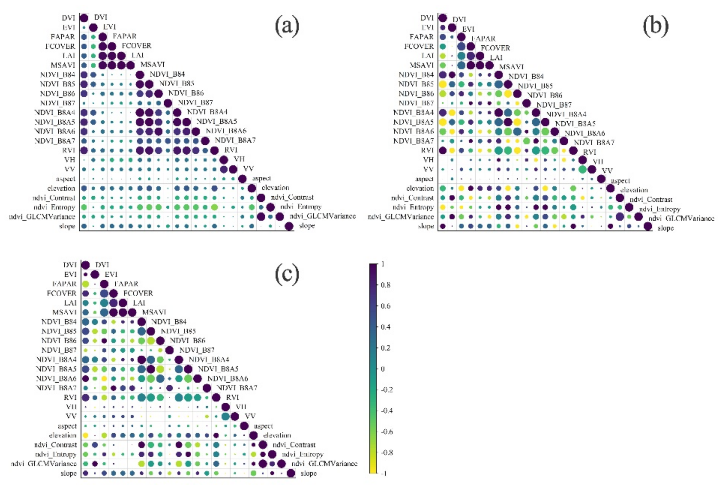
The correlation between variables within each optimal set was further calculated as shown in Figure 11, where (a), (b), and (c) represent coniferous forest, broadleaf forest, and mixed forest, and the color bar indicates the level of correlation. For the three estimation models, significantly positive correlations were observed, such as “NDVI_B8_A4” VS “MSAVI” in the coniferous model, “NDVI_B8_A5” VS “NDVI_B84” in the broadleaf model, and “MSAVI” VS “LAI” in the mixed model. However, there were negative correlations that often appeared in different categories of variables. It is worth noting that variables belonging to the texture feature were negatively correlated with almost all other variables. However, the correlation analysis of variables in each optimal set indicated that although the remaining variables were less important, their roles in model establishment cannot be ignored.
The feasibility of estimating forest canopy height by synergizing multi-source remote sensing data has been verified in this study. Estimation models were established considering forest types, making the predicted results more reliable. Meanwhile, the use of spaceborne data made it possible to obtain forest canopy height for a large area in a short time. The accuracy of height metric of ICEsat-2 product has been verified, providing a basis for using this data in forest canopy height estimation, avoiding the inconvenience in field data collection. However, the acquisition of satellite data is easily affected by weather and climate conditions, which will affect the application of the method proposed in this study. Especially for “Vegetation Indices”, the acquisition of this data will be greatly affected by weather and climate condition and can only be obtained in growing seasons. Meanwhile, the important role of “Topographic Information” has also been analyzed qualitatively because both study areas are located in the northeast plain of China, whose terrain is flat and there is little change between the two study areas. However, for areas with larger coverage, quantitative analysis for topographic information should be conducted to better use the proposed method to obtain forest canopy height. The above situations may affect the application of the model, but the conclusions of this study will have important significance for the selection of variables for constructing canopy height estimation models.

5. Conclusions

In this study, we proposed a new method to estimate forest canopy height by synergizing ICESat-2, Sentinel-1 SAR, Sentinel-2 images, and SRTM-DEM data considering forest types. The accuracy of RH95 metric provided by the ATL08 product of ICESat-2 was validated using airborne LiDAR data, and the highest consistency between ALS data and RH95 metric was detected when the spatial resolution was 250 m. To verify the accuracy, two machine learning methods were used to establish height estimation models for different forest types, and the results showed that the RF algorithm outperformed the GBDT algorithm throughout all forest types, but the relationship of accuracy for different models was consistent. The proposed method obtained more robust results than simply establishing an estimation model without distinguishing forest types, and this situation was true especially for coniferous forest, which had the greatest improvement in accuracy. Meanwhile, the optimal variables for each forest type were obtained based on the RF algorithm, and it is worth noting that variables belonging to “Vegetation indices” and “Topographic information” were in the most important position for all three forest types. As far as we know, no research has used topographic information coupling ICESat-2 data, Sentinel-1 SAR data, and Sentinel-2 multi-spectral images to map forest canopy height in the study area. Further studies should focus on exploring the use of other remote sensing data such as GEDI, Sentinel-3, and GaoFen-7 to estimate forest canopy height for larger areas, aiming to make full use of their complementary advantages and overcome the impact of bad weather on data acquisition.

Author Contributions

Z.X., H.X., and Y.X. conceived and designed the experiments; Z.X. performed the experiments; Z.X. and W.G. analyzed the data; G.C. and S.Y. contributed materials; Z.X., H.X., and Y.X. wrote the paper; Y.X. secured funding for the project; W.G. polished the language of the manuscript. All authors have read and agreed to the published version of the manuscript.

Funding

This research is supported by the National Key R&D Program of China (Grant Number: 2021YFE0117700-6).

Data Availability Statement

Not applicable.

Acknowledgments

We thank the editor and anonymous reviewers for reviewing our paper.

Conflicts of Interest

The authors declare no conflict of interest.

References

  1. Dong, J.; Kaufmann, R.K.; Myneni, R.B.; Tucker, C.J.; Kauppi, P.E.; Liski, J.; Buermann, W.; Alexeyev, V.; Hughes, M.K. Remote sensing estimates of boreal and temperate forest woody biomass: Carbon pools, sources, and sinks. Remote Sens. Environ. 2003, 84, 393–410. [Google Scholar] [CrossRef] [Green Version]
  2. Lefsky, M.A.; Cohen, W.B.; Harding, D.J.; Parker, G.G.; Acker, S.A.; Gower, S.T. Lidar remote sensing of above-ground biomass in three biomes. Glob. Ecol. Biogeogr. 2002, 11, 393–399. [Google Scholar] [CrossRef] [Green Version]
  3. Simard, M.; Pinto, N.; Fisher, J.B.; Baccini, A. Mapping forest height globally with spaceborne lidar. J. Geophys. Res. Biogeosci. 2011, 116. [Google Scholar] [CrossRef] [Green Version]
  4. Zhang, L.; Du, B. Deep learning for remote sensing data: A technical tutorial on the state of the art. IEEE Geosci. Remote Sens. Mag. 2016, 4, 22–40. [Google Scholar] [CrossRef]
  5. Rosenqvist, A.; Milne, A.; Lucas, R.; Imhoff, M.; Dobson, C. A review of remote sensing technology in support of the Kyoto protocol. Environ. Sci. Policy 2003, 6, 441–455. [Google Scholar] [CrossRef]
  6. Wulder, M.A.; White, J.C.; Nelson, R.F.; Næsset, E.; Ørka, H.O.; Coops, N.C.; Hilker, T.; Bater, C.W.; Gobakken, T. Lidar sampling for large-area forest characterization: A review. Remote Sens. Environ. 2012, 121, 196–209. [Google Scholar] [CrossRef] [Green Version]
  7. Alexander, C.; Korstjens, A.H.; Hill, R.A. Influence of micro-topographic and crown characteristics on tree height estimations in tropical forests based on LiDAR canopy height models. Int. J. Appl. Earth Obs. Geoinf. 2018, 65, 105–113. [Google Scholar] [CrossRef]
  8. Markus, T.; Neumann, T.; Martino, A.; Abdalati, W.; Brunt, K.; Csatho, B.; Farrell, S.; Fricker, H.; Gardner, A.; Harding, D. The ice, cloud, and land elevation satellite-2 (ICESat-2): Science requirements, concept, and implementation. Remote Sens. Environ. 2017, 190, 260–273. [Google Scholar] [CrossRef]
  9. Magruder, L.A.; Brunt, K.M. Performance analysis of airborne photon- counting lidar data in preparation for the ICESat-2 mission. IEEE Trans. Geosci. Remote Sens. 2018, 56, 2911–2918. [Google Scholar] [CrossRef]
  10. Neuenschwander, A.L.; Magruder, L.A. Canopy and Terrain Height Retrievals with ICESat-2: A First Look. Remote Sens. 2019, 11, 1721. [Google Scholar] [CrossRef] [Green Version]
  11. Xing, Y.; Huang, J.; Gruen, A.; Qin, L. Assessing the Performance of ICESat-2/ATLAS Multi-Channel Photon Data for Estimating Ground Topographic in Forested Terrain. Remote Sens. 2020, 12, 2084. [Google Scholar] [CrossRef]
  12. Li, W.; Niu, Z.; Shang, R.; Qin, Y.; Wang, L.; Chen, H. High-resolution mapping of forest height using machine learning by coupling ICESat-2 LiDAR with Sentinel-1, Sentinel-2 and Landsat-8 data. Int. J. Appl. Earth Obs. Geoinf. 2020, 92, 102163. [Google Scholar] [CrossRef]
  13. Lin, X.; Xu, M.; Cao, C.; Dang, Y.; Bashir, B.; Xie, B.; Huang, Z. Estimates of Forest height Using a Combination of ICESat-2/ATLAS Data and Stereo-Photogrammetry. Remote Sens. 2020, 12, 3649. [Google Scholar] [CrossRef]
  14. Lang, N.; Schindler, K.; Wegner, J.D. Country-wide high-resolution vegetation height mapping with Sentinel-2. Remote Sens. Environ. 2019, 233, 111347. [Google Scholar] [CrossRef] [Green Version]
  15. Jiang, F.; Zhao, F.; Ma, K.; Li, D.; Sun, H. Mapping the Forest height in Northern China by Synergizing ICESat-2 with Sentinel-2 Using a Stacking Algorithm. Remote Sens. 2021, 13, 1535. [Google Scholar] [CrossRef]
  16. Nandy, S.; Srinet, R.; Padalia, H. Mapping Forest Height and Aboveground Biomass by Integrating ICESat-2, Sentinel-1 and Sentinel-2 Data Using Random Forest Algorithm in Northwest Himalayan Foothills of India. Geophys. Res. Lett. 2021, 14, e2021GL093799. [Google Scholar] [CrossRef]
  17. Liu, Y.; Gong, W.; Xing, Y.; Hu, X.; Gong, J. Estimation of the forest stand mean height and aboveground biomass in Northeast China using SAR Sentinel-1B, multispectral Sentinel-2A, and DEM imagery. ISPRS J. Photogramm. Remote Sens. 2019, 151, 277–289. [Google Scholar] [CrossRef]
  18. Liu, T.; Abd-Elrahman, A.; Morton, J.; Wilhelm, V.L. Comparing fully convolutional networks, random forest, support vector machine, and patch-based deep convolutional neural networks for object-based wetland mapping using images from small unmanned aircraft system. GISci. Remote Sens. 2018, 55, 243–264. [Google Scholar] [CrossRef]
  19. Maxwell, A.E.; Warner, T.A.; Fang, F. Implementation of machine-learning classification in remote sensing: An applied review. Int. J. Remote Sens. 2018, 39, 2784–2817. [Google Scholar] [CrossRef] [Green Version]
  20. Belgiu, M.; Drăgut, L. Random forest in remote sensing: A review of applications and future directions. ISPRS J. Photogramm. Remote Sens. 2016, 114, 24–31. [Google Scholar] [CrossRef]
  21. Ahmed, O.S.; Franklin, S.E.; Wulder, M.A.; White, J.C. Characterizing stand-level forest canopy cover and height using Landsat time series, samples of airborne LiDAR, and the Random Forest algorithm. ISPRS J. Photogramm. Remote Sens. 2015, 101, 89–101. [Google Scholar] [CrossRef]
  22. Lary, D.J.; Alavi, A.H.; Gandomi, A.H.; Walker, A.L. Machine learning in geosciences and remote sensing. Geosci. Front. 2016, 7, 3–10. [Google Scholar] [CrossRef] [Green Version]
  23. Tian, X.; Li, Z.; Su, Z.; Chen, E.; van der Tol, C.; Li, X.; Guo, Y.; Li, L.; Ling, F. Estimating montane forest above-ground biomass in the upper reaches of the Heihe River Basin using Landsat-TM data. Int. J. Remote Sens. 2014, 35, 7339–7362. [Google Scholar] [CrossRef] [Green Version]
  24. Liang, Z.; Wang, C.; Khan, K.U.J. Application and Comparison of Different Ensemble Learning Machines Combining with a Novel Sampling Strategy for Shallow Landslide Susceptibility Mapping. Stoch. Environ. Res. Risk Assess 2021, 35, 1243–1256. [Google Scholar] [CrossRef]
  25. Wang, Y.; Feng, L.; Li, S.; Ren, F.; Du, Q. A Hybrid Model Considering Spatial Heterogeneity for Landslide Susceptibility Mapping in Zhejiang Province, China. CATENA 2020, 188, 104425. [Google Scholar] [CrossRef]
  26. He, Q.; Jiang, Z.; Wang, M.; Liu, K. Landslide and Wildfire Susceptibility Assessment in Southeast Asia Using Ensemble Machine Learning Methods. Remote Sens. 2021, 13, 1572. [Google Scholar] [CrossRef]
  27. Liu, L.; Ji, M.; Buchroithner, M. Combining Partial Least Squares and the Gradient-Boosting Method for Soil Property Retrieval Using Visible Near-Infrared Shortwave Infrared Spectra. Remote Sens. 2017, 9, 1299. [Google Scholar] [CrossRef] [Green Version]
  28. Heilongjiang Meteorological Bureau. Available online: http://http://hl.cma.gov.cn/ (accessed on 10 March 2021).
  29. Neumann, T.; Martino, A.; Markus, T.; Bae, S.; Bock, M.; Brenner, A.; Brunt, K.; Cavanaugh, J.; Fernandes, S.; Hancock, D.; et al. The Ice, Cloud, and Land Elevation Satellite-2 Mission: A global geolocated photon product derived from the Advanced Topographic Laser Al-timeter System. Remote Sens. Environ. 2019, 233, 111325. [Google Scholar] [CrossRef] [PubMed]
  30. Neuenschwander, A.; Pitts, K. The ATL08 land and vegetation product for the ICESat-2 Mission. Remote Sens. Environ. 2019, 221, 247–259. [Google Scholar] [CrossRef]
  31. Neuenschwander, A.L. Ice, Cloud, and Land Elevation Satellite-2 Algorithm Theoretical Basis Document for Land—Vegetation Along-Track Products. Available online: https://icesat-2.gsfc.nasa.gov/sites/default/files/files/ATL08_15June2018.pdf (accessed on 20 May 2021).
  32. Day, F.P.; Monk, C.D. Vegetation patterns on a southern Appalachian watershed. Ecology 1974, 55, 1064–1074. [Google Scholar] [CrossRef] [Green Version]
  33. Ying, W.; Wanxing, Z.; Liqiong, Z.; Jing, W. Analysis of correlation between terrain and forest spatial distribution based on DEM. J. Northeast For. Univ. 2012, 11, 96–98. [Google Scholar]
  34. Zhang, J.; Liu, J.; Zhai, L.; Hou, W. Implementation of Geographical Conditions Monitoring in Beijing-Tianjin-Hebei, China. ISPRS Int. J. Geo-Inf. 2016, 5, 89. [Google Scholar] [CrossRef] [Green Version]
  35. Zhao, Y.; Cai, Y. The application of the national geographic census results in quality inspection of basic surveying and mapping. Geomat. Spat. Inform. Technol. 2016, 39, 139–145. [Google Scholar]
  36. Yang, R.; Dong, C.; Zhang, Y. Method of population spatialization under the support of geographic national conditions data. Sci. Surv. Mapp. 2017, 42, 76–81. [Google Scholar]
  37. Fu, R.; Fan, Z.J. Analysis on the Error of the Data Processing and Quality Control in First Survey of National Geographical Conditions. Geomat. Spat. Inform. Technol. 2015, 38, 118–122. [Google Scholar]
  38. Li, H.; Song, S.; Wang, G.; Gu, J. Comprehensive statistical analysis study based on national geographic condition survey data: The case of Bei’an agricultural farmland as the pilot area. Geomat. Spat. Inform. Technol. 2014, 37, 137–139. [Google Scholar]
  39. Wu, C.; Venevsky, S.; Sitch, S.; Yang, Y.; Wang, M.; Wang, L.; Gao, Y. Present-day and future contribution of climate and fires to vegetation composition in the boreal forest of China. Ecosphere 2017, 8, e01917. [Google Scholar] [CrossRef] [Green Version]
  40. Mandianpari, M.; Salehi, B.; Mohammadimanesh, F.; Motagh, M. Random forest wetland classification using ALOS-2 L-band, RADARSAT-2 C-band, and TerraSAR-X imagery. ISPRS J. Photogramm. Remote Sens. 2017, 130, 13–31. [Google Scholar] [CrossRef]
  41. Tian, S.; Zhang, X.; Tian, J.; Sun, Q. Random Forest Classification of Wetland Landcovers from Multi-Sensor Data in the Arid Region of Xinjiang, China. Remote Sens. 2016, 8, 954. [Google Scholar] [CrossRef] [Green Version]
  42. Dong, J.W.; Xiao, X.M.; Sheldon, S.; Biradar, C.; Duong, N.D.; Hazarika, M. A comparison of forest cover maps in Mainland Southeast Asia from multiple sources: PALSAR, MERIS, MODIS and FRA. Remote Sens. Environ. 2012, 127, 60–73. [Google Scholar] [CrossRef]
  43. Shao, Z.; Yang, K.; Zhou, W. Performance Evaluation of Single-Label and Multi-Label Remote Sensing Image Retrieval Using a Dense Labeling Dataset. Remote Sens. 2018, 10, 964. [Google Scholar] [CrossRef] [Green Version]
  44. Breiman, L. Random forests. Mach. Learn. 2001, 45, 5–32. [Google Scholar] [CrossRef] [Green Version]
  45. Li, W.; Niu, Z.; Liang, X.; Li, Z.; Huang, N.; Gao, S.; Wang, C.; Muhammad, S. Geostatistical modeling using LiDAR-derived prior knowledge with SPOT-6 data to estimate temperate forest canopy cover and above-ground biomass via stratified random sampling. Int. J. Appl. Earth Obs. Geoinf. 2015, 41, 88–98. [Google Scholar] [CrossRef]
  46. Ghosh, S.M.; Behera, M.D.; Paramanik, S. Canopy Height Estimation Using Sentinel Series Images through Machine Learning Models in a Mangrove Forest. Remote Sens. 2020, 12, 1519. [Google Scholar] [CrossRef]
  47. Potapov, P.; Li, X.; Hernandez-Serna, A.; Tyukavina, A.; Hansen, M.C.; Kommareddy, A.; Pickens, A.; Turubanova, S.; Tang, H.; Silva, C.E.; et al. Mapping global forest canopy height through integration of GEDI and Landsat data. Remote Sens. Environ. 2020, 112165. [Google Scholar] [CrossRef]
  48. Chen, W.; Li, Y.; Xue, W.; Shahabi, H.; Li, S.; Hong, H.; Wang, X.; Bian, H.; Zhang, S.; Pradhan, B.; et al. Modeling Flood Sus-ceptibility Using Data-Driven Approaches of Naïve Bayes Tree, Alternating Decision Tree, and Random Forest Methods. Sci. Total Environ. 2020, 701, 134979. [Google Scholar] [CrossRef] [PubMed]
  49. Staben, G.; Lucieer, A.; Scarth, P. Modelling LiDAR derived tree canopy height from Landsat TM, ETM+ and OLI satellite im-agery-a machine learning approach. Int. J. Appl. Earth Obs. Geoinf. 2018, 73, 666–681. [Google Scholar] [CrossRef]
  50. Mielcarek, M.; Stereńczak, K.; Khosravipour, A. Testing and evaluating different LiDAR-derived canopy height model gen-eration methods for tree height estimation. Int. J. Appl. Earth Obs. Geoinf. 2018, 71, 132–143. [Google Scholar] [CrossRef]
  51. Pascual, C.; Cohen, W.; Garcíaabril, A.; Arroyo, L.A.; Valbuena, R.; Martífernández, S.; Manzanera, J.A.; Hill, R.; Rosette, J.; Suárez, J. Mean height and variability of height derived from lidar data and Landsat images relationship. In Proceedings of the International Conference Silvilaser, Edinburgh, UK, 17–19 September 2008. [Google Scholar]
  52. Matasci, G.; Hermosilla, T.; Wulder, M.A.; White, J.C.; Coops, N.C.; Hobart, G.W.; Zald, H.S.J. Large-area mapping of Cana-dian boreal forest cover, height, biomass and other structural attributes using Landsat composites and lidar plots. Remote Sens. Environ. 2018, 209, 90–106. [Google Scholar] [CrossRef]
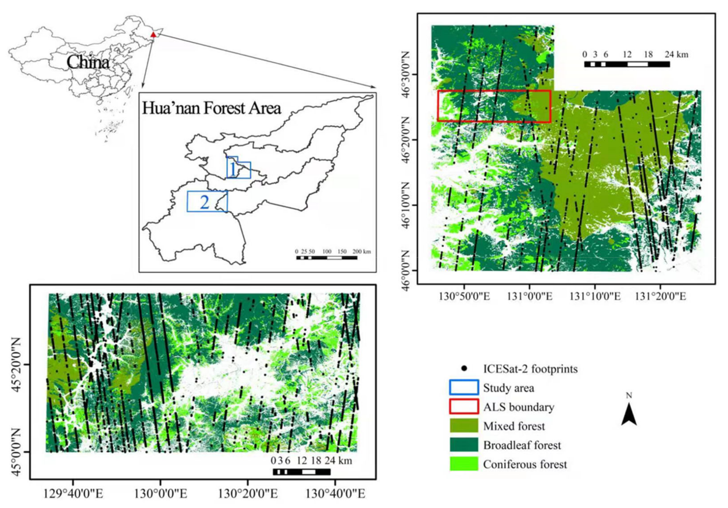
Figure 1. ICESat-2 footprints in Area 1 and Area 2, and distributions of coniferous forest, brodleaf forest, mixed forest in two study areas. (The blue polygon and rectangle denote study areas. The footprints of ICESat-2 are depicted by black dots. The red rectangle denotes the ALS data coverage area).
Remotesensing 14 00364 g001
Figure 2. A flowchart of the proposed method.
Remotesensing 14 00364 g002
Figure 3. Correlations between the validation samples and predicted forest canopy heights by RF. (a) WF, (b) CF, (c) BF, (d) MF.
Remotesensing 14 00364 g003
Figure 4. Correlations between the validation samples and predicted forest canopy heights by GBDT. (a) WF, (b) CF, (c) BF, and (d) MF.
Remotesensing 14 00364 g004
Figure 5. Sub-regions representing CF, BF, MF, and their enlarged Google images. (A) Coniferous forest, (B) Broadleaf forest and (C) Mixed forest.
Remotesensing 14 00364 g005
Figure 6. The histograms of predicted canopy heights and RH95 metric of samples in three sub-regions. (a) Coniferous forest, (b) Broadleaf forest, and (c) Mixed forest.
Remotesensing 14 00364 g006
Figure 7. The 3D map of forest canopy height obtained by the RF method for Area 1 (a) and ranges of predicted canopy heights for CF, BF, and MF (b).
Remotesensing 14 00364 g007
Figure 8. Cross-comparison between the h 90 metric of ALS and predicted forest canopy heights by RF.
Remotesensing 14 00364 g008
Figure 9. Spatial analysis for predicted forest canopy height map and GEDI-derived forest canopy height map in Area 1. (ad) represent predicted forest canopy height map, GEDI-derived forest canopy map, frequency histogram for canopy height difference, and distributions for canopy height difference with 250 m resolution).
Remotesensing 14 00364 g009
Figure 10. The optimal variables for each forest type and importance score for each variable in descending order. (a) Coniferous forest, (b) broadleaf forest, and (c) mixed forest.
Remotesensing 14 00364 g010
Figure 11. Correlations between variables for each optimal set. (a) CF, (b) BF, and (c) MF. Color bar indicates the correlation score.
Remotesensing 14 00364 g011
Table 1. The main vertical structure metrics within one segment from the ATL08 product.
Canopy Height MetricsDescription
h_max_canopyRelative maximum of individual canopy heights.
h_mean_canopyRelative mean of individual canopy heights.
h_min_canopyRelative minimum of individual canopy heights.
RH90/RH95/RH98Height metrics calculated at 90/95/98 percentiles.
Table 2. Independent variables selected for the modelling process. (The first, second, and third columns correspond to the category, name, and explanation of the variable).
TypesFeaturesDescriptionReference
Biophysical FeaturesLAILeaf area index, reflecting the density, structure, and growth of vegetation.[17]
FAPARFraction of absorbed photosynthetically active radiation, representing growth state of vegetation.[17]
FCOVERFraction of vegetation cover, quantifying the spatial extent of vegetation.[17]
Vegetation IndicesRVINIR/R, distinguishing vegetation/non vegetation areas.[16]
EVI2.5 × ((NIR-R)/(NIR + 6 × R − 7.5 × B + 1)), analyzing the changes of vegetation, especially describing the differences of vegetation in a specific climate zone.[16]
DVINIR-R, reflecting change of vegetation coverage.[16]
MSAVI(2 × NIR + 1 − sqrt((2 × NIR + 1)2 − 8 × (NIR − R)))/2[16]
NDVI_B84(NIR − R)/(NIR + R)[17]
NDVI_B85(NIR − RE1)/(NIR + RE)[17]
NDVI_B86(NIR − RE2)/(NIR + RE2)[17]
NDVI_B87(NIR − RE3)/(NIR + RE3)[17]
NDVI_B8A4(NIR2 − R)/(NIR2 + R)[17]
NDVI_B8A5(NIR2 − RE1)/(NIR2 + RE)[17]
NDVI_B8A6(NIR2 − RE2)/(NIR2 + RE2)[17]
NDVI_B8A7(NIR2 − RE3)/(NIR2 + RE3)[17]
Texture Featuresndvi_ContrastContrast provided by Grey Level Co-occurrence Matrix, making use of spatial information inherent in images for image classification.[12]
ndvi_EntropyEntropy provided by Grey Level Co-occurrence Matrix, making use of spatial information inherent in images for image classification.[12]
ndvi_GLCM VarianceGLCM Variance provided by Grey Level Co-occurrence Matrix, making use of spatial information inherent in images for image classification.[12]
/VVBackscatter value extracted from VV-polarization image, penetrating forest, and interacting with branches.[12]
VHBackscatter value extracted from VH-polarization image, penetrating forest, and interacting with branches.[17]
Topographic
Information
elevationElevation extracted from DEM, closely relating to the distribution and growth of vegetation.[17]
aspectAspect extracted from DEM, closely relating to the distribution and growth of vegetation.[17]
slopeSlope extracted from DEM, closely relating to the distribution and growth of vegetation.[17]
Table 3. The calculated R and RMSE for ICESat-2 ATL08 product and metrics derived from ALS data at different spatial resolutions.
Resolution10 m30 m250 m
ALS Metric h m e a n h m e d i a n h 90 h 95 h m a x h m e a n h m e d i a n h 90 h 95 h m a x h m e a n h m e d i a n h 90 h 95 h m a x
R0.560.230.680.690.710.590.540.730.700.680.720.680.80 0.760.75
RMSE/m3.083.292.752.712.692.902.982.592.642.872.212.451.98 2.102.18
Table 4. The number of training/validation samples corresponding to WF, CF, BF, and MF for model construction (training: validation = 8:2).
TypesTraining SamplesValidation SamplesTotal
Whole forest21175302647
Coniferous forest29274366
Broadleaf forest10282581286
Mixed forest796199995
Table 5. The calculated R and RMSE for RH95 metric of sample and predicted results for Area 2.
TypesNumber of SamplesRRMSE (m)
CF11210.673.16
BF29800.503.34
MF3230.613.31
Table 6. Sum of importance scores of variables corresponding to “Vegetation Indices”, “Topographic Information”, “Biophysical Variables”, “Texture Features”, and “VV&VH” for CF, BF, and MF.
CFBFMF
Vegetation Indices0.450.670.57
Topographic Information0.210.330.18
Biophysical Variables0.1300.10
Texture Features0.0900.08
VV&VH0.1200.07
Publisher’s Note: MDPI stays neutral with regard to jurisdictional claims in published maps and institutional affiliations.