Comparison of Winter Wheat Extraction Methods Based on Different Time Series of Vegetation Indices in the Northeastern Margin of the Qinghai–Tibet Plateau: A Case Study of Minhe, China

Abstract

The northeastern margin of the Qinghai–Tibet Plateau (QTP) is an agricultural protection area in China’s new development plan, and the primary region of winter wheat growth within QTP. Winter wheat monitoring is critical for understanding grain self-sufficiency, climate change, and sustainable socioeconomic and ecological development in the region. However, due to the complex terrain and high altitude of the region, with discontinuous arable land and the relatively low level of agricultural development, there are no effective localization methodologies for extracting and monitoring the detailed planting distribution information of winter wheat. In this study, Sentinel-2A/B data from 2019 to 2020, obtained through the Google Earth Engine platform, were used to build time series reference curves of vegetation indices in Minhe. Planting distribution information of winter wheat was extracted based on the phenology time-weighted dynamic time warping (PT-DTW) method, and the effects of different vegetation indices’ time series and their corresponding threshold parameters were compared. The results showed that: (1) the three vegetation indices—normalized difference vegetation index (NDVI), normalized differential phenology index (NDPI), and normalized difference greenness index (NDGI)—maintained high mapping potential; (2) under the optimal threshold, >88% accuracy of index identification for winter wheat extraction was achieved; (3) due to improved extraction accuracy and resulting boundary range, NDPI and its corresponding optimal parameter (T = 0.05) performed the best. The process and results of this study have certain reference value for the study of winter wheat planting information change and the formulation of dynamic monitoring schemes in agricultural areas of QTP.

1. Introduction

Wheat is a widely grown cereal worldwide, and its caryopsis is a staple for humankind [1,2,3]. Accordingly, any changes in its distribution and yield are of great significance to anthropogenic sustainability and survival; however, due to climate change, extreme weather, and socioeconomic development, the uncertainty surrounding crop planting distribution and yield is increasing, forcing regional food security issues to the front stage [4,5,6]. To address these issues, enhancement of crop planting information extraction and monitoring is essential, and could provide data that would form a basis for the formulation of polices to avert potential food crises.

Compared to field surveys, remote sensing technologies offer the ability to quickly obtain spatial distribution information of surface objects across a continuous time series and, thus, are commonly employed in the fields of crop planting identification and monitoring, and fruitful results have been obtained [7,8]. For the extraction of winter wheat information via remote sensing, methods are mainly divided into three categories: machine learning [9,10,11], time series vegetation indices [12,13,14], and classification via interpretation models [15,16,17].

Machine learning is an algorithm that can automatically analyze datasets and obtain rules to be used for predictions [18]. With the advancement of computational ability and the development of massive data processing technology, machine learning algorithms have been widely integrated into data mining and prediction applications across various industries. With respect to extracting winter wheat planting information from remote sensing data, methods range from the earlier supervised classification techniques to more recent deep learning approaches. The most common classification methods include decision tree classifications, random forest, BP artificial neural networks, and convolutional neural networks [9,19,20,21]. Machine learning methods are advantageous considering their high accuracy and wide applicability; however, they often serve as a “black-box” method; the resulting rules for obtaining the results are often too complex or concealed to be readily interpreted. In addition, they rely heavily on training samples (particularly deep learning algorithms), and the sample sizes demanded are large. Sample acquisition requires considerable labor and financial resources, with a relatively low cost performance. Although historic samples can be obtained through visual interpretation by professionals, the resulting sample accuracy is dependent upon professional ability. Therefore, machine learning is suitable for research and applications that are supported by good data and samples.

The remote sensing interpretation model uses algorithms to analyze the characteristics—texture, color, spectra—of different objects in remote sensing data for classification. Commonly used models for winter wheat interpretation have included a normalized difference vegetation index (NDVI) threshold and decision tree classification models [15,16,17]. Remote sensing interpretation models are advantageous, owing to their high extraction accuracy, sole requirement of data interpretation, and frequent data collection; however, each crop requires a spectral interpretation model or signature for different data resources, which are difficult to establish in areas with relatively weak research foundations.

Time series refer to the trends of a changing variable over equal time intervals. Theoretically, a certain static feature maintains a relatively stable time series trend [22]. Based on this principle, the time series of remote sensing-derived vegetation indices have attracted considerable interest and have successfully been used to identify winter wheat due to its significantly distinct growth or phenological features when compared to other land objects [12,13,23]. This highlights the advantages of time series vegetation indices, including wide applicability, small sample size requirements, high identification accuracy, and strong universality and extensibility.

However, with the improvement of the temporal and spatial resolution of remote sensing data, big modern remote sensing data have placed computational restrictions on all the three types of extraction methods above. For example, a machine learning algorithm processes massive amounts of remote sensing data and large sample data and completes the “join” between sample and data; thus, computational limits are reached quickly, and crashes are common [24,25]. Time series of vegetation indices require continuous remote sensing imagery, and a wide range of crop distribution areas to accurately identify phenological differences [12]. The remote sensing interpretation model requires the computer to process the input remote sensing data quickly and in real time. Fortunately, cloud computing technologies provide a possible solution to this problem, and the Google Earth Engine (GEE) Cloud Platform has been applied by many scholars for remote sensing big data processing, helping to reduce local data storage and computing pressures [26,27]. For example, Xiao et al. [28] evaluated the application potential of Sentinel-1/2 data in rice mapping over the Hangjiahu Plain in China based on the GEE, whereas He et al. [29] extracted winter wheat and winter rape from 119 landscape images by using the GEE. Yang et al. [30] used the GEE to monitor winter wheat in Shandong, China according to Sentinel-1/2 data. Accordingly, remote sensing data processing and crop information extraction can be carried out through relatively simple programming techniques, currently providing one of the most promising remote sensing technology applications available [29].

Indeed, remote sensing extraction of winter wheat planting information has a strong foundation in both methodologies and supporting platforms, as numerous references exist for dynamic monitoring by governments and industries; however, the above discussions and research on monitoring methods and platforms are mainly focused on conventional planting areas or other major grain-producing regions, with low altitudes and relatively mild climates [11,12,25]. Accordingly, in the high-altitude and cold border areas, due to the small scale of production, the contribution of grain output to the global output can be ignored, and few research activities have focused on the grain production, including extraction and monitoring of winter wheat information based on remote sensing technologies. Actually, the agricultural activities in the high-altitude and cold border areas play a major role in regional grain self-sufficiency, detection of climate change, and research on sustainable socioeconomic and ecological development.

The northeastern margin of the Qinghai–Tibet Plateau (QTP) is one of the main agricultural areas in the QTP and primarily refers to the Hehuang Valley, as a whole, and even smaller components. The northeastern margin marks the transition zone from the northeastern QTP to the Loess Plateau. With an average altitude > 3000 m, the plateau continental climate characteristics are significant. Nevertheless, it serves as the northwestern border zone for winter wheat cultivation in China. Planting wheat across river valleys ensures grain self-sufficiency for the QTP population, of about 10 million. Accordingly, changes in winter wheat planting distribution in the region can serve as an indicator of regional climate and agricultural structure change. However, recent field investigations by agricultural administration departments and with farmers have revealed that the winter wheat planting area has been decreasing annually, with frequent occurrences of extreme weather/climate events, seed degradation, pest and disease, intensified human–wildlife conflict as a result of the Chinese government’s ecological protection strategy, and low returns compared to other industries, in notable contrast to the predictions of potential expansion under a global warming background. Therefore, the main grain planting information presented here about winter wheat in the northeastern margin of QTP is vital for the prediction of future regional food security, climate change, socioeconomic growth, and environmental sustainability. However, the detailed planting distribution information of winter wheat in the region is not clear, and corresponding operational extraction and monitoring of methodologies are also lacking.

To address the above issue, remote sensing methods for extracting winter wheat in the northeastern margin of QTP are discussed. Specifically, this study selected Minhe (Qinghai, China) in the northeastern margin of QTP as the study area. Based on its socio-economic development, data support and the cost-effective, widely applied time series vegetation index method was selected as a guideline, and the optimal vegetation index and corresponding threshold parameters were selected for extracting winter wheat distribution information. In detail, a winter wheat sample reference curve was constructed using Sentinel-2 A/B data of the GEE platform, and the identification effects of different vegetation indices combined with the phenology time-weighted dynamic time warping (PT-DTW) algorithm were compared to obtain the optimal predictive indices and corresponding model (i.e., algorithm) parameters for distribution mapping. The findings of the present study could lay a foundation for the development of methods for the extraction of winter wheat planting information in the northeastern margin of QTP, and provide a technical reference for subsequent remote sensing monitoring efforts for other important agricultural products.

2. Materials and Methods

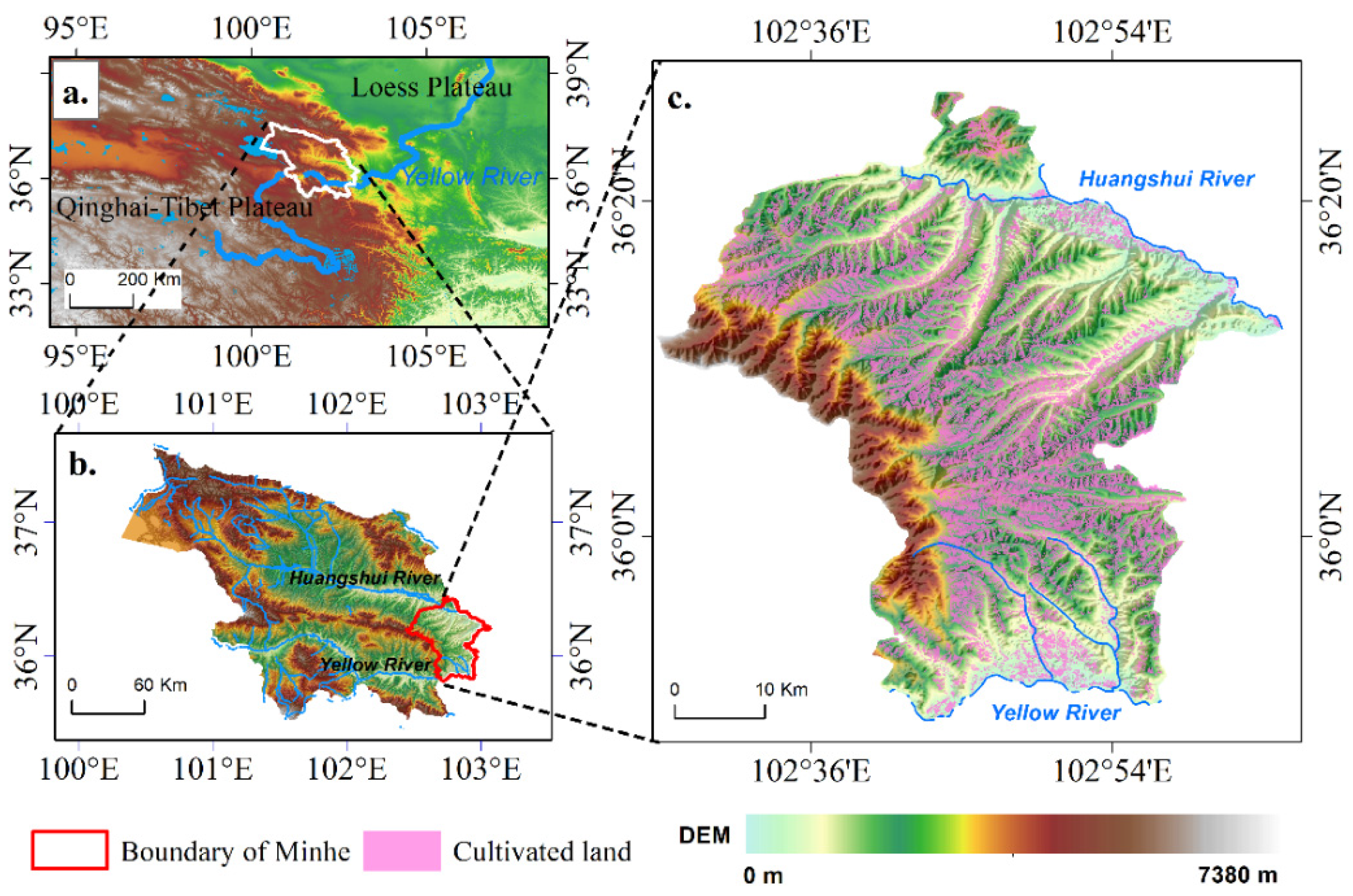
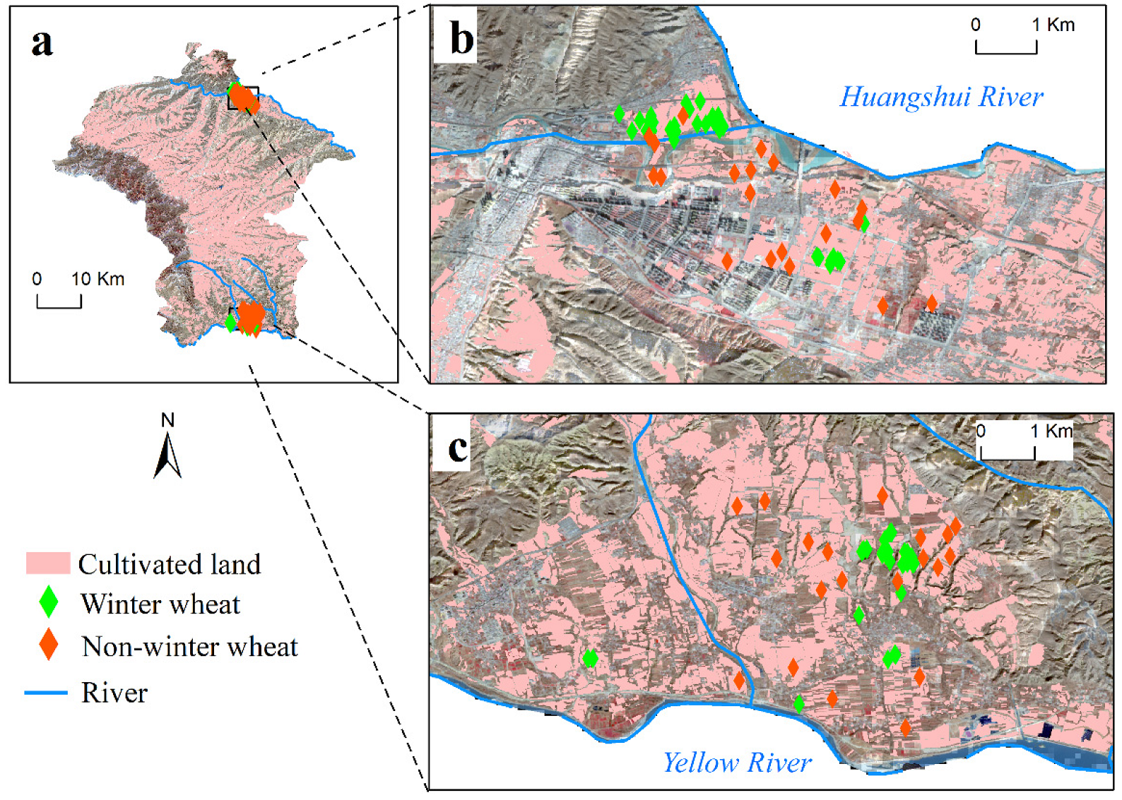
2.1. Study Area

Minhe is located in the Hehuang Valley, northeastern QTP, under the jurisdiction of Qinghai Province, China. It comprises a portion of the transition zone from the Loess Plateau to the QTP (Figure 1) and maintains a typical plateau continental climate. The terrain is high in the northwest, low in the southeast, and high mountains dominate the southwest. The maximum and minimum altitudes are 4220 m and 1650 m, respectively, with the average altitude being 2100–2500 m. Ravines and mountainous territory overlap, creating complex terrain. The fertile cultivated land area, suitable for planting wheat, corn, rapeseed, etc., accounts for approximately 24% of the total land area [31]. Yellow and Huangshui River Valleys are suitable for planting winter wheat due to better hydrothermal conditions in these areas [31]. Since 1958, winter wheat has been planted in the region, and large-scale promotion has been gradually realized; however, due to the influence of unstable natural conditions, such as climate change and extreme weather/climatic events, harvest yield fluctuates greatly [32]. Compared with growth in the main producing area of China, the winter wheat growth in the same phenological period in this region is significantly weaker, with relatively longer growth periods (sowing in mid-September, maturity in mid-to-late July of the following year) [12]. At present, regional winter wheat is mainly distributed in the Hehuang Valley, namely, the Yellow and Huangshui River Valleys. However, data from the government statistics department and interviews with farmers revealed that the proportion of winter wheat planting area to grain crops planting area has shrunk sharply in recent years in Minhe. Elsewhere, it has been shown that under the influence of global warming, the suitable planting area of winter wheat in Minhe has expanded [32]. Accordingly, it is necessary to conduct localized research on winter wheat planting information extraction in the region, which could facilitate an examination of change in agricultural structure under the influence of climate change, socioeconomic transition, and ecological protection.

2.2. Data

The distribution of cultivated land in Minhe is scattered and discontinuous, under the influence of topographic and climatic factors, and the land plot area is small; therefore, when considering the spatiotemporal resolution of the image and cost-effectiveness of the application, Sentinel 2A/B satellite data (

Table 1. Sentinel 2A/B remote sensing data parameters.

Band Number	1	2	3	4	5	6	7	8	8a	9	10	11	12
Central wavelength (nm)	433.9/ 442.3	496.6/ 492.1	560 /559	664.5/ 665	703.9/ 703.8	740.2/ 739.1	782.5/ 779.7	835.1/ 833	864.8/ 864	945/ 943.2	1373.5/ 1376.9	1613.7/ 1610.4	2202.4/ 2185.7
Spatial resolution (m)	60	10	10	10	20	20	20	10	20	60	60	20	20

) were selected for the analysis here, owing to its relatively high resolution and 5-day revisit period, which are conducive to the synthesis of crop growth curves with dense time series. Because GEE has built-in Sentinel 2 datasets that have undergone partial pre-processing steps, it is readily available for extractions of bottom-of-atmosphere corrected reflectance information. Accordingly, this study obtained all 678 pre-processed Sentinel 2A/B data scenes across Minhe from 25 August 2019 to 30 July 2020.

Administrative and cultivated land spatial distribution data were also used in this study, with the data on administrative divisions coming from the 1:1,000,000 national basic geographic database [33], and cultivated land data were obtained from within the research group of the authors.

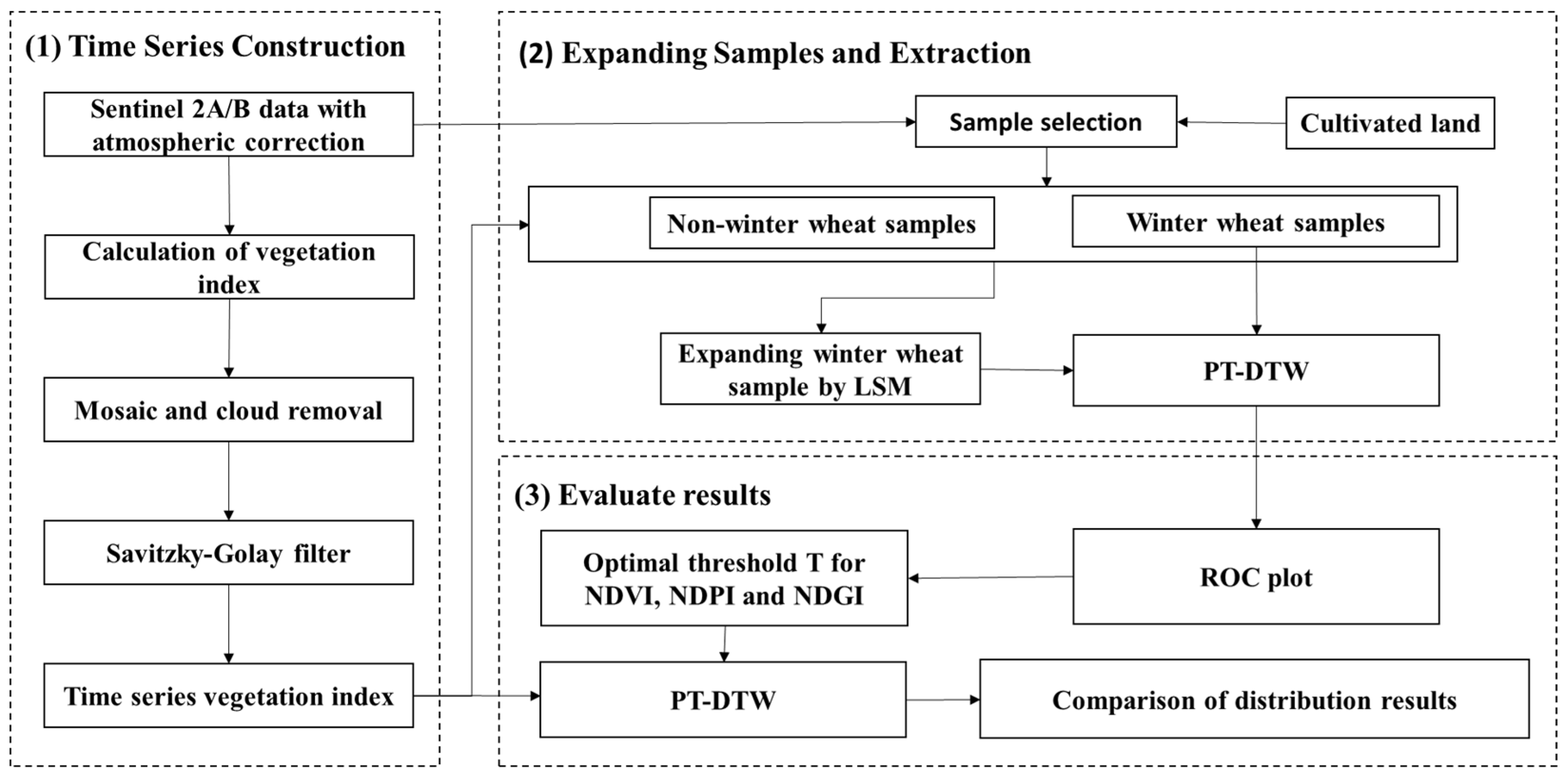
2.3. Technical Scheme

Based on Sentinel 2A/B data, a comparative study on winter wheat identification methods was conducted here using the PT-DTW method combined with the vegetation indices of time series in GEE. The conceptual diagram of the processes used is shown in Figure 2 and includes three primary components: (1) constructing high-quality time series vegetation indices, (2) expanding the winter wheat sample set and setting an extraction threshold, and (3) evaluating the precision of winter wheat identification from different vegetation indices. The details are as follows.

2.3.1. Time Series Construction

Initially, based on the 678 obtained atmosphere-corrected images, the NDVI, normalized differential phenology index (NDPI), and normalized difference greenness index (NDGI) were calculated. Subsequently, the time series of images were mosaicked using the quality mosaic algorithm every 10 days and clipped based on the administrative division of Minhe. Lastly, the vegetation indices were combined into a time sequence, and a Savitzky–Golay (SG) filter was used to obtain a high-quality data time series for each pixel.

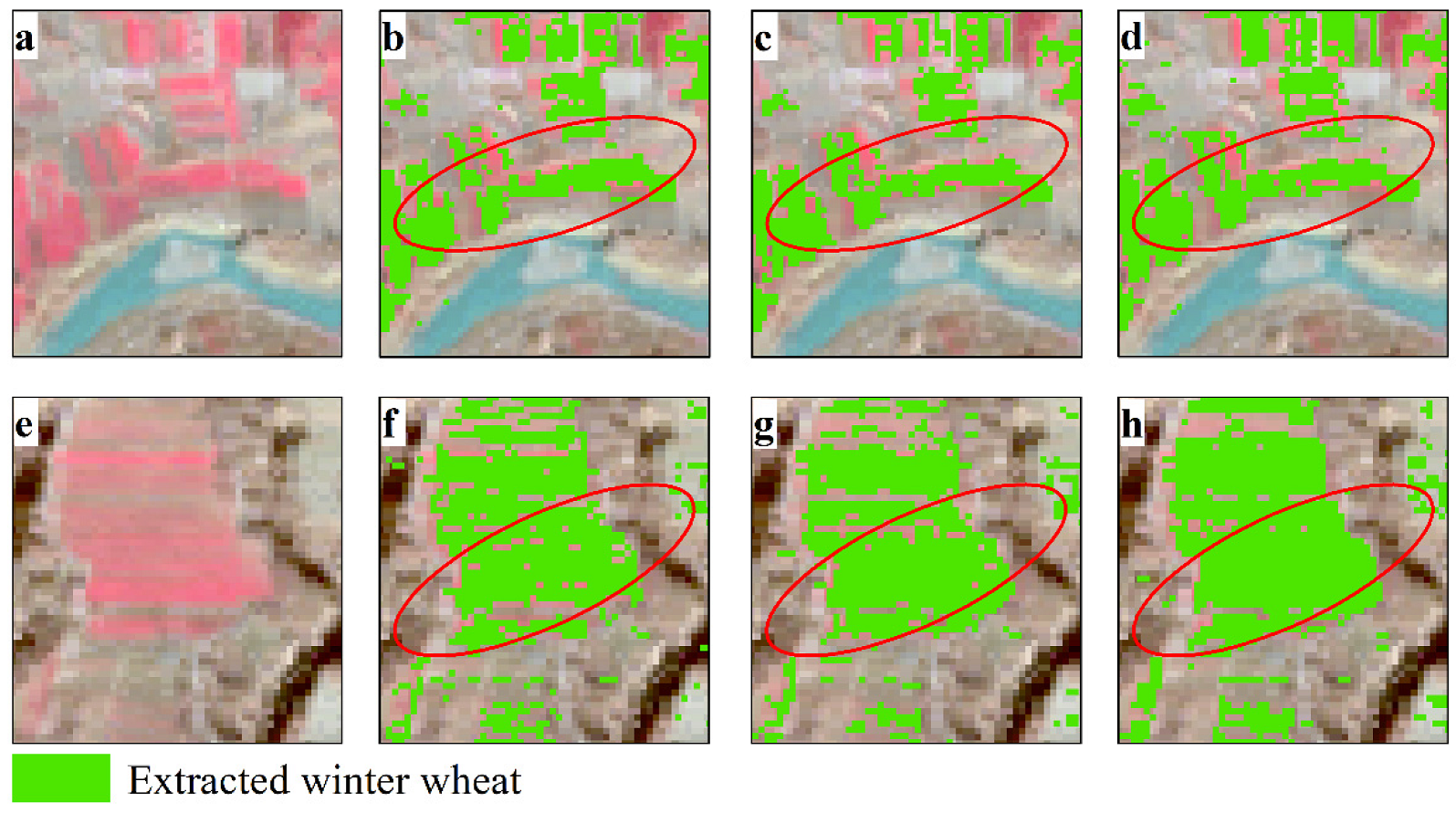
2.3.2. Expanding Samples and Extraction

According to the characteristics of winter wheat in the imagery, an SG filtered time series of vegetation indices and sample points of presence/absence were selected based on the distribution of cultivated land. Next, a median value of 30 winter wheat samples was used to construct the reference curve. A linear spectral mixed model (LSM) was used to expand upon the reference curve dataset (4500 presence and 4500 absence samples) using 30 presence and 10 absence samples. Taking cultivated land as the reference, a threshold T value was set between 0 and 0.3 for each index and was tested according to the sample dataset combined with PT-DTW. Finally, the receiver operating characteristic (ROC) curve was created according to the experimental results, and another 30 presence and 30 absence samples.

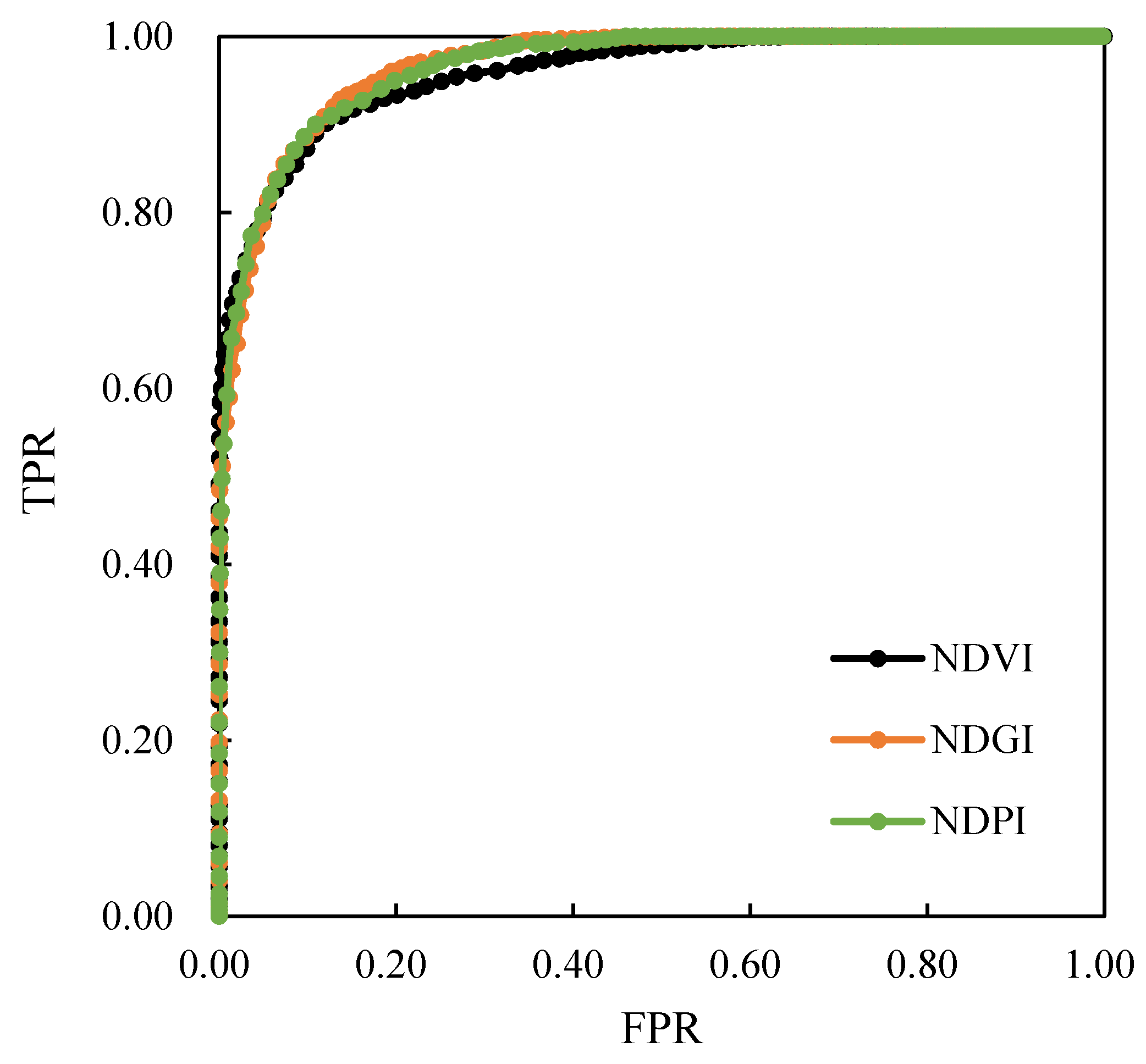
2.3.3. Accuracy Assessment via ROC and Optimal T

The optimal threshold value for each vegetation index was selected by analyzing ROC. The optimal T for each vegetation index was applied to identify winter wheat and the mapping effects of each vegetation index were assessed.

2.4. Vegetation Indices

The vegetation indices composed of the spectral reflectance of vegetation can help control the influence of signal attenuation when electromagnetic waves pass through the atmosphere [34]. Accordingly, they are widely used to evaluate vegetation cover and growth status as well as improve the precision of remote sensing monitoring of vegetation (e.g., crops) growth or yield estimates [35,36,37]. NDVI, NDGI and NDPI are common vegetation indices used to characterize vegetation distribution. NDVI (Equation (1)) is the most widely used vegetative evaluation index and is suitable for dynamic monitoring in early and middle growth stages [34,38]. Furthermore, NDVI has been extensively studied for its extraction potential of winter wheat [17,39,40]. However, NDVI is affected by snow cover and soil background. NDGI and NDPI are two vegetation cover indices that eliminate the influence of these factors, and can better reflect the greenness characteristics of vegetation in the case of snow cover. To be specific, NDPI was designed to enhance the comparison between vegetation and background (i.e., it is soil and snow insensitive), while minimizing the differences between backgrounds (Equation (2)) [41]; thus, it often maintains a higher accuracy for identifying wheat growth information than NDVI and has an enhanced vegetation index (EVI) [12,42]. NDGI is an analysis index based on the linear spectral mixture model proposed by Yang et al. [43] (Equation (3)). It essentially removes the influence of snow on the vegetation index and has shown good response effects on sparsely vegetated or cropland areas. There are many cases in which the two indices have been verified using small samples of phenological observation sites and carbon flux sites, and there are a few cases in which the accuracy of the indices has been evaluated on a large spatial scale, but this also demonstrates their application potential.

$$\mathrm{NDVI}=\frac{B_{nir}-B_r}{B_{ndr}+B_r}$$

(1)

$$\mathrm{NDPI}=\frac{B_{nir}-\left(0.74\times B_r+0.26\times B_{swir}\right)}{B_{nir}+\left(0.74\times B_r+0.26\times B_{swir}\right)}$$

(2)

$$\mathrm{NDGI}=\frac{0.65\times B_{nir}+0.35\times B_g-B_r}{0.65\times B_{nir}+0.35\times B_g+B_r}$$

(3)

where $B_g$, $B_r$, $B_{nir}$, and $B_{swir}$ correspond to the green, red, near-infrared, and mid-infrared bands, respectively, equating to B3, B4, B8, and B11 of Sentinel 2 data, respectively.

As described in Section 2.1, the topography of Minhe is complex, with land cover seasonally dominated by snow. Winter wheat cultivation is discontinuous and sparse in winter. No study has proposed a vegetation index suitable for winter wheat extraction in this region. Accordingly, NDVI, NDPI, and NDGI were selected for the identification of winter wheat to identify the optimal index and corresponding threshold parameters.

2.5. Mosaic and Cloud Removal Algorithm

Although Sentinel-2A/B scene data are 290 km wide, the inconsistent coverage range of each image required the mosaicking of multiple scenes for complete study area coverage. In addition, cloud masks for affected images are necessary across all remote sensing applications. Using the quality mosaic function of GEE, it was found that when NDVI was designated as the quality band, image mosaic and cloud removal effects were more precise compared to when NDPI or NDGI were employed. Thus, mosaicking was conducted accordingly, using the quality mosaic function of GEE, cloud removal was carried out through the mosaic cloud removal method directly, and a phase mosaic, cloud free image was synthesized with a step length of 10 days.

2.6. Savitzky–Golay Filter

Owing to inherent uncertainties in satellite image acquisition, remote sensing data, including the created time series here, maintain certain levels of temporal noise. Filtering time series data is, thus, a necessary process for constructing reliable crop growth curves based on vegetation indices [44]. The present study directly selected Savitzky–Golay (SG) filtering as the smoothing method for NDVI, NDPI, and NDGI time series, based on similar successful applications for vegetation time series [45,46,47] and winter wheat identification [12,48,49].

In essence, SG filtering relies on the least square fitting of local high order polynomials to obtain weights, and then calculates weighted averages in order to smooth curves. Assuming that there are 2n + 1 terms, t times of fitting, the calculation formula of any SG filtered value is as follows:

$$Y_j={\displaystyle \sum }_{i=-n}^n\left(C_i\ast Y_{i+j}\right),\hspace{1em}(t<2n+1)$$

(4)

where Y_j is the result after SG filtering. When the given higher order polynomial is determined, the weights of the terms are also determined. When the polynomial is a three-order and five-term fit, the calculation formula of the intermediate term can be simplified to:

$$V_0=-\frac{3}{35}\ast Y_{-2}+\frac{12}{35}\ast Y_{-1}+\frac{17}{35}\ast Y_0+\frac{12}{35}\ast Y_1-\frac{3}{35}\ast Y_2$$

(5)

where V₀ is the result of SG filtering of the middle term, Y₋₂ and Y₋₁ are the former 2 and 1 terms of the middle term, respectively, Y₁ and Y₂ are the after 1 and 2 terms of the middle term, respectively.

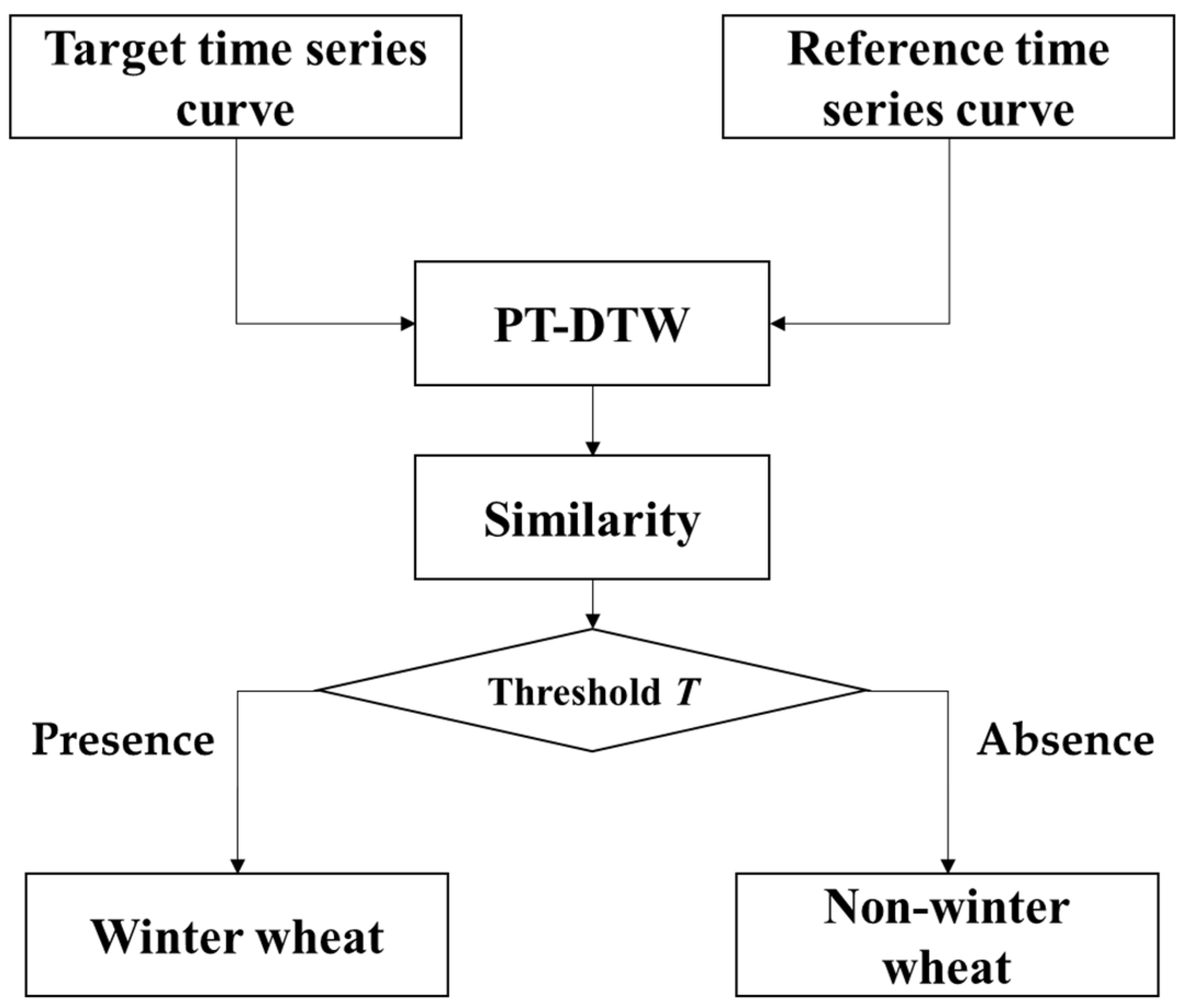
2.7. PT-DTW Algorithm

PT-DTW is an improved algorithm for winter wheat recognition based on the dynamic time warping (DTW) algorithm [12]. DTW is a widely used method for measuring the similarity between two time series of different lengths [50,51,52], although it is notably limited by excessive distortion. To address this issue, Dong et al. [12] added a time–distance penalty (M) [12,53] for calculating the DTW similarity matrix (d) to enhance the phenological weight of winter wheat and, thus, highlight its dual growth peak characteristics (Figure 3). Thus, the PT-DTW method was implemented for winter wheat extraction in the North China Plain by combining the NDPI time series. The results indicated good verification accuracy [12], and the relatively small training sample size requirements led to the selection of the PT-DTW method for combining NDVI, NDPI, and NDGI time series data as an alternative identification scheme for winter wheat in Minhe.

For the specific calculation process of PT-DTW, it is assumed that there are two curves, Q = (q₁, q₂, q₃, …, q_m), R = (r₁, r₂, r₃, …, r_m), with the same number of nodes in the event sequence. Q and R are the curves of target event sequence and reference time series, respectively. For each element in the matrix (6): $6=\left|q_i-R_j\right|+M_{i,j},i\in \left[1,m\right],j\in \left[1,m\right]$, $M_{i,j}=\frac{1.0}{1+e^{-0.1\ast \left(\ast T\left|i-j\right|-100\right)}}$

$$d_{n,m}=\left(\begin{array}{cccc}{d}_{1,1}& d_{1,2}& \dots & d_{1,m}\\ d_{2,1}& d_{2,2}& ..& d_{2,m}\\ \dots & \dots & \dots & \dots \\ d_{m,1}& d_{m,2}& \dots & d_{m,m}\end{array}\right)$$

(6)

The minimum cost path from d_1,1 to d_m,n is solved in the matrix, and then the sum of the points value on the path multiplied by the weight W_i is the PT-DTW values of Q and R. The formula for calculating this value is as follows:

$$\mathrm{PT}-\mathrm{DTW}=d_{1,1}+{\displaystyle \sum }_{i=1}^{m-1}\min \left(d_{i+1,j+1},d_{i,j+1},d_{i+1,j}\right)\ast W_i$$

(7)

2.8. Accuracy Evaluation

ROC is a graphic method for representing the accuracy of binary classification models [54], creating a two-dimensional graph of the relationship between the true positive rate (TPR) (Equation (8)), and the false positive rate (FPR; Equation (9)). As early as 1989, Spackman [55] examined the value of utilizing the relatively simple ROC curves for evaluating and comparing classification algorithms. In an ROC diagram, each point on the curve represents the corresponding classification result of a group of parameters, where the closer the point is to the upper left corner, the more accurate the results, (i.e., high TPR and low FPR). Points under different thresholds are connected to form the ROC curves. Notably, if the ROC curve representing one vegetation index is above the curves of other indices, it indicates the superiority of this index within the given application. A binary classification model (i.e., presence, absence) was employed in the present study, and the ROC curve could thus be used to evaluate the performance of different vegetation indices for winter wheat identification and classification results. The formulas for each evaluation index of ROC are presented in Equations (8)–(10):

$$\mathrm{TPR}=\frac{TP}{TP+FN}\times 100\%$$

(8)

$$\mathrm{FPR}=\frac{FP}{FP+TN}=100-\frac{TN}{TN+FP}\times 100\%$$

(9)

$$\mathrm{ACC}=\frac{TP+TN}{TP+FP+FN+TN}\times 100$$

(10)

where TP is the number of correct classifications of positive samples, FN is the number of incorrect classifications of positive samples, FP is the number of incorrect classifications of negative samples, TN is the number of correct classifications of negative samples, and ACC is the accuracy rate.

3. Process and Results

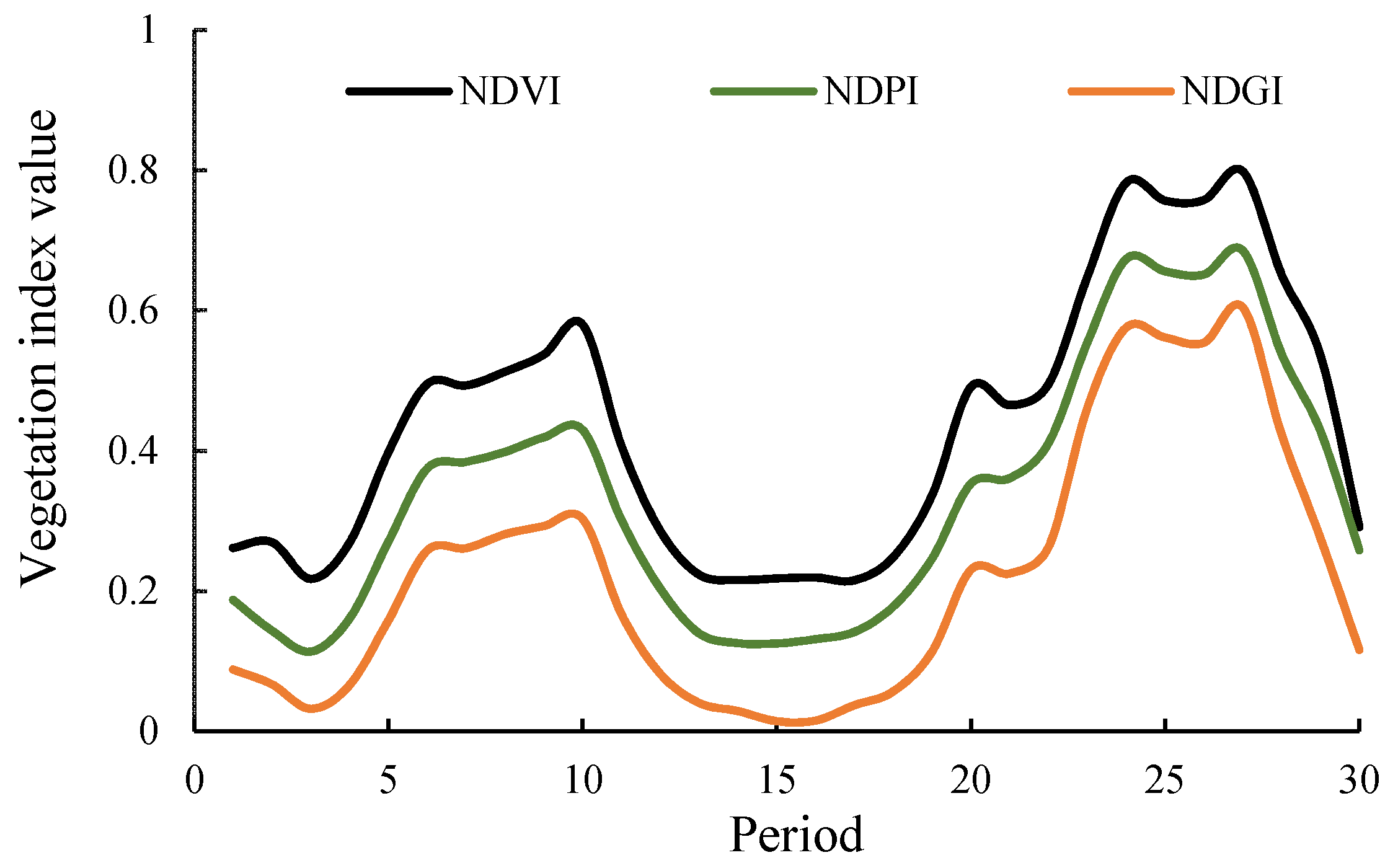
3.1. Time Series of Vegetation Indices

According to the conceptual design, the construction of the time series of vegetation indices for winter wheat in Minhe included three main processes:

(1)

The vegetation indices were first calculated for all images. In GEE, the image expression interface was used to program and carry out the vegetation index algorithms according to Equations (1)–(3) by calling the 678 atmospheric corrected images covering Minhe from the Sentinel 2A/B dataset; afterwards, NDVI, NDPI, and NDGI were obtained.

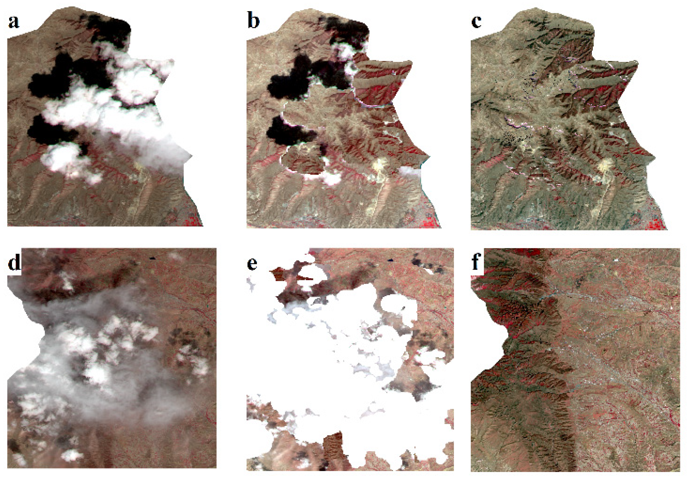
(2)

Using the quality mosaic function within GEE, a 10-day time step, and NDVI was designated as the quality band, the multi-temporal images were mosaicked and cloud cover was removed, resulting in a total of 34 time series images. The corresponding bands of the three vegetation indices were then extracted from the mosaics and combined into three sets of time series vegetation index images for constructing a high-quality index curve.

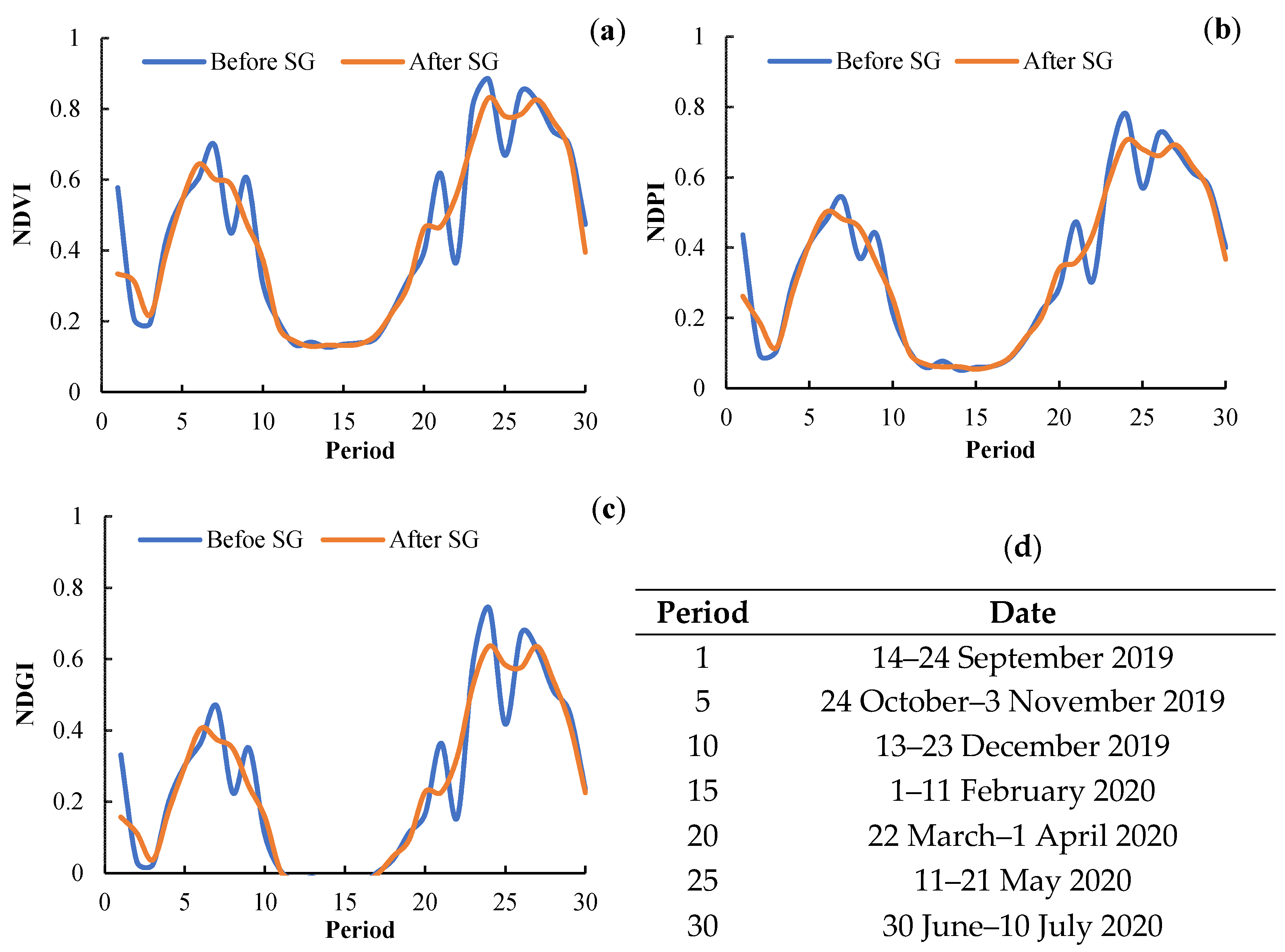
(3)

According to the SG filtering principle [45], the filter function of three times 5-point fitting was programmed in GEE to smooth the time series of indices. This program eliminated the data of the initial and final periods, resulting in 30 time series images from 14 September 2019 to 7 October 2020.

Figure 4 shows the comparison of vegetation indices pre- and post-SG filtering of a single and randomly selected winter wheat sample point. The results indicate that the influence of noise on the time series of data was visibly weakened by filtering; that is, the impact of abrupt changes in the vegetation index value caused by atmospheric interactions were reduced, resulting in more accurate vegetation index values at each time step. In addition, winter wheat in Minhe is sown in mid-to-late September and enters the heading stage in early June (Figure 4) [39]. The vegetation indices of winter wheat at the emergence and tillering stages increased rapidly within the time series, whereas other vegetation present either decreased or remained unchanged. The vegetation indices decreased rapidly at the mature stages, while the other forms of vegetation remained either constant or increased slowly. Two characteristic phenological periods were selected: 3–6 and 27–30, corresponding to 4 October–13 November 2019 and 31 May–10 July 2020, respectively.

3.2. Selection of Reference Curve and Threshold T

Parameter setting of the PT-DTW algorithm is the key to extracting winter wheat information via the fusion of the vegetation indices time series. Parameter setting involves three steps: (1) Obtaining the median reference curve of winter wheat and expanding the samples; (2) Setting the key phenology weight of winter wheat. The research results of Dong et al. [12] showed that winter wheat recognition effects were superior when equal-weight values were assigned to data of the key phenological period, that is, the sum of weights of the key phenological period was 1.0, and data of other phenological periods were not involved in the calculation, as was employed here; (3) Selecting the extraction threshold T for winter wheat.

3.2.1. Sample Selection

Winter wheat sample selection is critical to constructing the reference curves of vegetation indices time series. Here, in the field investigation, winter wheat samples were not obtained during growing season of 2019 to 2020; thus, the manual interpretation of archived remote sensing data was conducted. Cultivated land data were taken as the reference, and the sample points of winter wheat were obtained according to its bright red standard false color spectral characteristics when it overwintered and typical bimodal time series of vegetation indices during growth. The potential distribution range of winter wheat was estimated according to the changing characteristics of accumulated temperature with altitude in the study area and the availability of natural water systems or other sources capable of ensuring irrigation [31]. Lastly, in the Huangshui and Yellow River Valleys, 60 winter wheat sample points and 40 non-winter wheat sample points were selected (Figure 5,

Table A1. Sample point location information.

No. Winter Wheat	Longitude (°)	Latitude (°)	No. Winter Wheat	Longitude (°)	Latitude (°)
1	102.8321991	36.34012101	31	102.8215339	36.33791838
2	102.8329072	36.33851354	32	102.8492914	36.31909747
3	102.8314678	36.33938116	33	102.8471242	36.31906289
4	102.829043	36.33893176	34	102.8487979	36.31800324
5	102.8256956	36.33860335	35	102.8502784	36.31847005
6	102.8250305	36.33805023	36	102.8673894	35.88064135
7	102.8225199	36.33917374	37	102.8657318	35.88057615
8	102.822198	36.34008982	38	102.8669388	35.88134548
9	102.8205458	36.3394503	39	102.8664976	35.88251362
10	102.8278629	36.3411096	40	102.8627154	35.88264401
11	102.8628656	35.88213114	41	102.8499259	36.31859709
12	102.8622648	35.88223545	42	102.8468145	36.31923679
13	102.8597081	35.88306055	43	102.848924	36.31855179
14	102.8588498	35.88267807	44	102.8538681	36.3241419
15	102.8645378	35.8653727	45	102.8313483	36.33999818
16	102.8632644	35.86459453	46	102.8303329	36.33885767
17	102.8636554	35.8858618	47	102.8323928	36.33806257
18	102.866505	35.88077895	48	102.8295158	36.34228171
19	102.8632671	35.88265455	49	102.8274237	36.34199652
20	102.8674006	35.88131822	50	102.8174997	36.34039149
21	102.8658503	35.88072301	51	102.8223066	36.33788167
22	102.8660586	35.88259989	52	102.8193938	36.33784398
23	102.8623315	35.88262329	53	102.858364	35.87200979
24	102.8635761	35.88107597	54	102.8654506	35.87580491
25	102.8638681	35.88585876	55	102.8591318	35.88298318
26	102.8483604	35.85708426	56	102.8676366	35.88072546
27	102.8644224	35.86548096	57	102.8672289	35.88178599
28	102.821937	36.33926221	58	102.8626812	35.88465212
29	102.8259041	36.33777124	59	102.8129411	35.86476349
30	102.8256573	36.33652671	60	102.8138048	35.86478088
No. Non-Winter Wheat	Longitude (°)	Latitude (°)	No. Non-Winter Wheat	Longitude (°)	Latitude (°)
1	102.8225883	36.33116338	21	102.8687295	35.88501014
2	102.8370508	36.3320277	22	102.8623717	35.89202697
3	102.8335317	36.31854326	23	102.8379958	35.89028862
4	102.8566631	36.31186933	24	102.8426306	35.89112303
5	102.8639587	36.31221515	25	102.8555911	35.87784088
6	102.8383095	35.86103466	26	102.8531878	35.8826394
7	102.8685648	35.86169548	27	102.8499263	35.88430838
8	102.8661999	35.85309907	28	102.852072	35.87624131
9	102.8445903	35.88152691	29	102.8691725	35.88154746
10	102.8746066	35.88693187	30	102.8648703	35.87768775
11	102.8716616	35.88003489	31	102.849542	36.32919305
12	102.8736786	35.88191256	32	102.853576	36.3262888
13	102.8732709	35.88556345	33	102.8529752	36.32449088
14	102.8474047	35.86326588	34	102.8346074	36.3315786
15	102.8539707	35.85797924	35	102.8237069	36.33095629
16	102.8427819	36.31772324	36	102.8385939	36.33521086
17	102.8400031	36.31880382	37	102.8404308	36.33316065
18	102.8416768	36.31988438	38	102.822755	36.33605531
19	102.8482343	36.32258948	39	102.8219181	36.33702329
20	102.8369678	36.32863987	40	102.8269607	36.34009998

); among them, 30 presence and 10 absence samples were randomly selected to construct the reference curves of vegetation indices and expand the experimental samples, whereas all remaining samples were used for verification.

3.2.2. Vegetation Indices Reference Curves

The median of the sampled curves was selected as a reference of winter wheat time series that are neither biased towards the winter wheat growing well nor growing poorly. Accordingly, the median of each vegetation index from 30 randomly selected winter wheat samples was taken as the corresponding time series reference (i.e., standard curve; Figure 6).

3.2.3. Selection of Threshold T

In essence, the PT-DTW value is used to measure the similarity between a specific time series curve and the reference curve for winter wheat, whereas a smaller value indicates greater similarity. The T value accuracy directly determines the accuracy of extraction as it represents the threshold between winter wheat and non-winter wheat. In principle, threshold T values should be obtained based on sample data, but an insufficient sample size can lead to incongruencies between the determined and optimal thresholds. Accordingly, the linear spectral mixing (LSM) [12] model can develop a large number of sample datasets using a relatively small set of sample data. Therefore, the LSM model used in this study generated mixed vegetation index curves from the median reference curve, and any two others from 30 randomly selected winter wheat samples and 10 randomly selected non-winter wheat samples. A total of 4500 positive and 4500 negative samples were generated (those with winter wheat composition > 50% were considered positive samples). Then, the minimum PT-DTW values of each sample and the 30 winter wheat samples were calculated. In the analysis, the T value of the 30 winter wheat samples were <0.3; therefore, a corresponding range of T value was set from 0.0 to 0.3, with a change in step size of 0.001. Lastly, based on the extended sample dataset and cultivated land, winter wheat across Minhe was extracted based on different threshold T values and time series of vegetation indices.

Figure 7 shows the ROC plot based on the results of the above process and Equations (8) and (9). The figure indicates that all three vegetation indices have the potential to accurately identify winter wheat. For FPR ≤ 5%, the TPRs of the three indices were nearly equal, indicative of their similar ability within the low FPR range. When the FPR > 5%, the TPR of NDVI was slightly lower than that of NDPI or NDGI, indicating that the latter two vegetation indices, which successfully minimized the noise associated with background soil and snow cover, is superior to the former during the identification of winter wheat.

To determine the optimal threshold T value, the distance between each point on the ROC plot and the coordinate point (0, 1) was calculated, and the threshold represented by the point with the smallest distance was considered optimal for each of the vegetation indices (

Table 2. Optimal thresholds (T), error indices, and accuracy.

VI	T	TPR	FPR	ACC
NDVI	0.060	76.66%	0.0%	88.33%
NDPI	0.050	83.33%	0.0%	91.67%
NDGI	0.051	80.00%	0.0%	90.00%

). The accuracy was verified based on the remaining 30 winter wheat presence and absence samples. From the ROC curve, the FPRs of the three indices were all zero while maintaining a high TPR (>75%), indicating that the selection result of the optimal threshold value was reasonable. The ACC for NDPI was the best, followed by NDGI and NDVI. As smaller optimal threshold values indicate a more accurate identification potential for winter wheat, NDPI (T = 0.050) was identified as the top predictor of winter wheat presence in the analyses here.

Partial distribution results of winter wheat in Minhe were then extracted using the optimal threshold values in Table 2 (Figure 8). Overall, the spatial distributions of winter wheat based on the three vegetation indices were good; however, notable differences emerged at higher levels of detail. In the discontinuous growing area (Figure 8a), the corresponding winter wheat distribution maps based on the three indices captured this pattern (Figure 8b–d), whereas in the more continuous areas (Figure 8e), the results based on NDVI remained irregular (Figure 8f) and those based on NDPI and NDGI were relatively contiguous (Figure 8g,h). Notably, the resulting boundary range based on NDGI was largest, followed by NDVI. Accordingly, NDPI was also optimal according to the extracted spatial distribution results.

4. Discussion and Conclusions

To optimize the method of extraction of winter wheat based on the time series of vegetation indices and corresponding threshold parameters for the Hehuang Valley agricultural area in QTP, Minhe (Qinghai, China) was selected as the research area. With the support of the GEE platform and Sentinel 2A/B data, atmosphere-corrected image data were used to calculate the NDVI, NDPI, and NDGI of winter wheat in the 2019–2020 growing season, and mosaicking was performed based on the mosaic cloud removal method. A high-quality time series of the vegetation indices was obtained by SG filtering after ordering chronologically. Lastly, after selecting points of true winter wheat presence through visual interpretation, extension of samples by the LSM algorithm, and based on the PT-DTW algorithm, analytical optimization of the winter wheat extraction method was carried out using ROC curves.

In the above processes, the calculation of each vegetation index using the atmospherically corrected data helped reduce the atmospheric effects and more accurately reflected the vegetative growth condition on the ground.

When mosaicking and masking cloud cover, the quality mosaic algorithm provided by GEE was adopted to retain the pixel value with the highest quality among all mosaic data. A comparison with the results of another cloud removal algorithm specifically for Sentinel 2A/B data provided by GEE (Figure 9) showed that although the latter can achieve reasonable cloud removal effects, it simply excludes cloud and shadow pixels, resulting in missing pixels during multi-phase image mosaics when all images involved in mosaicking are missing pixels at the same location (Figure 9b,e). The former technique (adopted in the present research) was applied due to its advantage in the form of the ability to maximize retention of high-quality pixels (Figure 9c,f) while removing cloud cover as much as possible for subsequent processing; however, this method could produce false high-quality pixels due to cloud cover over a long time series, increasing the resulting error. Therefore, mosaicking and cloud removal fusion were carried out in this method to reduce the error transmission caused by the two processes being carried out separately to some extent, and also ensured the integrity of the result data. In addition, the study area was located in middle/high latitudes and in the temperate continental monsoon climate zone, with sunnier days with less cloud cover. The probability of the inability to synthesize an optical fusion image in the short time interval due to cloud cover is small. In order to obtain a good phenological curve and reduce the noise of time series, fusion images were constructed with a time-interval of 10 days in this study. However, in areas with more cloudy and rainy weather, such as the Mediterranean climate region, optical remote sensing images in winter could be highly affected by weather conditions and cloud presence and, thus, it may be difficult to obtain short-time-interval fusion images. Therefore, determination of the maximum acceptable time-interval and how the accuracy changes by increasing/decreasing this time interval requires further study.

In terms of noise removal of the vegetation index time series curve, there is a general consensus that SG filtering is more capable of weakening time series noise compared to asymmetric Gaussian filtering, double-logic filtering, or Fourier filtering [45]. In the present study, the SG filter used five time period units to smoothen the data, improving stability and reliability of the time series of the vegetation indices. Therefore, the data and preprocess methods in this study are somewhat reliable.

In terms of setting the phenological option weight, this study referred to Dong et al. [12] and only selected data of characteristic phenological periods to set the weight and participate in the calculation. Compared with using all phenology data in the calculation, the amount of data and computation were greatly reduced, and the complex weight determination process was also reduced. For sample handling, sample points for winter wheat were selected following visual interpretation, and the reference curve constructed from the sample median ensured that it would neither favor winter wheat with good growth nor with poor growth. Accordingly, referring to previous studies [12,56], the LSM model was used to expand the sample dataset as well as to ensure that the generated positive sample data were always near the median reference curve and were roughly consistent with actual sample data. The identification accuracy of winter wheat based on these extended samples was also consistent with those derived from previous studies [12,56]; however, the experimental results of the sample dataset expanded via the LSM model were used in threshold selection, which may be notably different from those based on a field-derived samples. Therefore, it is necessary to make up for the absence of field investigation samples in subsequent analyses.

The winter wheat phenological weight used in the present study was directly referenced from research on the main winter wheat producing areas in central and eastern China [12]. The terrain of the present research area is complex, with discontinuous winter wheat planting, whereas the central and eastern planting regions of China are relatively flat, with contiguous winter wheat planting. Therefore, subsequent research should compare the characteristics and growth differences of winter wheat between the study area and the main production areas in the central and eastern regions of China, optimizing models for local phenological weight to improve the identification accuracy.

The T value directly determines the accuracy of the extraction result. For the identification and extraction of winter wheat, different vegetation indices correspond to different optimal thresholds. Compared with existing studies [12,56], there are slight differences in the threshold of the NDPI index between the plain area and the northeastern part of the QTP. In the results of this study, as the threshold increases, TPR increases at an obvious speed. However, when TPR continues to rise to a certain extent, FPR increases also become obvious, and each adjustment of the threshold is accompanied by great changes in the results. Therefore, the determination of the threshold is an important process of the technical scheme, and the determination of the localization threshold is particularly important in the generalization.

In summary, based on ROC and the spatial distribution results of extracted winter wheat, all three vegetation index time series, combined with the PT-DTW method examined, had the potential to extract spatial information on winter wheat. Under the optimal threshold, the accuracy of winter wheat extraction according to the three-index identification was >88%. The classification effects of NDVI were notably poorer than those of NDPI and NDGI, indicating that the indices that have minimized the background effects of soil and snow are more suitable for winter wheat identification. Although NDPI did not perform any better than NDGI in terms of the reliability of extracted winter wheat lands, it is advantageous, owing to its improved extraction accuracy and yielded boundary range. This showed that the vegetation indices that reduced the influence of soil and snow background at the same time were slightly better than those that reduced the influence of snow background alone, in terms of the overall accuracy of winter wheat extraction. Accordingly, NDPI and its corresponding optimal parameter (T = 0.05) performed optimally. However, as mentioned above, there are uncertainties in this study, such as image fusion time interval, sample processing, phenological period selection and weight determination, and threshold determination. For the extraction of winter wheat, if the study area changes, the results of corresponding parameters in this study may also change. The localization parameter determination based on this scheme is necessary in the generalization, although these parameters may vary very little from region to region. Of course, if it is to extract other crops, the specific extraction scheme should be designed separately, given the spectral and phenological differences between them and winter wheat.

Based on the above result, the planting area of winter wheat in Minhe during the 2019–2020 growing season, extracted in the present study, was 431.79 ha. According to recent field investigations by agricultural administration departments and interviews with farmers in the present study, farmer willingness to plant wheat has decreased. In addition, winter wheat planting area exhibits a decreasing trend. Based on the experiences of the interviewees, the winter wheat planting area extracted in this study is potentially similar to the actual planting area. The actual planting area of winter wheat in the 2019–2020 growing season was not obtained in this study; therefore, subsequent studies should consider verifying the results obtained in the present study.

References

1. Shiferaw, B.; Smale, M.; Braun, H.; Duveiller, E.; Reynolds, M.; Muricho, G. Crops that feed the world 10. Past successes and future challenges to the role played by wheat in global food security. Food Secur. 2013, 5, 291–317. [Google Scholar] [CrossRef] [Green Version]
2. Curtis, T.; Halford, N.G. Food security: The challenge of increasing wheat yield and the importance of not compromising food safety. Ann. Appl. Biol. 2014, 164, 354–372. [Google Scholar] [CrossRef] [PubMed] [Green Version]
3. Vashisth, A.; Krishanan, P.; Joshi, D.K. Multi stage wheat yield estimation using different model under semiarid region of India. Int. Arch. Photogramm. 2019, XLII-3-W6, 263–267. [Google Scholar] [CrossRef] [Green Version]
4. Mäkinen, H.; Kaseva, J.; Trnka, M.; Balek, J.; Kersebaum, K.C.; Nendel, C.; Gobin, A.; Olesen, J.E.; Bindi, M.; Ferrise, R.; et al. Sensitivity of European wheat to extreme weather. Field Crop. Res. 2018, 222, 209–217. [Google Scholar] [CrossRef]
5. Porter, J.R.; Xie, L.; Challinor, A.J.; Cochrane, K.; Howden, S.M.; Iqbal, M.M.; Lobell, D.B.; Travasso, M.I. Food security and food production systems. In Climate Change 2014: Impacts, Adaptation, and Vulnerability. Part A: Global and Sectoral Aspects. Contribution of Working Group II to the Fifth Assessment Report of the Intergovernmental Panel on Climate Change; Field, C.B., Barros, V.R., Dokken, D.J., Mach, K.J., Mastrandrea, M.D., Bilir, T.E., Chatterjee, M., Ebi, K.L., Estrada, Y.O., Genova, R.C., et al., Eds.; Cambridge University Press: Cambridge, UK; New York, NY, USA, 2014; pp. 485–533. [Google Scholar]
6. Vannoppen, A.; Gobin, A.; Kotova, L.; Top, S.; De Cruz, L.; Vīksna, A.; Aniskevich, S.; Bobylev, L.; Buntemeyer, L.; Caluwaerts, S.; et al. Wheat yield estimation from NDVI and regional climate models in Latvia. Remote Sens. 2020, 12, 2206. [Google Scholar] [CrossRef]
7. Hatfield, P.L.; Pinter, P.J., Jr. Remote sensing for crop protection. Crop Prot. 1993, 12, 403–413. [Google Scholar] [CrossRef]
8. Viña, A.; Gitelson, A.A.; Rundquist, D.C.; Keydan, G.; Leavitt, B.; Schepers, J. Monitoring maize (Zea mays L.) Phenology with remote sensing. Agron J. 2004, 96, 1139–1147. [Google Scholar] [CrossRef]
9. Fang, P.; Zhang, X.; Wei, P.; Wang, Y.; Zhang, H.; Liu, F.; Zhao, J. The classification performance and mechanism of machine learning algorithms in winter wheat mapping using Sentinel-2 10 m resolution imagery. Appl. Sci. 2020, 10, 5075. [Google Scholar] [CrossRef]
10. Wang, Y.; Zhang, Z.; Feng, L.; Du, Q.; Runge, T. Combining multi-source data and machine learning approaches to predict winter wheat yield in the conterminous United States. Remote Sens. 2020, 12, 1232. [Google Scholar] [CrossRef] [Green Version]
11. Song, D.; Zhang, C.; Yang, X.; Li, F.; Han, Y.; Gao, S.; Dong, H. Extracting winter wheat spatial distribution information from GF-2 image. J. Remote Sens. 2020, 24, 596–608. [Google Scholar]
12. Dong, Q.; Chen, X.; Chen, J.; Zhang, C.; Liu, L.; Cao, X.; Zang, Y.; Zhu, X.; Cui, X. Mapping winter wheat in North China using Sentinel 2A/B data: A method based on phenology-time weighted dynamic time warping. Remote Sens. 2020, 12, 1274. [Google Scholar] [CrossRef] [Green Version]
13. Yang, Y.; Tao, B.; Ren, W.; Zourarakis, D.P.; El Masri, B.; Sun, Z.; Tian, Q. An improved approach considering intraclass variability for mapping winter wheat using multitemporal MODIS EVI Images. Remote Sens. 2019, 11, 1191. [Google Scholar] [CrossRef] [Green Version]
14. Zhong, L.; Hu, L.; Zhou, H.; Tao, X. Deep learning-based winter wheat mapping using statistical data as ground references in Kansas and northern Texas. U.S. Remote Sens. Environ. 2019, 233, 111411. [Google Scholar] [CrossRef]
15. Huang, Q.; Wu, W.; Dend, H.; Zhang, L. Study on planting areas, extraction of remote sensing and monitoring of crop growth of winter wheat and rice in Jiangsu Province in 2009. Jiangsu Agric. Sci. 2010, 6, 508–511. [Google Scholar]
16. Li, Y.; Chen, X.; Duan, H.; Shen, Y. Application of multi-source and multi-temporal remote sensing data in winter wheat identification. Geogr. Geo-Inf. Sci. 2010, 26, 47–49. [Google Scholar]
17. Qin, Y.; Zhao, G.; Jiang, S.; Jinnan, C.; Yan, M.; Baihong, L.; Guochen, X.; Jiguang, H. Winter wheat yield estimation based on high and moderate resolution remote sensing data at county level. Trans. Chin. Soc. Agric. Engin. 2009, 25, 118–123. [Google Scholar]
18. Yang, T.; Wang, Q.; Liu, Y.; Wan, Y.; Nie, X. A review of application of machine learning in wireline logging formation evaluation. J. Oil Gas Technol. 2020, 42, 27–38. [Google Scholar] [CrossRef]
19. Cui, R.; Liu, Y.; Fu, J. Estimation of winter wheat biomass using visible spectral and BP based artificial neural networks. Spectrosc. Spect. Anal. 2015, 35, 2596–2601. [Google Scholar]
20. Feng, M.; Yang, W.; Zhang, D.; Cao, L.; Wang, H.; Wang, Q. Monitoring planting area and growth situation of irrigation-land and dry-land winter wheat based on TM and MODIS data. Trans. Chin. Soc. Agric. Engin. 2009, 25, 103–109. [Google Scholar]
21. He, Y.; Wang, C.; Jia, H.; Chen, F. Research on extraction of winter wheat based on random forest. Remote Sens. Technol. Appl. 2018, 33, 1132–1140. [Google Scholar]
22. Yang, H.; Pan, Z.; Bai, W. Review of time series prediction methods. Comput. Sci. 2019, 46, 21–28. [Google Scholar]
23. Song, Y.; Wang, J. Mapping winter wheat planting area and monitoring its phenology using sentinel-1 backscatter time series. Remote Sens. 2019, 11, 449. [Google Scholar] [CrossRef] [Green Version]
24. Shi, F.; Gao, X.; Yang, L.; He, L.; Jia, W. Research on typical crop classification based on HJ-1A hyperspectral data in the Huangshui River Basin. Remote Sens. Technol. Appl. 2017, 32, 206–217. [Google Scholar]
25. Zhang, J.; Zhang, X.; Tian, L.; Zhang, Q. The support vector machine method for RS images’ classification in northwest arid area. Sci. Surv. Mapp. 2017, 42, 49–52. [Google Scholar] [CrossRef]
26. Mutanga, O.; Kumar, L. Google Earth Engine applications. Remote Sens. 2019, 11, 591. [Google Scholar] [CrossRef] [Green Version]
27. Wu, B.; Zhang, X.; Zeng, H.; Zhang, M.; Tian, F. Big data methods for environmental data. Bull. Chin. Acad. Sci. 2018, 33, 804–811. [Google Scholar]
28. Xiao, W.; Xu, S.; He, T. Mapping paddy rice with Sentinel-1/2 and phenology-, object-based algorithm—An implementation in Hangjiahu Plain in China using GEE platform. Remote Sens. 2021, 13, 990. [Google Scholar] [CrossRef]
29. He, Z.; Zhang, M.; Wu, B.; Xing, Q. Extraction of summer crop in Jiangsu based on Google Earth Engine. J. Geo-Inf. Sci. 2019, 21, 752–766. [Google Scholar]
30. Yang, A.; Zhong, B.; Wu, J. Monitoring winter wheat in ShanDong province using Sentinel data and Google Earth Engine platform. In Proceedings of the 10th International Workshop on the Analysis of Multitemporal Remote Sensing Images (MultiTemp), IEEE, Shanghai, China, 5–7 August 2019. [Google Scholar]
31. Zhao, B.; Zhao, D. Regional drought risk of winter wheat in Minhe County Qinghai Province. Sci. Technol. Qinghai Agri. Forest. 2018, 3, 18–23. [Google Scholar]
32. Li, W.; Jiao, S.; Li, R. Effects of climate change on winter wheat in Minhe County. Sci. Technol. Qinghai Agri. Forest. 2018, 112, 6–11. [Google Scholar]
33. National Catalogue Service for Geographic Information. 1:1,000,000 National Basic Geographic Database. Available online: https://www.webmap.cn/commres.do?method=result100W (accessed on 11 January 2021).
34. Tian, Q.; Min, X. Advances in study on vegetation indices. Adv. Earth Sci. 1998, 13, 10–16. [Google Scholar]
35. Miao, Z.; Liu, Z.; Wang, Z.; Song, K.; Du, J.; Zeng, L. Dynamic monitoring of vegetation fraction change in Jilin Province based on MODIS NDVI. Remote Sens. Technol. Appl. 2010, 25, 387–393. [Google Scholar]
36. Liu, X.; Pan, Y.; Zhu, X.; Li, S. Spatiotemporal variation of vegetation coverage in Qinling-Daba Mountains in relation to environmental factors. Acta Geogr. Sinica 2015, 70, 705–716. [Google Scholar]
37. Wang, X.; Hou, X. Variation of normalized difference vegetation index and its response to extreme climate in coastal China during 1982–2014. Geogr. Res. 2019, 38, 807–821. [Google Scholar]
38. Costa, L.; Nunes, L.; Ampatzidis, Y. A new visible band index (vNDVI) for estimating NDVI values on RGB images utilizing genetic algorithms. Comp. Elect. Agric. 2020, 172, 105334. [Google Scholar] [CrossRef]
39. Dong, C.; Zhao, G.; Qin, Y.; Wan, H. Area extraction and spatiotemporal characteristics of winter wheat–summer maize in Shandong Province using NDVI time series. PLoS ONE 2019, 14, e226508. [Google Scholar] [CrossRef] [PubMed] [Green Version]
40. Li, F.; Ren, J.; Wu, S.; Zhao, H.; Zhang, N. Comparison of regional winter wheat mapping results from different similarity measurement indicators of NDVI time series and their optimized thresholds. Remote Sens. 2021, 13, 1162. [Google Scholar] [CrossRef]
41. Wang, C.; Chen, J.; Wu, J.; Tang, Y.; Shia, P.; Black, T.A.; Zhu, K. A snow-free vegetation index for improved monitoring of vegetation spring green-up date in deciduous ecosystems. Remote Sens. Environ. 2017, 196, 1–12. [Google Scholar] [CrossRef]
42. Tian, J.; Zhu, X.; Shen, Z.; Wu, J.; Xu, S.; Liang, Z.; Wang, J. Investigating the urban-induced microclimate effects on winter wheat spring phenology using Sentinel-2 time series. Agric. Forest Meteorol. 2020, 294, 108153. [Google Scholar] [CrossRef]
43. Yang, W.; Kobayashi, H.; Wang, C.; Shend, M.; Chen, J.; Matsushita, B.; Tang, Y.; Kim, Y.; Bret-Hartei, M.S.; Zona, D.; et al. A semi-analytical snow-free vegetation index for improving estimation of plant phenology in tundra and grassland ecosystems. Remote Sens. Environ. 2019, 228, 31–44. [Google Scholar] [CrossRef]
44. Li, R.; Zhang, X.; Liu, B.; Zhang, B. Review on methods of remote sensing time-series data reconstruction. J. Remote Sens. 2009, 13, 335–341. [Google Scholar]
45. Kai, Z.; Jönsson, P.; Jin, H.; Eklundh, L. Performance of smoothing methods for reconstructing NDVI time-series and estimating vegetation phenology from MODIS data. Remote Sens. 2017, 9, 1271. [Google Scholar] [CrossRef] [Green Version]
46. Chen, J.; Jönsson, P.; Tamura, M.; Gua, Z.; Matsushita, B.; Eklundh, L. A simple method for reconstructing a high-quality NDVI time-series data set based on the Savitzky–Golay filter. Remote Sens. Environ. 2004, 91, 332–344. [Google Scholar] [CrossRef]
47. Wang, L.; Qi, F.; Shen, X.; Huang, J. Monitoring multiple cropping index of Henan Province, China based on MODIS-EVI time series data and Savitzky-Golay Filtering algorithm. Comput. Model. Eng. Sci. 2019, 119, 331–348. [Google Scholar] [CrossRef] [Green Version]
48. Wang, M.; Zhang, X.; Huang, Y.; Hong, C.; Zhang, Z.; Huang, X.; Zeng, J.; Tang, J.; Zhang, R. Monitoring of winter wheat and summer corn phenology in Xiong’an new area based on NDVI time series. In Proceedings of the International Conference on Wireless Communication, Network and Multimedia Engineering (WCNME 2019), Guilin, China, 21–22 April 2019; Atlantis Press: Guilin, China, 2019; p. 21. [Google Scholar]
49. Zhuo, W.; Huang, J.; Gao, X.; Ma, H.; Huang, H.; Su, W.; Meng, J.; Li, Y.; Chen, H.; Yin, D. Prediction of winter wheat maturity dates through assimilating remotely sensed leaf area index into crop growth model. Remote Sens. 2020, 12, 2896. [Google Scholar] [CrossRef]
50. Chen, H.; Liu, C.; Sun, B. Survey on similarity measurement of time series data mining. Cont. Decis. 2017, 32, 1–11. [Google Scholar]
51. Tu, G.; Geng, X. Research and implementation of similarity computation for spatiotemporal trajectories. Comp. Digit. Engin. 2020, 48, 1114–1120. [Google Scholar] [CrossRef]
52. Wang, H.; Gong, Y.; Liu, W. Study on spatial-temporal multiscale adaptive method of gesture recognition. Comp. Sci. 2017, 44, 287–291. [Google Scholar]
53. Maus, V.; Camara, G.; Cartaxo, R.; Sanchez, A.; Ramos, F.M.; de Queiroz, G.R. A time-weighted dynamic time warping method for land-use and land-cover mapping. IEEE J. Select. Topics Appl. Earth Obs. Remote Sens. 2016, 9, 3729–3739. [Google Scholar] [CrossRef]
54. Fawcett, T. An introduction to ROC analysis. Pattern Recogn. Lett. 2006, 27, 861–874. [Google Scholar] [CrossRef]
55. Spackman, K.A. Signal detection theory: Valuable tools for evaluating inductive learning. In Proceedings of the Sixth International Workshop on Machine Learning; Elsevier: Amsterdam, The Netherlands, 1989. [Google Scholar]
56. Dong, J.; Fu, Y.; Wang, J.; Tian, H.; Fu, S.; Niu, Z.; Han, W.; Zheng, Y.; Huang, J.; Yuan, W. Early-season mapping of winter wheat in China based on Landsat and Sentinel images. Earth Syst. Sci. Data 2020, 12, 3081–3095. [Google Scholar] [CrossRef]
Figure 1. Study area locations of the Qinghai–Tibet Plateau and Minhe. (a). Location of Hehuang Valley; (b). Location of Minhe in Hehuang Valley; (c). DEM and Cultivated land distribution of Minhe (DEM: digital elevation model).
Remotesensing 14 00343 g001
Figure 2. Conceptual diagram of the process used for winter wheat identification.
Remotesensing 14 00343 g002
Figure 3. Schematic diagram of phenology time-weighted dynamic time warping (PT-DTW).
Remotesensing 14 00343 g003
Figure 4. SG filtering effects of a single sample point for (a) NDVI, (b) NDPI, (c) NDGI, and (d) the dates corresponding to period number.
Remotesensing 14 00343 g004
Figure 5. Distribution of sample points. (a). Location of sample boxes in Minhe; (b,c). Distribution of winter wheat and non-winter wheat sample points in the sample boxes.
Remotesensing 14 00343 g005
Figure 6. Reference curves for winter wheat time series of vegetation indices.
Remotesensing 14 00343 g006
Figure 7. ROC curves of each vegetation index: FPR, false positive rate; TPR, true positive rate.
Remotesensing 14 00343 g007
Figure 8. Partial distribution results of winter wheat: (ad) are the extraction results of the Huangshui Valley area (representing discontinuous winter wheat coverage); (eh) are the extraction results of the Yellow River Valley area (representing contiguous coverage); and panels from left to right are winter wheat results extracted by false color imaging, NDVI, NDPI, and NDGI, in this order.
Remotesensing 14 00343 g008
Figure 9. Phase 24: 22 April 2020 to 2 May 2020 composite: (a,d) are clouded areas in the original Sentinel images, (b,e) depict the Sentinel 2 de-clouding function built into GEE, and (c,f) are the mosaic cloud removal method employed in the present study.
Remotesensing 14 00343 g009