Article

Towards an Improved Large-Scale Gridded Population Dataset: A Pan-European Study on the Integration of 3D Settlement Data into Population Modelling

1
German Remote Sensing Data Center (DFD) of the German Aerospace Center (DLR), Oberpfaffenhofen, D-82234 Weßling, Germany
2
Center of International Earth Science Information Network CIESIN, The Earth Institute, Columbia University, Palisades, NY 10964, USA
3
WorldPop, School of Geography and Environmental Science, University of Southampton, Southampton SO17 1BJ, UK
*
Author to whom correspondence should be addressed.
Remote Sens. 2022, 14(2), 325; https://doi.org/10.3390/rs14020325
Submission received: 7 December 2021 / Revised: 6 January 2022 / Accepted: 7 January 2022 / Published: 11 January 2022
(This article belongs to the Section Urban Remote Sensing)

Abstract

:
Large-scale gridded population datasets available at the global or continental scale have become an important source of information in applications related to sustainable development. In recent years, the emergence of new population models has leveraged the inclusion of more accurate and spatially detailed proxy layers describing the built-up environment (e.g., built-area and building footprint datasets), enhancing the quality, accuracy and spatial resolution of existing products. However, due to the consistent lack of vertical and functional information on the built-up environment, large-scale gridded population datasets that rely on existing built-up land proxies still report large errors of under- and overestimation, especially in areas with predominantly high-rise buildings or industrial/commercial areas, respectively. This research investigates, for the first time, the potential contributions of the new World Settlement Footprint—3D (WSF3D) dataset in the field of large-scale population modelling. First, we combined a Random Forest classifier with spatial metrics derived from the WSF3D to predict the industrial versus non-industrial use of settlement pixels at the Pan-European scale. We then examined the effects of including volume and settlement use information into frameworks of dasymetric population modelling. We found that the proposed classification method can predict industrial and non-industrial areas with overall accuracies and a kappa-coefficient of ~84% and 0.68, respectively. Additionally, we found that both, integrating volume and settlement use information considerably increased the accuracy of population estimates between 10% and 30% over commonly employed models (e.g., based on a binary settlement mask as input), mainly by eliminating systematic large overestimations in industrial/commercial areas. While the proposed method shows strong promise for overcoming some of the main limitations in large-scale population modelling, future research should focus on improving the quality of the WFS3D dataset and the classification method alike, to avoid the false detection of built-up settlements and to reduce misclassification errors of industrial and high-rise buildings.

Graphical Abstract

1. Introduction

The human population is one of the core elements influencing sustainable development. Global socio-environmental issues such as poverty, inequality, food security, land degradation, and climate change, amongst others, can only be properly addressed with a full and clear understanding of how demographic trends and population dynamics affect (positively and negatively) the social, economic and environmental development of any given region [1,2]. On this basis, to effectively implement and monitor sustainable policies, governments, researchers and policymakers around the world need to have access to high-quality, timely, reliable and spatially explicit population data. Accurate knowledge on where and in what density humans live is essential not only to promote evidence-based decisions, but also to develop location-based strategies capable of improving the living conditions of people residing in both, rural and urban areas [3].
To respond to the increasing demand for robust population data, new global and continental geospatial datasets that describe the size, extent and spatial distribution of the human population are constantly being produced, harnessing the accelerated development of Earth Observation (EO) technologies [4,5,6,7]. State-of-the-art gridded population datasets produced through the synergies of Remote Sensing (RS) and Geographical Information Systems (GIS), such as the Gridded Population of the World (GPW) [8], the Global Human Settlement-Population (GHS-Pop) [9], the LandScan datasets [10,11], the WorldPop datasets [12], the World Settlement Footprint population (WSF-Pop) datasets [13,14], and the High-Resolution Settlement Layer (HRSL) [15] are becoming particularly popular among researchers and practitioners, who are increasingly considering them as “dominant sources of population data” [16].
Concisely, gridded population datasets complement and supplement conventional aggregated census data, including projections and estimations. They provide a detailed geographical framework that allows the integration of population data with other geospatial layers, enabling the deployment of spatial and temporal analyses at local, regional and global scales [16]. The aforementioned population datasets, for example, provide near-global to global coverage estimations of population distributions at spatial resolutions of ~1 km, ~250 m, ~100 m ~30 m and ~10 m at the equator, respectively. The majority have been produced using a “top-down” dasymetric modelling technique [17], in which population counts from census, estimates or projections stored in native census units (e.g., census blocks, townships, districts) are disaggregated into uniform georeferenced grid cells or pixels, by means of a “restrictive” or “probability” layer. Depending on the specific method used to derive these layers, dasymetric techniques can range from binary-weighted, to more complex multi-layer and statistically weighted techniques, in which different remotely sensed geospatial datasets or proxy layers (e.g., land cover, lights at night, elevation, slope, distance to roads, distance to rivers, protected areas, built-up areas, etc.) are used to determine the variations in the density and distribution of population within the administrative units [18] (see [19] for more details).
From an application point of view, gridded population datasets have been largely employed to support a wide range of research areas including urban development [20], land-use planning [21] and environmental assessments [22]. Most recently, however, topics related to disaster risk assessment [3,23,24], health studies on infectious diseases [25] and humanitarian actions [26] in particular have gained some predominance. Currently, gridded population datasets are being used for mapping populations at risk [27], plan emergency response actions [28], assess inequities in access to services [29], improve planning for equitable service delivery and plan financial budgets. The sensitivity of these applications illuminates the need for gridded population datasets to be as accurate as possible, as errors or biases in the estimation of vulnerable populations can have considerable implications, in terms of policy and decision making, as well as affect all the steps of crisis management tasks [30].
In this context, the integration of new and highly detailed built-up land datasets into large-scale population modelling frameworks has played a major role in the production of more accurate population distribution datasets [31,32]. New datasets that describe the location, characteristics and distribution of human settlements such as the High-Resolution Settlement Layer (HRSL) [15], the Global Urban Footprint (GUF) [33], the World Settlement Footprint (WSF) [34,35], the Global Human Settlement Layer (GHSL) [36], the WorldPop growth built-up models [37] and building patterns [38], the Ecopia/Maxar [39], Microsoft [40] and Google building footprints [41] datasets have proven to increase the internal quantitative and qualitative accuracy of population models up to 10–15% (based on different metrics) [15,42,43,44]. Here, accuracy refinements are mainly attributed to the relative completeness of these built-area datasets, where the identification of human settlements in rural and remote areas, in particular, has improved drastically over the years [31,43].
However, despite the advancements that these built-area and building footprint datasets have brought to the field of large-scale population modelling, current global gridded population datasets produced on the basis of these proxy layers still present some limitations, as none of them provide de facto detailed information on the functional use (residential versus non-residential) and vertical dimension of the built-up environment. This consistent lack of information has resulted in large errors of under- and overestimation in population estimates, especially in studies carried out at the local scale. For example, in the work of Thomson et al. [45], the accuracy of the GHS-Pop, GPW4v.11, LandScan, HRSL and WorldPop datasets (among other products) on slums located in Nigeria and Kenya was evaluated. The statistical results indicated that, on average, 80% of the population located in these areas was being underestimated by these datasets due to the lack of information on settlement use, building heights and building densities. Comparably, in the accuracy assessment of the WSF-Pop datasets presented by Palacios-Lopez et al. [13,14], the authors demonstrated that large overestimation errors (sometimes higher than 150%) can be present in the final products. This was especially true in urban regions, where non-residential buildings (e.g., large industrial and commercial areas) were treated as residential, and where high-rise buildings were treated identically to single houses.
With that being said, multiple local-scale studies have already shown that including building type/use and building 3D information into models of population distribution can greatly improve the accuracy in population estimations [31,46,47,48,49,50,51]. In these studies, improvements of 10% up to 20% have been reported, resulting mainly from the exclusion of non-residential areas and the inclusion of volume data, respectively. Nevertheless, information on building use/type and volume has not yet been integrated into modern large-scale population modelling due to a lack of appropriate data at/for large extents (e.g., national, continental, and global). Currently, existing research that focuses on extracting use-related semantic information of built-up structures relies on a combination of regionalized building footprints, cadastral data, LiDAR data, social media data, aerial imagery and/or commercial (and frequently expensive) very high-resolution imagery (e.g., <5 m optical data or orthoimage) [52,53,54,55,56,57], which restricts the implementation of the developed methods to the specific areas where these data are available, reliable, replicable and—more importantly—complete.
In this framework, the German Aerospace Center (DLR) has been working on the World Settlement Footprint 3D (WSF3D) [58], a temporally consistent and spatially detailed global dataset quantifying the fraction, total area, average height and total volume of building stock within settlements. The final WSF3D is processed at a 90 m spatial resolution, and according to the results of a first comprehensive technical quantitative assessment [58], it reports accuracy metrics that are fairly consistent with independent, high-resolution reference data (e.g., LiDAR derived datasets). In this study, an advanced version of the WSF3D is used which quantifies the built-up density at an improved spatial resolution of 12 m (see Section 2.2 for more details).
In light of these new developments, a question that remains open is whether the integration of the WSF3D dataset into models of population distribution can improve the quantitative accuracy of population estimates. While gridded population datasets produced on the basis of the binary and imperviousness WSF layers (2015 and 2019) have already shown some qualitative and quantitative advantages over other existing products [13,14], to the best of our knowledge, no assessment that reports on the suitability of the WSF3D dataset in the framework of large-scale top-down population modelling has been undertaken. Therefore, in this research, we examine the utility of the WSF3D dataset as a single proxy for top-down, large-scale population modelling. This examination was carried out following a two-step approach briefly described as follows:
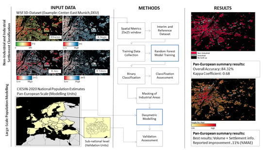
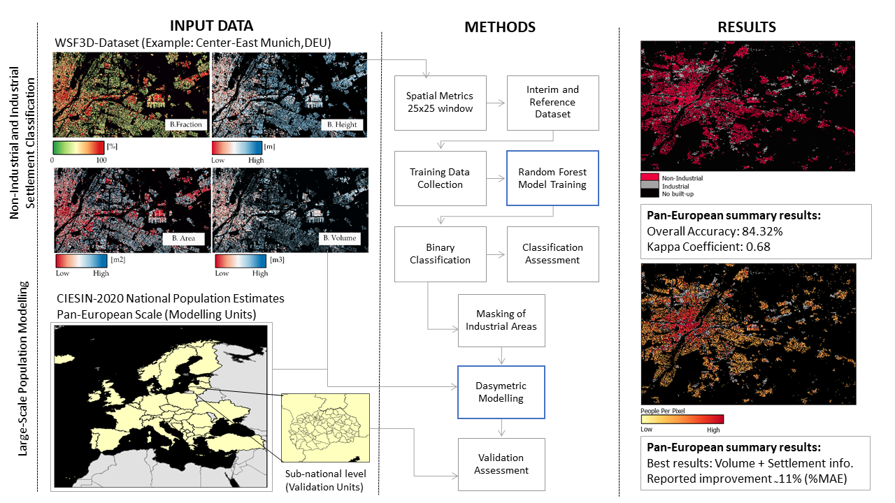
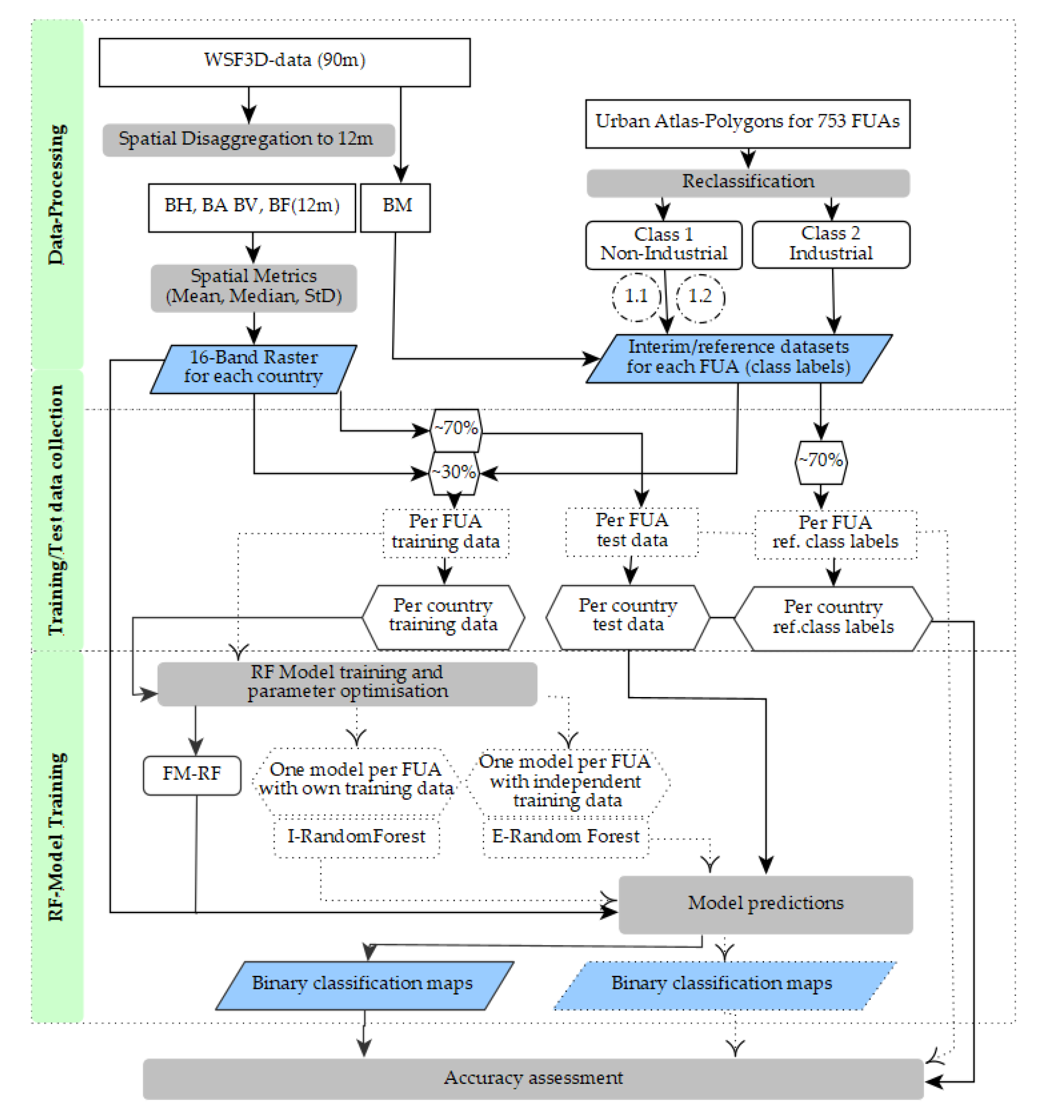
  • In the first step, we investigate if the WSF3D dataset can be used to effectively identify and eliminate large industrial/commercial areas from the built-up environment, which in the past have been reported as major sources of under/overestimation errors in population modelling. To this end, we present a methodology that combines a Random Forest algorithm with a set of spatial metrics derived solely from the WSF3D dataset to predict the “Industrial” versus “Non-Industrial” class of built-up settlements across 38 countries located in Europe. Reference datasets to collect training data and validate our classification results are produced using the Urban Atlas 2018 dataset. Overall, the main objectives of this part of the research are to build an automatic classification model for each country, and to produce binary classification maps that can be used to refine population distribution datasets.
  • In the second step, we evaluate the accuracy of population distribution maps produced on the basis of the new WSF3D data and the integration of information on industrial/non-industrial land use from step 1. For this assessment, we specifically employ the information of the WSF3D building fraction (BF) and building volume (BV) layers, downscaled to 12 m (see Section 2.2), to generate population distribution maps using a weighted dasymetric mapping approach together with 2020 census-derived population data. We then compared the outcomes to the results achieved with a binary settlement mask as input. Overall, the main objectives of this part of the research are to investigate if improvements can be gained from the inclusion of settlement information related to the use and/or volume of building structures, and to assess under which circumstances these improvements are more significative, and how they correlate with the quality of our classification maps.

2. Materials and Methods
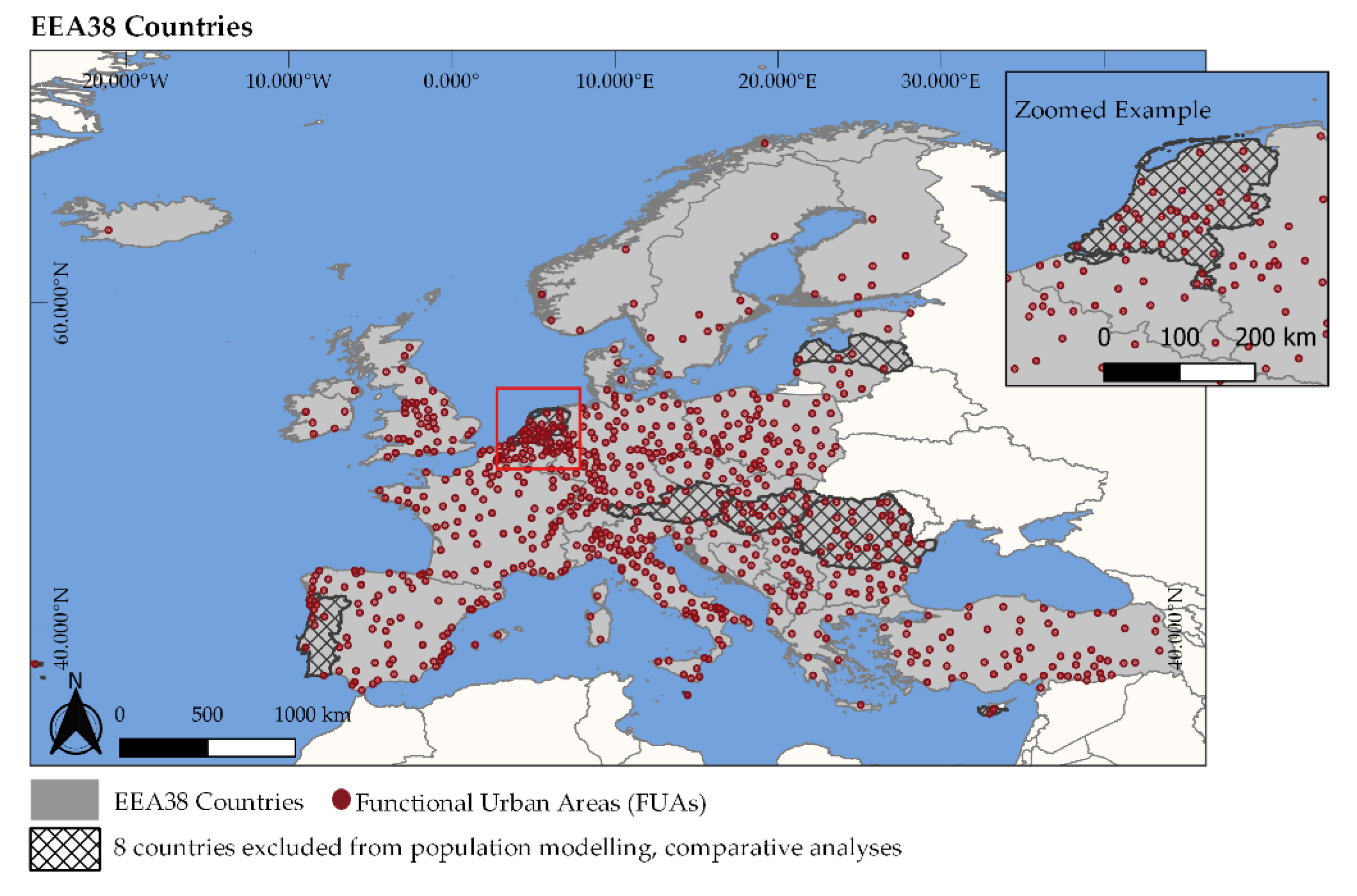
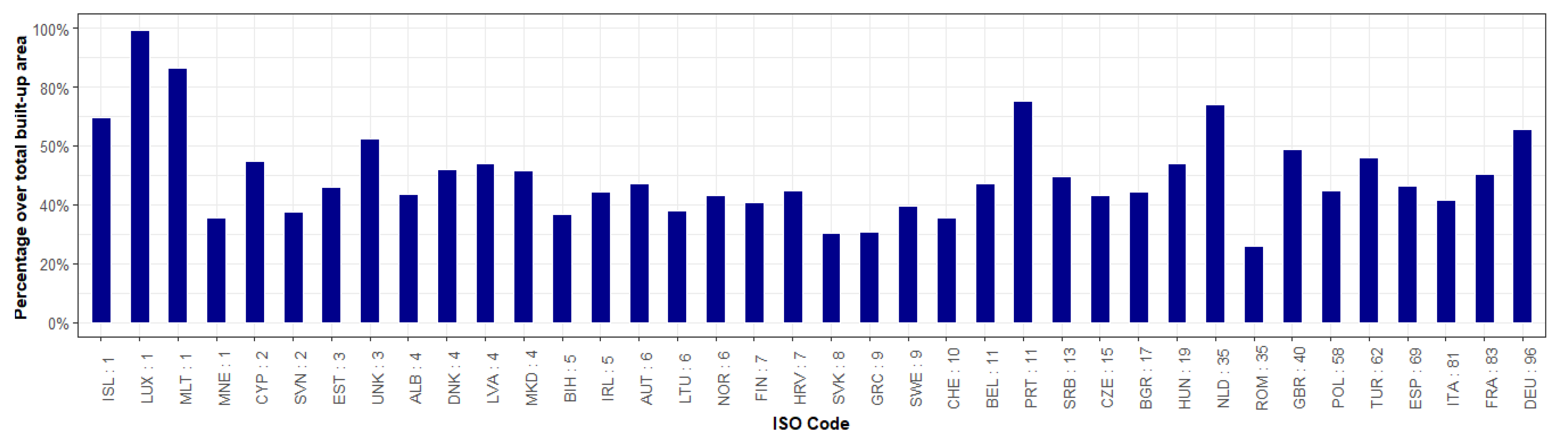
2.1. Study Area

The study area of our analyses covered the 38 countries in the European Union Area (EEA), including the member state countries of the European Union (EU), the countries of the European Free Trade Association (EFTA), the West Balkans countries, Turkey and the United Kingdom, as illustrated in Figure 1.
The selection of this study area was primarily guided by the parallel availability of standardized land-use data from the Urban Atlas dataset (see Section 2.3 for more details) and contemporary high-resolution population data needed for model training, population modelling and validation. In addition, the unique characteristics of each country in terms of the 3D morphology and functional use of the built-up environment, provided with an excellent set up in which to test whether the contributions of the WSF3D dataset in the field of large-scale population modelling were systematically consistent across variable landscapes.
On the one hand, binary classification maps differentiating industrial and non-industrial built-up settlements (Section 2.5) were produced for the EEA38 countries using training, tests and validation datasets collected from a number of Functional Urban Areas (FUAs) (Section 2.3) spread across all countries (red points). Tasks related to population modelling and comparative analyses in population estimates (Section 2.6), on the other hand, were carried out only in 30 countries, excluding Austria, Cyprus, Hungary, Latvia, Malta, Netherlands, Portugal and Romania (crossed-out polygons) where no open population data were available (Section 2.4).

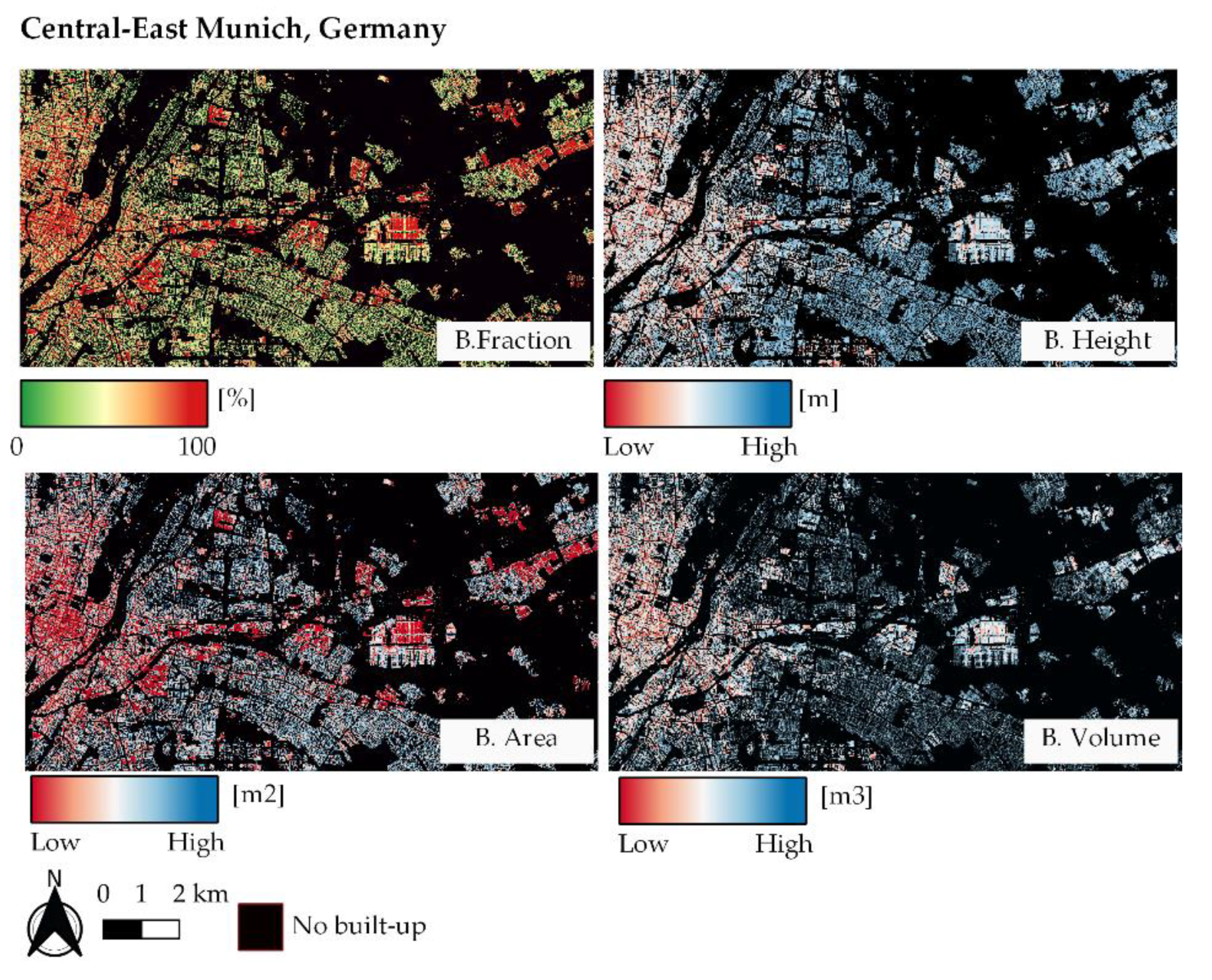
2.2. World Settlement Footprint 3D Dataset

The WSF3D dataset is part of the WSF project and service portfolio developed by the German Aerospace Center (DLR). This dataset includes a collection of thematic layers quantifying the built-up fraction (BF), average building height (BH), total built-up height (AH) and total built-up volume (BV) within a 90 m cell, based on a 12 m building mask (BM). The processing methodology of the WSF3D dataset is based on the work presented by Esch et al. [59]. Concisely, the production approach of the WSF3D relies on two main input datasets: (1) the 12 m spatial resolution TanDEM-X Digital Elevation Model (TDX-DEM), including its underlying amplitude imagery (TDX-AMP), and (2) an updated version of the WSF imperviousness (WSF-Imp) dataset depicting the percent of impervious surface (PIS) at ~10 m spatial resolution [34,60] within the built-up area defined by the World Settlement Footprint 2019 (WSF2019) human settlement mask [61].
For each of the EEA38 countries, the layers employed for this research were provided ready-to-use by DLR. Here, we include a short description of the production process of each layer, focusing specifically on the 12 m versions displayed in Figure 2:
  • Building Height (BH): The 12 m BH layer represents a spatial disaggregation of the standard 90 m WSF3D BH layer, which was derived by measuring the height variations of vertical edges related to building edges (BE) in the 12 m TDX-DEM within the settlement areas defined by the WSF-Imp layer. The height is reported in meters (m) in the final product.
  • Building Fraction (BF): This layer was produced by quantifying the built-up coverage at 12 m derived from the joint analysis of the WSF-Imp, TDX-AMP and BE. The values in the final product range from 0–100, measured in percentage.
  • Building Area (BA): This layer was derived by multiplying the BF times the area of each ~12 m grid cell (~144 m2 at the equator). The area is reported in square meters (m2) in the final product.
  • Building Volume (BV): This layer was derived by multiplying the BH with the area of the 12 m pixels. The total volume is expressed in cubic meters (m3) in the final product.
  • Building Mask (BM): This layer represents the binary version of the BF layer, where all pixels PIS > 0 have been converted to values of 1.
Figure 2. World Settlement Footprint 3D. From top left to bottom right: building fraction (BF), building height (BH), building Area (BA) and building Volume (BV) covering the area of central-east Munich in Germany.
Remotesensing 14 00325 g002

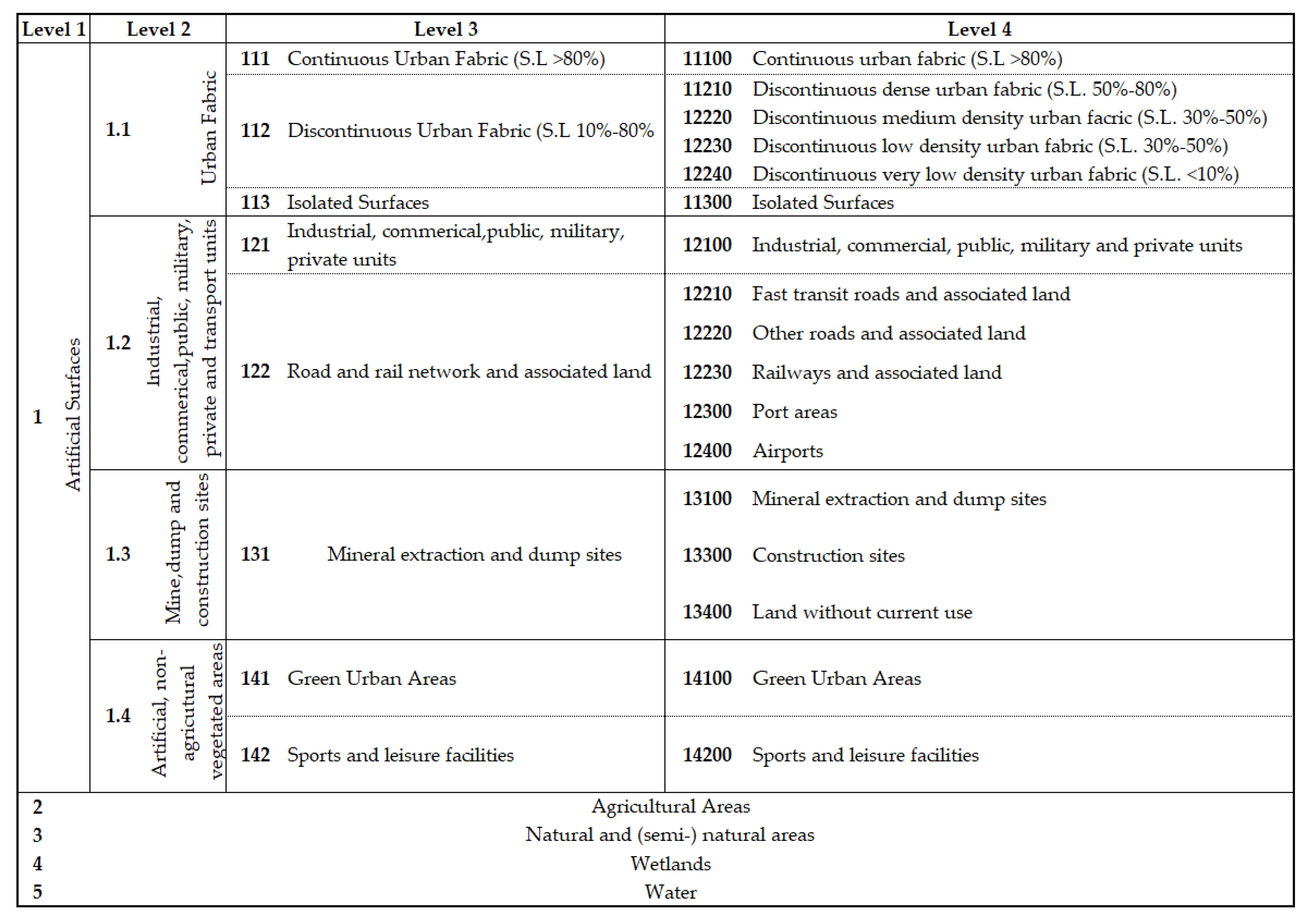
2.3. European Urban Atlas Datazset

The European Urban Atlas is a dataset produced and supported by the European Space Agency (ESA) and the European Environment Agency (EEA). It provides standardized vector land-use and land-cover (LU/LC) data covering more than 700 Functional Urban Areas (FUAs) and their immediate rural vicinity, with more than 50,000 inhabitants across the EEA38 countries. The cartography of the Urban Atlas polygons is based on image interpretation of very high-resolution satellite data (2 m or 4 m spatial resolution). The LU/LC nomenclature is composed of 27 classes distributed in five major groups (Level 1) as described in Figure 3. Within each FUA, LU/LC polygons have a minimum mapping size of 0.25 ha for classes with class code 1, and 1 ha for classes with class code 2 to 5, which are spatially distributed in heterogenous patterns [62].
For each country in our study area, the 2018 versions of 13 datasets were downloaded from the Copernicus land monitoring services website [63]. Accordingly, for each country, Table 1 summarizes the number of FUAs employed in this research.

2.4. Population Data and Administrative Boundaries for 2020

The Center of International Earth Science Information Network (CIESIN) provided upon request the subnational administrative boundaries and the corresponding 2020 census/estimate-based population data for 30 of the EEA38 countries in our study area. According to the technical description presented in [64], the geographical boundaries and population counts follow the cartography and official estimates collected in the 2010 round of Population and Housing Censuses, that took place between 2005 and 2014. For each subnational boundary two types of population data estimates were provided: (i) census/estimated-based numbers calculated using annual exponential growth rates, and (ii) United Nation-adjusted estimates [65], which were used in this research.
Table 2 shows a summary of the population data for each country including the ISO-code, base census year, total population estimation and number of administrative/spatial units. For the purpose of this research, two levels of aggregation of the administrative units were provided: one used for population modelling which was the administrative level 0 or national polygon for each country (hereinafter referred to as L0-units), and one for used for validation which included the finest administrative levels available for each country (hereinafter referred to as L1-units).

2.5. Industrial and Non-Industrial Classification of Built-Up Settlements Using Random Forest

In the field of land-use mapping, research has shown that spatial metrics derived from remotely sensed data combined with a Random Forest (RF) algorithm can be used to effectively to identify different land-use/land-cover classes on the ground [52,66,67,68]. On the one hand, spatial metrics quantitatively describe the configuration of the landscape in terms of the structure (e.g., shape, size, number, density) and the arrangement of elements (e.g., buildings) across space [69]. At a specific scale and resolution, differences in these metrics are normally an indicator of different land-use classes, thus allowing the production of LU/LC classification maps. In the framework of this research, for example, previous studies have shown that spatial metrics such as the average, median and standard deviation of the density, height and volume of building structures can be used to discriminate industrial (and large commercial) buildings from residential and other non-industrial buildings [55]. Overall, industrial buildings are generally larger, higher and denser in comparison with residential buildings, allowing their identification through different remote sensing techniques.
The RF classifier, on the other hand, is a robust ensemble machine algorithm that has proven to be a powerful tool capable to perform accurate supervised classification tasks [70]. Essentially, the RF classifier builds multiple decision trees, each one constructed using a random subset of the training data. Each individual tree delivers a class prediction, and the class with most votes becomes the model’s prediction. Compared to other classification algorithms which are also known to produce robust classifications in remote sensing problems (e.g., support vector machines SVM), the RF performs equally, with the advantage that is easier to implement as it requires less parametrization [71].
Following these premises, in this research we combined an RF classifier with a set of spatial metrics derived solely from the WSF3D layers to predict the “industrial” versus “non-industrial” class of the built-up settlement pixels in each country of our study area. The whole workflow for the production and validation of the final binary classification maps is shown in Figure 4, followed by a detailed description of the main steps in the following sub-sections. Unless indicated otherwise, all processing steps were carried out using GDAL-commands in a Linux environment and Python programming language and libraries.

2.5.1. Derivation of Spatial Metrics

In this study, a total of 16 spatial metrics derived from the WSF3D dataset were used as variables to train the RF models for each country. These included the four basic components of the WSF3D dataset: BA, BH, BF and BV, and 12 additional metrics based on distributional statistics calculated over a 25 × 25 window size (300 × 300 m): mean, median, and the standard deviation. The window size was chosen to ensure that the surroundings of the potentially smallest “non-industrial” areas were evaluated, using as reference the minimum size employed in the cartography of the Urban Atlas datasets (1 ha, 100 × 100 m) [72]. For each country, a 16-band raster composite was generated, which included the total of all parameters derived.

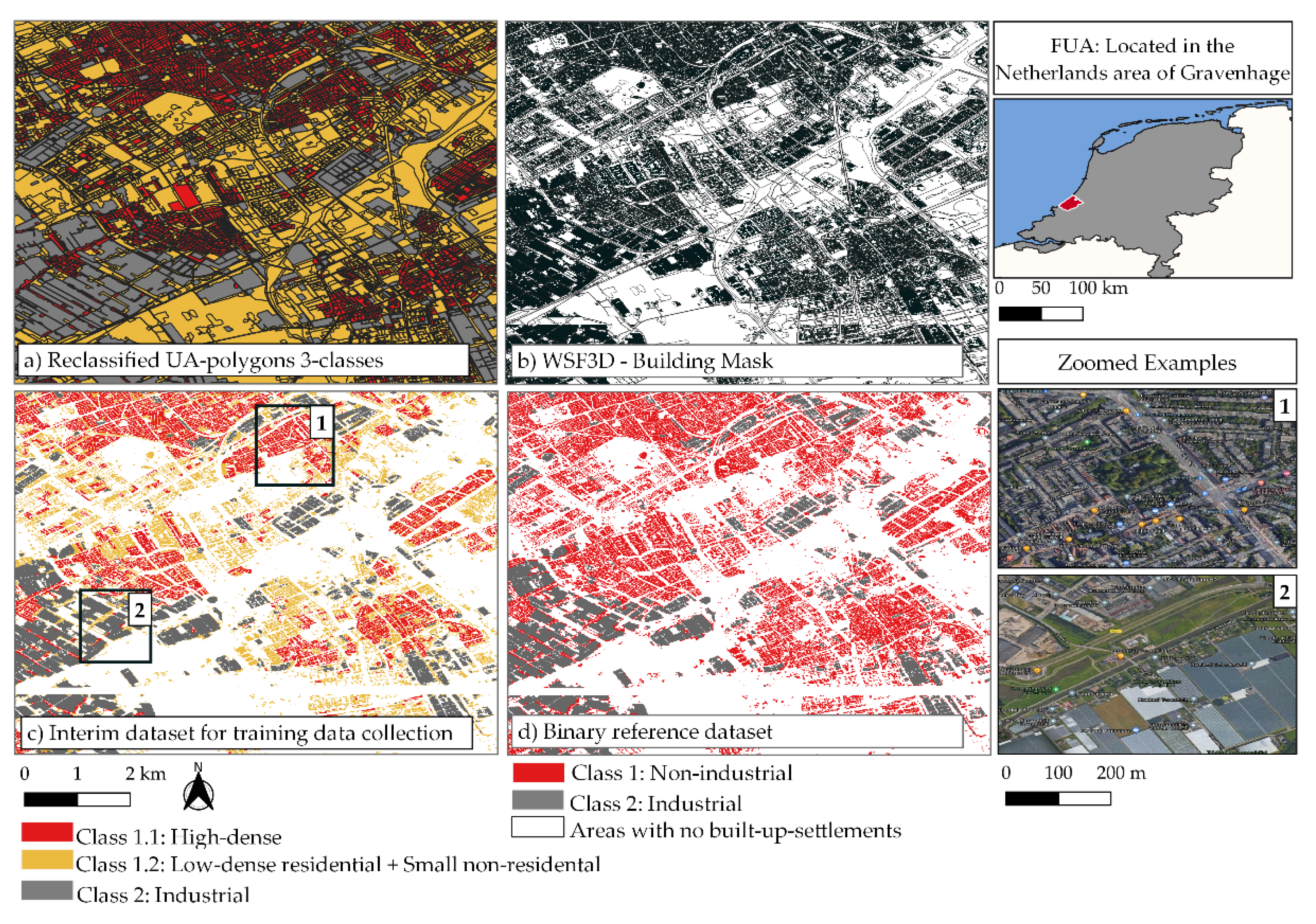
2.5.2. Interim and Reference Datasets

Following methodologies similar to the ones presented in [73,74], interim and reference datasets needed to automatically collect training and test data, and to validate the final classified maps, were produced using the Urban Atlas datasets. For each country the interim and reference datasets were produced by classifying the built-up pixels of the WSF3D building mask (BM) layer according to the class of the Urban Atlas polygons their centroid fell into. As seen in Figure 5, the final interim/reference datasets covered a little more than 50% of the total built-up area for six countries, between 40 and 50% for 24 countries, and between 25% and 35% for eight countries.
Using the reclassification scheme presented in Table 3, for each FUA, built-up pixels were classified as “non-industrial” (Class 1) if their centroids were within those UA polygons with Level 2 codes: 111, 112, 113, 121, 122, 131, 141 and Level 1 codes: 2, 3, 4 and 5, respectively (see Figure 3). On the one hand, according to the Urban Atlas-Mapping Guide [72], polygons within the classes 111, 112 and 113 encompass built-up structures that have a predominant residential component, with the occasional presence of mix-use buildings. Polygons within the remaining classes, on the other hand, encompass built-up structures that have industrial, commercial, public and military use, or small built-up structures with non-residential use located in the proximity of roads and train stations, or within construction sites, gardens, zoos, parks or marinas.
As such, in the particular case of class 121, to exclude polygons representing large industrial and commercial units (e.g., energy plants, production sites, retail parks) only polygons with areas below 10 km2 were considered as “non-industrial”. This threshold was selected after a visual assessment of more than 50% of the Urban Atlas polygons across all FUAs, using very high-resolution (VHR) VHR optical imagery. Consequently, all built-up pixels whose centroids were within Urban Atlas polygons with class code 121 and areas >10 km2 were classified as “industrial” (Class 2), including those located within class code 122 polygons, corresponding to ports and airports.
At the same time, for the purpose of training data collection (Section 2.5.3), the built-up pixels within the “non-industrial” class were further differentiated into two sub-classes, namely “High-dense residential” (Class 1.1) and “Low-dense residential + Small non-residential” (Class 1.2) as noted in Table 3 and Figure 6a–c. This sub-categorization was simply carried out to ensure that enough samples were collected within areas where built-up structures could potentially present similar metrics to the “industrial” class, such as the case of high-rise buildings within the 111 class.

2.5.3. Automatic Training Data Collection

Once the interim reference datasets for each FUA within a country were produced, these were used to automatically collect point training data by means of a proportionally allocated stratified random design. From each class (Figure 6c), we collected 1000 samples (or class labels), which resulted in a total of 3000-point samples per FUA per country. The location of these samples was then used to extract the 16 spatial metrics from each country’s 16-band composite, to finally construct the input training datasets for model training (Section 2.5.4). In this research, the selected sample size represented the maximum size in which the training data for the less represented class, in the less represented FUA, was less or equal to 30% of total available pixels. This means that for each class in each FUA, 70% or more pixels were left as independent test data for model prediction and reference class labels for validation purposes (Section 2.5.5). These ratios are inline to the ones employed in Zhang, Li [54], for a similar assessment.

2.5.4. Model Training

To produce the final binary classification maps of “industrial” versus “non-industrial” classes, for each country, a single RF model (hereinafter referred to as Full Model (FM)-RF) was built using Python’s scikit-learn libraries [75]. As described in Figure 4, for each country a single FM-RF was trained using the entire set of training data collected from all the FUAs belonging to a particular country. Here, it is important to clarify that all of the 16 spatial features derived from the WSF3D were used for model training, without the implementation of feature selection, as internal results (not included here) showed that removing features did not improved model predictions. Accordingly, in order to produce the most robust predictions, during the training process, model hyperparameters were independently optimized for each country, and the final model was used to predict over (1) the entire test data and (2) entire country. Hyperparameter selection was carried out using scikit-learn’s “GridSearchCV” functionalities, to select the number of trees, the maximum depth of a tree, the minimum number of samples required to split an internal node or the minimum number of samples required at a leaf node.

2.5.5. Quantitative Accuracy Assessment

To evaluate the classification accuracy of the FM-RF models, for each country, the predictions made over the test data were compared against the reference data by means of a confusion matrix. For this assessment, built-up pixels predicted as classes 1.1. and 1.2 were first merged into a single class, representing the final “Non-industrial” class to match the final binary reference datasets (Figure 6d). From here, for a balanced accuracy assessment, an equal number of pixels were randomly selected for each class, equal to the size of the least represented class (excluding training data points). This sample was then used to derive common statistical accuracy metrics including the Overall Accuracy (OA) and Cohen’s kappa coefficient (k), and the Producer’s and User’s Accuracy (PA, UA) for each class, respectively.
However, considering that a proper accuracy assessment can only be performed in the areas where reference data is available (see Figure 5), to provide a general overview of the relative accuracy that can be expected in the country-wise classification maps, we produced two alternative models to (1) analyse the spatial transferability of our RF-models and (2) compare their performance against “optimal” scenarios (Figure 4, dashed process). First, following recent methodological guidelines [76,77,78], for each country, k external models (E-RF, k = no. of FUAs) were trained and optimized by excluding the training data of one FUA at the time. In each iteration, the FUA that was left out was used as a spatially independent test area, and the accuracy of its classified map compared against the reference data. Accordingly, for each FUA an internal model (I-RF) was trained and optimized using only each FUAs’ training data. This model was then applied to the test data of same FUA and the accuracy of the classified map compared against the reference data. The results of the I-RF and E-RM were then aggregated at the country level and compared against the accuracy of the FM-RF.

2.6. Population Modelling and Comparative Analyses

Figure 7 illustrates the workflow followed for the assessment of population models built on the basis of the original building mask (BM), building fraction (BF) and building volume (BV) layers of the WSF3D, and a combination of building volume and industrial settlement use information (exclusion of industrial settlements BV-IS).Accordingly, the main steps included the production of gridded population distribution datasets using top-down dasymetric modelling techniques, followed by a well-established quantitative accuracy assessment. These steps are described in more detailed in the following sub-sections.

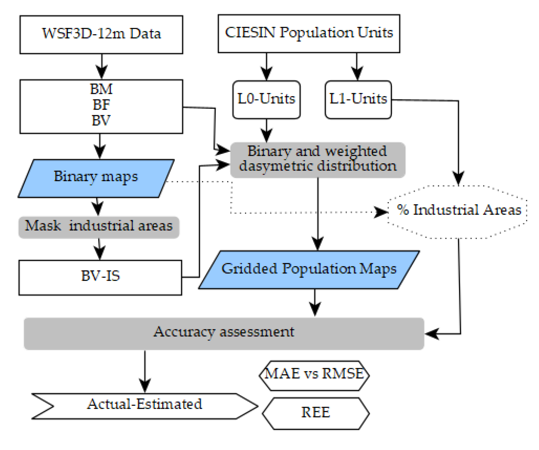
2.6.1. Top-Down Dasymetric Modelling

A total of four gridded population maps for each country were modelled using a dasymetric binary technique or weighted technique, where the 2020 UN-adjusted population counts from L0-units were redistributed into the built-up settlement pixels of the WSF3D datasets. First, gridded population datasets were produced on the basis of the building binary mask (BM) as proxy layer using Equation (1). In this technique, each built-up pixel within a given L0-unit P o p ( p L 0 ) has a weight of one W p = 1 , resulting in each pixel being allocated an equal number of people. This approach is similar to the one employed by the HRSL and the GHS-POP datasets and produces a homogenous distribution of the population within each L0 unit, preserving the original population counts of the input unit.
P o p ( p L 0 ) = P o p L 0 W p p = 1 n ( W p ) { W p = 1 , B M 0 < W p 100 , B F , 0 < W p max ( p v ) , B V , B V I S
Second, gridded population datasets were produced on the basis of the different continuous layers, including the building fraction (BF), building volume (BV) and building volume minus industrial settlements (BV-IS). Here, unlike in the binary technique, each built-up pixel is allocated a proportion of the input unit’s total population P o p L 0 , relative to their density ( 0 < W p 100 ) or volume ( 0 < W p max ( p v ) ) pixel values p v . This approach produces heterogenous population distributions, comparable to the ones provided by the WSF-Pop datasets, preserving the original population counts of the input unit.

2.6.2. Quantitative Accuracy Assessment

As shown by previous studies [9,13,79], in the field of large-scale population modelling, a “true-validation” of gridded population datasets remains a very challenging task due to the lack of high-resolution ground-truth data (e.g., population counts at the pixel level) needed for an independent quantitative assessment. Therefore, in order to test the accuracy of population distribution datasets, the research community has developed an empirical validation method that measures the internal accuracy of population distribution maps in terms of “how well and plausibly populations were distributed” [19].
Overall, in this method a series of statistical analyses are performed using the differences between population counts extracted from maps modelled using a coarser level of the administrative units (here, L0 units or input units), and the population counts of the finest administrative units (here, L1 units or validation units). Here, the main assumption is that input population data is accurate, and as such, the resulting empirical analyses only measure the relative accuracy, effectiveness and stability of the employed disaggregation method and/or proxy layers.
For this research we applied the same validation method to systematically compare the quantitative accuracies of the four different population datasets described in the previous section. First, as explained in Section 2.6.1, we have chosen to model the final gridded population datasets using the national level administrative units for all countries (L0 units). This was carried out to reduce the bias that is normally introduced when the input units and validation units have a similar size [14,80], on the one hand, and to be able to evaluate each country with the largest number of validation units possible (L1 units), on the other [13]. Second, using the L1 units (validation units), from each population dataset we extracted the estimated population counts using the Zonal Statistic tool of ArcGIS. For each country and each gridded population dataset, the reported differences between the actual and estimated values were then used to derive the following error metrics:
M A E c = i L 1 = 1 n | p o p a p o p e | n
% M A E c = M A E c p o p c ¯
R M S E c = i L 1 = 1 n ( | p o p a p o p e | ) 2 n
R E E i L 1 n = p o p a p o p e p o p a 100
On the one hand, for a given country, the Mean Absolute Error (Equation (2)) and Root Mean Square Error (Equation (4)) ( M A E c , R M S E c ) both measure the average of the absolute differences between the actual ( p o p a ) and estimated population ( p o p e ) counts of the L1 units. However, unlike the RMSE, which penalizes larger errors by squaring the differences, the MAE weights each error equally, allowing the identification of outliers in the data. On the other hand, the percentage MAE (Equation (3)), which is the MAE divided by the average population of each country, allows the comparisons across countries by removing the bias of different population totals and number of L1 units. This metric can be used to determine if the errors/improvements generated by the different proxy layers are similar and systematic, or if different behaviors are observable across countries.
The Relative Estimation Error (REE, Equation (4)) measures the error in each L1 unit in proportion to their actual population counts. By reducing the bias caused by differences in population counts across L1 units, this metric is useful in comparing the distribution of errors within countries and across countries produced by each covariate layer. In this research, the REE was used in two ways:
(i)
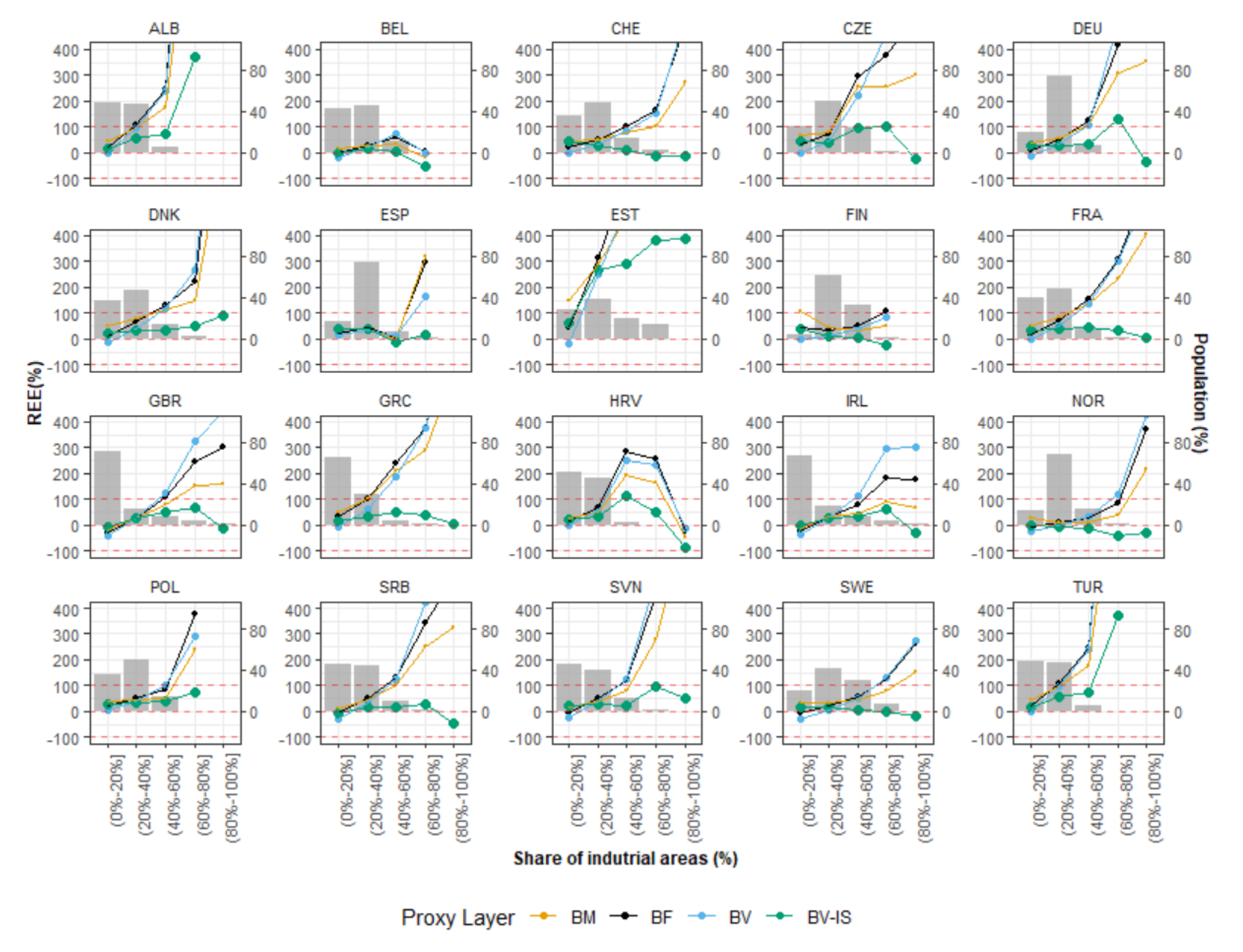
Firstly, for each country we calculated the proportion of industrial areas found within the L1 units according to the final binary classification maps. For all L1 units with the same amount of industrial presence, we then calculated the average REE produced by each gridded population map.
(ii)
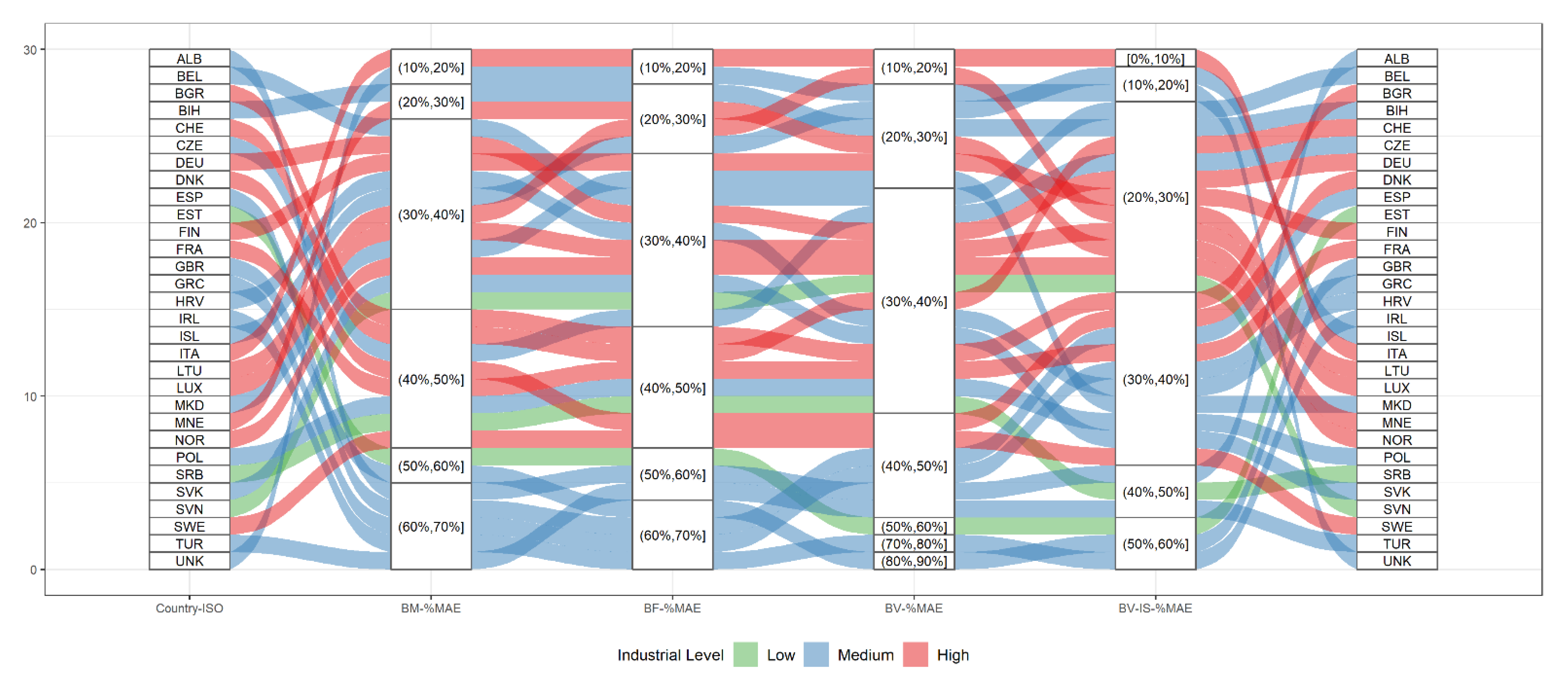
Secondly, similar to [48], we grouped the L1 units into REE ranges of 25% according to the results produced by each gridded population map. For each country, we then calculated the percentage of each countries’ total population found in these units.

3. Results

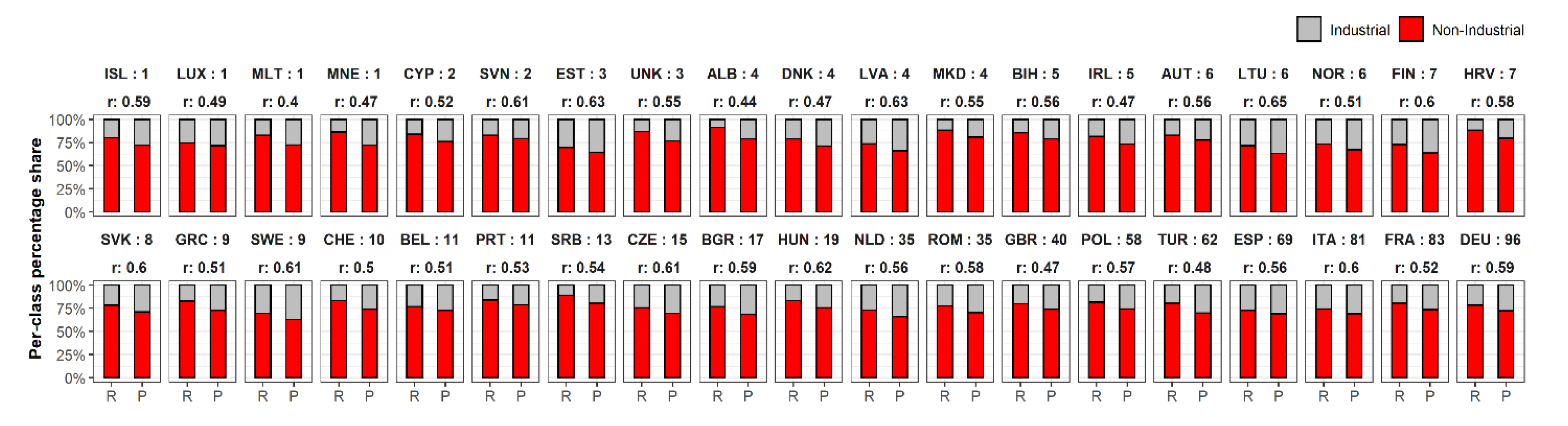
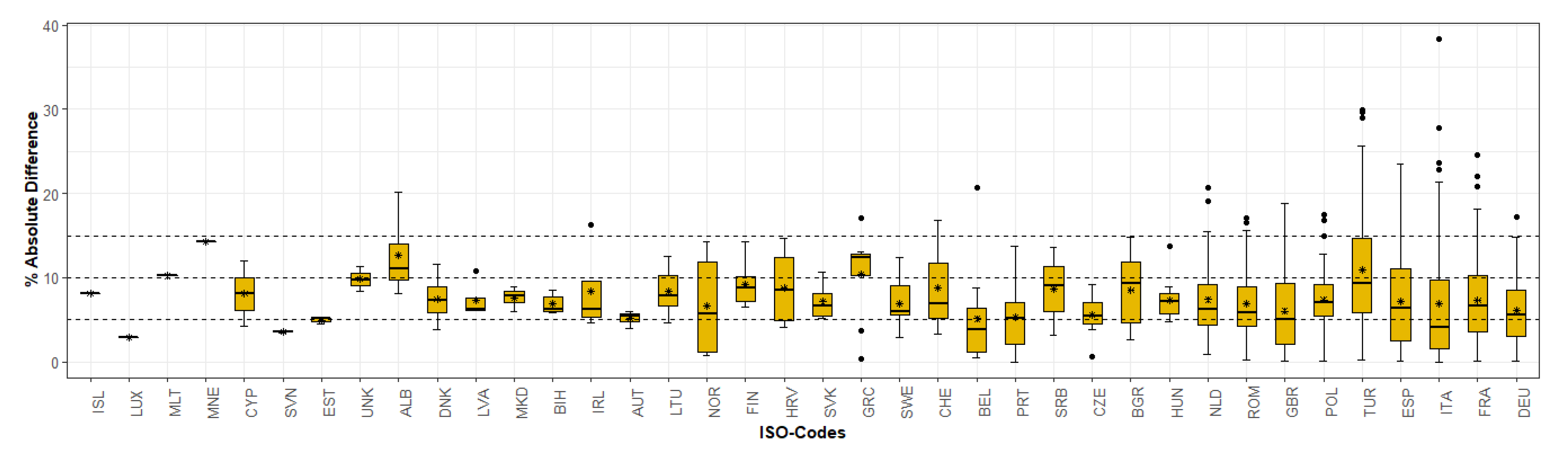
3.1. Industrial and Non-Industrial Binary Classification Maps

To evaluate the overall performance of our automated FM-RF models for the classification of industrial versus non-industrial built-up settlements, Figure 8 together with Figure 9 show the results of comparing the percentage of total area covered by each class according to the reference (R) and the predicted (P) classified maps. First, at the country scale, as seen from the distribution of the per-class percentage share presented in Figure 8, the proportion of built-up settlements pixels predicted as industrial (grey bar) and non-industrial (red bars) types by the FM-RF models were fairly comparable to those reported by the reference maps. As observed, for most countries, there are slight overestimations in the predicted industrial share. Overall, according to the Pearson’s correlation (r) values, the agreement between the reference and predicted maps at the country level ranged from 0.40 (MLT) to 0.65 (LTU), with an average value of 0.54, a median of 0.55 and a standard deviation of ±0.05, reported at the Pan-European scale.
At the FUA level, a closer look at the distribution of the absolute differences in class proportions presented in Figure 9, reveals that for most countries (24/38) at least 75% of the FUAs’ predicted maps (IQR range box) showed differences in class proportions below 10% compared to their respective reference maps. For the remaining 25% of the maps, and for 9 of the 14 left countries, differences did not exceed 15%. As such, differences in class proportions between the predicted and reference maps equal or larger than 20% (but lower than 40%) were only found in a small number of outlier FUAs in BEL, NDL, TUR, ITA and FRA.
To complement the aforementioned results, Figure 10 shows the accuracy metrics reported by the confusion matrix analysis, for the FM-RF (black), the I-RF (red) and the E-RF (blue) models, respectively. Focusing first on the results produced by the FM-RF, results show that in terms of the overall accuracy (OA), for most countries, the accuracies were higher than 85%. The highest value of 90% was reported in LTU, whereas the lowest value of 75% was reported in MLT. Overall, at the Pan-European scale, the OA reported by the FM-RF reached an average of 84.32%.
Accordingly, for most countries (22/38), the Cohen’s kappa coefficient (k) values remained higher than 0.7, with the highest value of ~0.82 reported in LTU. Fifteen out of the remaining sixteen countries reported k-values higher or close to 0.6, with the lowest value of ~0.52 reported in MLT. At the Pan-European scale, the k value reported by the FM-RF reached an average of 0.68.
In terms of the Producer’s Accuracy (PA) for class 1: non-industrial and class 2: industrial, results reveal that in 37 of the 38 countries, the PA of class 1 was close or higher than 90%, with the lowest metrics of 85% reported in MLT and the highest value of ~95% reported in ISL, SVN, NOR, HRV, GRC and HUN, respectively. Conversely, the PA of class 2 was higher or equal to 80% for 23 countries and between 70% and 80% for the rest of the countries. The highest value of ~87% was reported in LTU and the lowest value of ~72% was reported in MLT and GBR, respectively. Overall, at the Pan-European scale the PA of the non-industrial and industrial classes, reached an average of 92% and 79%, respectively. Accordingly, results reveal than in 21 of the 38 countries, the User’s Accuracy (UA) of class 1 was higher or equal to 80%, between 70% and 80% for nine countries, and below 70% for eight countries. The highest value of ~87% was reported in LTU, and the lowest value of ~65% was reported in MLT and GBR, respectively. Conversely, the UA of class 2 was higher, equal or close to 90% for 36 of the 38 countries. The highest value of 95% was reported in HRV, and SVK, and the lowest value of ~82% was reported in MLT, respectively. Overall, at the Pan-European scale, the UA of the non-industrial and industrial classes, reached averages of 76% and 91%, respectively.
Finally, from a comparative point of view, the results produced by the different RF-models reveal that the FM-RF models performed fairly comparable to the I-RF models, while marginally improved over the E-RF models across all countries. As observed, in terms of the OA, the difference between the FM-RF and the I-RF was only 2%, and between the FM-RF and the E-RF only 3% at the Pan-European scale. Accordingly, the kappa coefficient dropped 0.04 between the FM-RF and the I-RF, while it improved 0.02 points between the FM-RF and the E-RF. In terms of the PA and UA the trends are similar, where the largest difference of 4% can be seen between the PA od the I-RF and the FM-RF models.

3.2. Population Modelling: Output Gridded Population Maps

Figure 11 shows several extracts of the output gridded population maps produced using the four proxy layers (BM, BF, BV and BV-IS) and the national level (L0 units) administrative units. Each map was produced at a spatial resolution of 12 m, representing the estimated amount of people per pixel for the year 2020. To visually inspect the thematic differences between maps, we focused on representative areas with a mix of non-industrial and industrial areas, including ports and commercial centers. As observed, gridded population maps produced on the basis of the BM proxy layer delivers homogenous distributions of the population, where each pixel holds the same amount a people. Gridded population maps produced on the basis of the BF, BV and BV-IS, on the other hand, offer more spatial heterogeneity, adhering to the relative changes in the density and volume values, respectively. Without the inclusion of settlement use information, it is possible to observe that maps produced with the BF and BV layers allocate a large proportion of the population in areas identified as Industrial in the BV-IS maps. The BV proxy layer, however, seems to minimize this effect, by allocating a higher proportion of the population in the dense non-industrial areas, as opposed to the BF, where the allocation of people in dense non-industrial areas and industrial areas appears balanced.

3.3. Population Modelling: Quantitative Comparative Analyses

The results of the accuracy assessment for each of the gridded population dataset in terms of the %MAE are presented in Table 4. Overall, results indicate that the integration of volume and industrial settlement use information (BV-IS) produced the lowest %MAE errors in the majority of the countries (bold numbers), whereas the BM produced the highest %MAE (italic numbers), respectively. At the Pan-European scale, 75% of the countries reported %MAE was equal or below 47.26%, 46.06%, 42.93% and 37.72%, using the BM, BF, BV and BV-IS proxy layers, respectively. Here, the lowest %MAE value reported by each layer was 16.15%, 14.88%, 11.66% and 8.47%, respectively; while the highest %MAE value was 68.37%, 67.25%, 80.13% and 56.92%, respectively.
To evaluate the correlation between industrial coverage and the %MAE reported by each proxy layer at the country scale, we categorized the countries into three industrial levels, namely “Low” (0–10%), “Medium” (10–20%) and “High” (>20%) according to the share of industrial areas found according to the classified maps. With this, we then evaluated %MAE that was reported by each country’s population map transitioning from one proxy layer to the next (BM to BF, BF to BV and BV to BV-IS) as described in Figure 12.
As observed, results indicate that only two out the 30 evaluated countries fall within the “Low” category of industrialized level, whereas 15 and 13 countries fall within the “Medium” and “High” category (see Table 4), respectively. For countries with “Low” industrial coverage, the %MAE remained some-what stable from one proxy layer to the next, where improvements of 10% are only reported in SVN by the BV-IS proxy layer. For countries with “Medium” and “High” coverage this behavior is a more variable. First, independently of the error range, for most countries (22/28) the %MAE produced by the BM proxy layer remained within the same range as %MAE produced by the BF proxy layer. Here, six countries reported improvements of 10% (4 “Medium”, 2 “High”), while one country (GBR) reported 10% worsening. Consequently, for 12/28 countries errors remained within the same range between the BF and BV proxy layers. Here, 12/28 reported improvements (7 “Medium”, 4 “High”), elven countries of 10% and one country (GRC) of 20%. Three countries reported worsening of 10% and one country of 20% (GBR). When transitioning from the BV to the BV-SI, for 11/28 the %MAE remained within the same error range: Here, 14/28 countries reported improvements (7 “Medium”, 7 “High”), twelve of 10%, one of 20% (IRL) and one of 30% (GBR). Three countries reported 10% worsening. Finally, a general evaluation transitioning from the BM to the BV-IS shows that 9/30 countries remained within the same %MAE errors range, from with one had “Low” industrial coverage, seven “Medium” industrial coverage and 1 “High” industrial coverage. Therefore, 21/30 countries show improvements, 15 of 10% (1 “Low”, 4 “Medium”, an” 10 “High”), 5 of 20% (3 “Medium” and 2 “High”) and one country of 30% (“Medium”).
In terms of the MAE and the RMSE, the results in Figure 13 show that for most countries and proxy layers, the MAE value remained at least twice as low as the average population at the country level. This behaviour was not similar for the RMSE, where for most countries this value was higher than the average population with the BM, BF, BV and BV-IS proxy layers, respectively. Accordingly, within most countries the distance between these two metrics is relatively shorter for models produced with the BV and BV-IS layers, respectively. This means, that in models produced with the BM and the BF layer, a larger variability exists between errors, which also suggest the presence of one or multiple outliers.
As described in Section 2.6.2, to compare the general trends of error distribution delivered by each proxy layer, we investigated the relationship among the Relative Estimation Error (REE), the total population and the share of industrial areas found within the validation L1-units of each country. Figure 14 presents the results of this assessment, where we have included only those countries where the majority of industrial ranges were present, with the rest of countries showing similar trends.
First, as seen from these plots, the largest proportion of each countries’ the population (bar plots, y-right-axis), is mainly found in units where the calculated industrial presence is below 40%. As the share of industrial areas increases, the average population decreases, reaching values equal or below 20% for most countries. Second, by analyzing the distribution of the REE (line/point y-left-axis), one of the general trends we can observe, is that the majority of the proxy layers produced errors of overestimation across all ranges of industrial share (points above the “0” horizontal line). Errors of underestimations, produced mainly by the BV (light blue) and BV-IS (green) proxy layers, can be seen in some countries, especially in validation units with an industrial share lower than 20%, and in some few cases in ranges higher than 80%. Accordingly, for the majority of the countries, the BV-IS proxy layer produced overall the lowest REE. While for most countries, this tendency started from validation units with industrial share larger than 20%, improvements over the BM (yellow), BF (black) and the BV (light blue) proxy layers became more pronounced in units with industrial share >40%. For the BM, BF and BV proxy layer, the largest (visible) overestimations are present in units with more than 60% of industrial share. In these units, the BV-IS proxy layer reduces the overestimations by as much as 700%, reaching either overestimations or underestimation in the range of 25–50%.
This behaviour, however, is different in units with industrial shares lower than 20%. For most of the countries, the BV proxy layer produced the smallest errors (underestimation) in the range of 10–15%, followed by BF and BM proxy layers, respectively. Finally, while the REE increased with increasing values of the industrial share for the BM, BF and BV layer, the errors reported by the BV-IS were consistently more stable, remaining systematically between −50% and 100% error ranges, in comparison with the other proxy layers, were errors reached overestimation higher than 400%.
Finally, to evaluate the distribution of error across all countries, Figure 15 shows the share of total population that fell within different REE ranges according to each proxy layer summarized at the Pan-European scale. At this level of evaluation, it is possible to observe that the BV-IS proxy layer estimates close to half of the population with errors ranging from −25% to 25%, with most errors being of underestimation. Comparably, within the same ranges, the BM, BF and BV proxy layers (inner to outer donuts) estimate 37%, 40% and 47% of the population, respectively, also with a tendency to underestimate.
Accordingly, with the BV-IS the second largest proportion of the population (~30%) was estimated with errors ranging from ± (25% to 50%), ~11% was estimated with errors ranging from ± (50% to 75%), ~3% was estimated with errors ranging from ± (75% to 100%), and ~3% with errors >100%. For the BM proxy layer, ~32% of the population was estimated with errors ranging from ± (25% to 50%), ~20% was estimated with errors ranging from ± (50% to 75%), ~7% was estimated with errors ranging from ± (75% to 100%), and ~5% with errors >100%. For the BF proxy layer, ~30% of the population was estimated with errors ranging from ± (25% to 50%), ~20% was estimated with errors ranging from ± (50% to 75%), ~6% was estimated with errors ranging from ± (75% to 100%), and ~5% with errors >100%. Finally, for the BV proxy layer, ~32% of the population was estimated with errors ranging from ± (25% to 50%), ~13% was estimated with errors ranging from ± (50% to 75%), ~5% was estimated with errors ranging from ± (75% to 100%), and ~4% with errors >100%.

4. Discussion

4.1. Industrial and Non-Industrial Classification of Built-Up Settlements Using Random Forest

The results of the classification tasks reveal that spatial metrics derived solely from the WSF3D dataset in combination with an RF classifier can be used to effectively identify and discriminate industrial versus non-industrial settlement use over large territorial extents. First, according to the results presented in Figure 8 and Figure 9, for most countries, the binary maps produced on the basis of the FM-RM models showed good agreement with the reference datasets in terms of the share of built-up settlements belonging to one or the other class. According to the standard interpretation of the Pearson’s’ correlation metric in the context of intraclass correlation [81], the agreement between the refence and predicted maps was- between “fair” (0.4–0.59) and “good” (0.6–0.74) for all countries, highlighting the overall robustness of the presented approach.
Furthermore, as seen from Figure 10, the FM-RF models for most countries delivered average Overall Accuracy (OA) and Kappa coefficient (k) metrics that, at the Pan-European scale, remained above 84% and 0.68, together with Producer’s Accuracy (PA) and User’s Accuracy (UA) metrics that remained above 92–79% and 76–91% for each class, respectively. As observed, these metrics were not only fairly comparable to those reported by the I-RF models which, in the framework of our analyses, can be as “the best case scenario” [78], but they also showed high correlation with the metrics of the E-RF models demonstrating that (1) the spatial metrics that characterized the training data for each class were heterogenous for most FUAs, and (2) that that these spatial metrics were similar across FUAs, allowing for the spatial transferability of our approach [82].
In this context, from a comparative point of view, it is also worth noting that the results presented here are in line with those reported in other fine-scale studies that have employed an RF classifier in combination with more accurate and VHR remotely sensed data. For example, for an assessment of the classification accuracy of residential and industrial areas in Yangtze River Delta, China, the authors of [55] reported an OA of 87% and k of 0.74 from RF-models trained using spatial lacunarity metrics derived from VHR-LiDAR data. In the same way, using feature spatial metrics derived from VHR-LiDAR data, building footprints, VHR ortho-imagery (HRO) and Google Street View (GSV) images (GSV), the authors of [54] obtained and OA of 51.4% for commercial and industrial buildings, focusing on two small districts in Brooklyn, New York. Comparably, using spatial metrics derived from VHR ortho-imagery (0.5 m) and OSM parcel data, the authors of [67] reported average OA of ~81.5% for the non-residential class (incl. administrative and commercial services), in Ouagadougou, Burkina Faso and Dakar, Senegal. Here, it is important to note that the WSF3D-based approach presented in our study is globally applicable—in contrast to methods requiring VHR ortho-imagery. Thus, it can be assumed that the approach developed here can easily be applied worldwide and, at the same time, accuracies can be achieved that are in the range of results obtained on the basis of commercial, high-resolution satellite images and building models.
With that being said, while the results presented here illustrate the high potential of the WSF3D dataset for identifying non-industrial versus industrial areas, there were a set of basic components that without a doubt influenced the accuracy of the final binary maps. These can be summarized as follows:
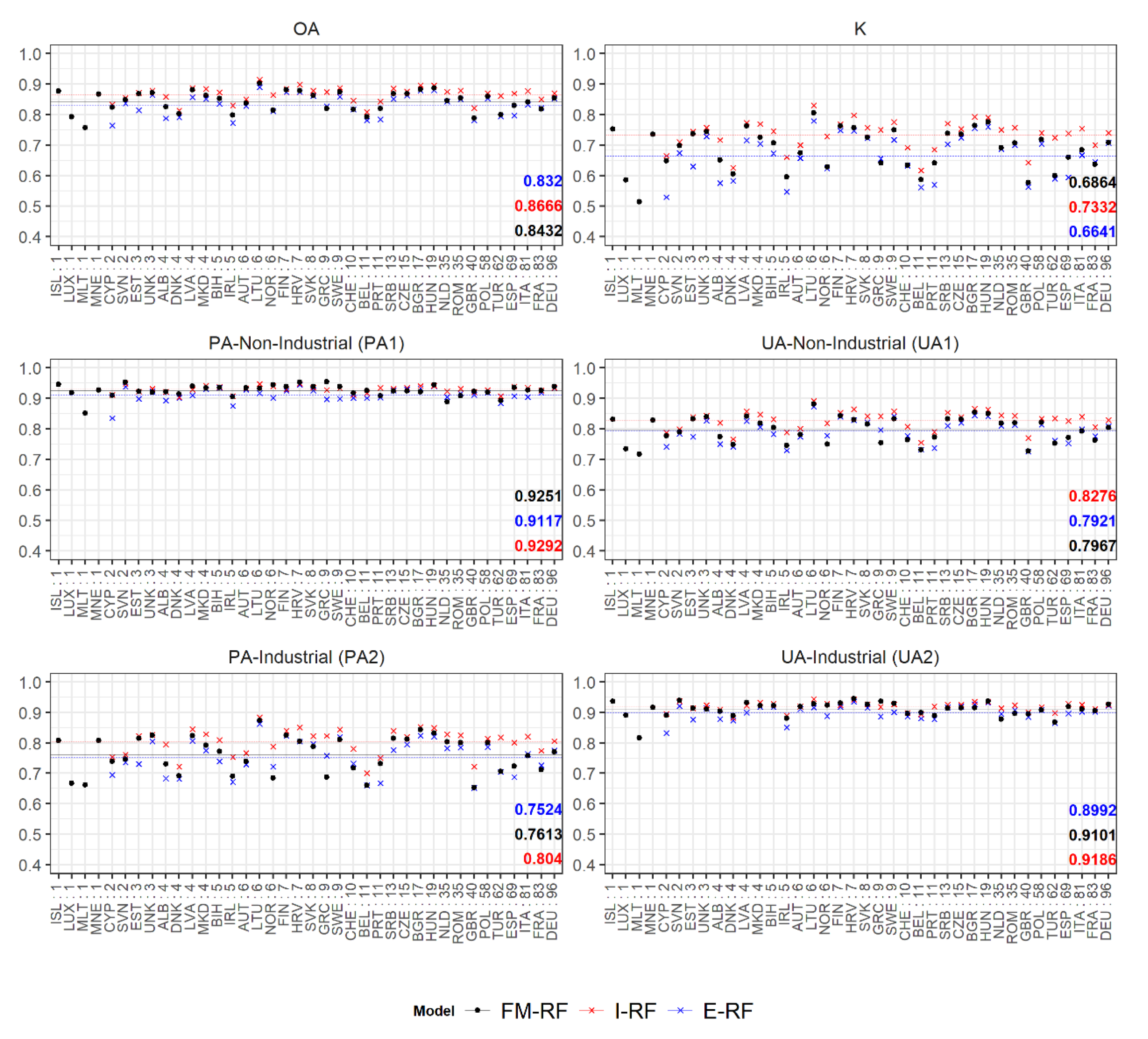
  • WSF3D: The quality and accuracy of the WSF3D in terms of settlement detection (building mask-BM) and the final derived spatial metrics, played a fundamental role in the final accuracies reported in this research. A thorough inspection of the classified maps revealed that in areas identified as “industrial” by the reference datasets, many pixels representing actual green areas or parking lots were detected as built-up in the BM layer. Considering their low spatial metrics, the FM-RF then predicted these pixels as “non-industrial” leading to errors of omission in the industrial class, and errors of commission in the non-industrial class as summarized in Figure 10. In this context, from the average 25% errors of omission reported at the Pan-European level for the industrial class (100–75%, PA2 = 25%), it was found that approximately 15% of the errors came from confusing class 2 for class 1.1, and 10% for class 1.2 (see Table 3) during the prediction process. While the classification of these pixels as “non-industrial” could be in reality “thematically correct”, for the purpose of population modelling the presence of these pixels are detrimental, as population counts are allocated within these areas. Therefore, to potentially reduce the misclassification caused by the false detection of settlement pixels, future research should explore improving the final BM layer by integrating thresholds in the BF layer (Section 2.2). Similarly, the integration of additional post-classification steps should also be considered, such as employing a broader number of window sizes for the extraction of spatial metrics as carried out in [56], or by reclassifying the pixels according to their RF-class probability as carried out in [67].
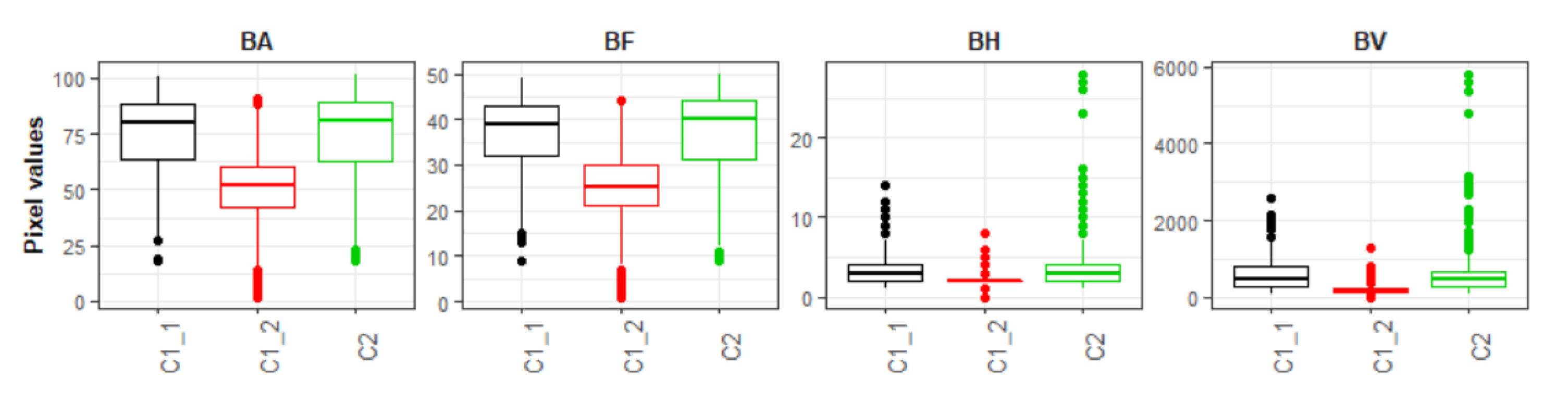
  • Automatic training data collection: Unlike some local-scale research where a manual collection of training samples allows for a visual qualitative assessment of the training data [48], in this research we relied on an automatic procedure that did not include performing any sort of quality control over the training datasets. In correlation with our previous point, in a few cases, this lack of assessment resulted in poorly heterogenous training samples among classes, which without a doubt lead to some misclassification errors. For example, by evaluating the training data of a FUA in Ireland that shows large differences between classes (see Figure 9), it was possible to observe that the pixels values for class 1.1 “High-dense residential” and class 2: “Industrial” were similar across the bands corresponding to the BA, BF, BH and BV as represented in Figure 16. Within the selected FUA, this homogeneity led to errors of omission in the “non-industrial” class close to 20%, which meant that many pixels were erroneously classified as “industrial”. In this framework, while the errors of omission in the non-industrial class at the Pan-European scale are considered low (Figure 10), these misclassification errors had repercussions on the final population datasets, as seen by the results of Figure 14. Therefore, while a manual collection of training samples within the extent of our study area would have translated into a time-consuming task, further research should focus on the implementation of automatic intra-class separability analyses like the one presented in [83], with the objective to produce more significative training datasets.
  • Equal number of training samples per FUA, per class: With the aim of producing robust comparative analyses within a country, in this research, an equal sample size was kept among all FUAs so that the I-RF and E-RF models were trained under similar conditions. In this framework, while the less represented class for some FUAs would reach close to 30% of the total available built-up pixels, in many cases less than 5% of the available pixels per class were used for training. This under-representation, coupled with the limitation mentioned on our previous point, affected the classification accuracy, especially in areas with a high inter-class diversity. In light of this, to improve the classification accuracy, future research should consider the inclusion of additional re-sampling steps. Here, post-classification approaches such as the one presented in [48] could become beneficial, where resampling is carried out using the RF class probabilities to concentrate in areas with high model-uncertainty.
While the aforementioned points refer to the components affecting the accuracy of the final binary maps, there are also a couple of limitations and restrictions that need to be pointed out. On the one hand, while our results suggest that the presented approach has good spatial transferability within countries, it should not be assumed that models trained in one country can successfully be applied to another country. As demonstrated in Figure 10, the E-RF models did not perform better that the FM-RF model, even when the differences were minimal, this indicates that local training data is still preferable to achieve good classification results. In this context, future research should focus on evaluating the spatial transferability across countries, with analyses carried out outside Europe, to include a larger variety of built-up environments.
With that being said, it is then important to recognise that a common limitation of the presented approach, is the impossibility of discriminating small non-residential built-up types such as schools, hospitals, churches, etc. from the WSF3D alone, that in the end affect the final population distributions. This type of function is purely social, and as such, impossible to retrieve from the spatial metrics employed here. In this framework, even when the overall objective of this research was not to generate a land-use maps, we suggest that future work should focus on exploring the synergies between the WSF3D dataset with other remotely sensed datasets, where the inclusion of nightlight-imagery, building footprints and OSM tags/point of interest [57], for example, could result beneficial in the identification and refinement of a more extensive set of land-use classes.
Finally, considering that for this research only an RF classifier was employed, to fully evaluate the suitability of the WSF3D and derived spatial metrics for settlement classification tasks, future research should also explore the implementation of other commonly employed pixel-based classifiers including, but not limited, to K-nearest neighbor and Support Vector Machines (SVM), and compare if higher classification results can be achieved, holding the same degree of automation and spatial transferability.

4.2. Population Modelling

In this research, we produced gridded population datasets across 30 countries located in the EEA area to quantify the improvements in population estimates gained from the inclusion of volume (BV) and settlement use information (BV-IS) derived from the WSF3D dataset. For our assessment, we performed comparisons against other proxy layers, to simulate the thematic characteristics of covariate layers that are currently employed in the production of large-scale gridded population datasets, including the binary approach employed for the GHS-POP and the HRSL datasets (BM), and the density approach employed for the WSF-Pop datasets (BF), respectively.
From many perspectives, the results and conclusions obtained in this research are in line with the results found in other research. The main points can be summarizing as follows:
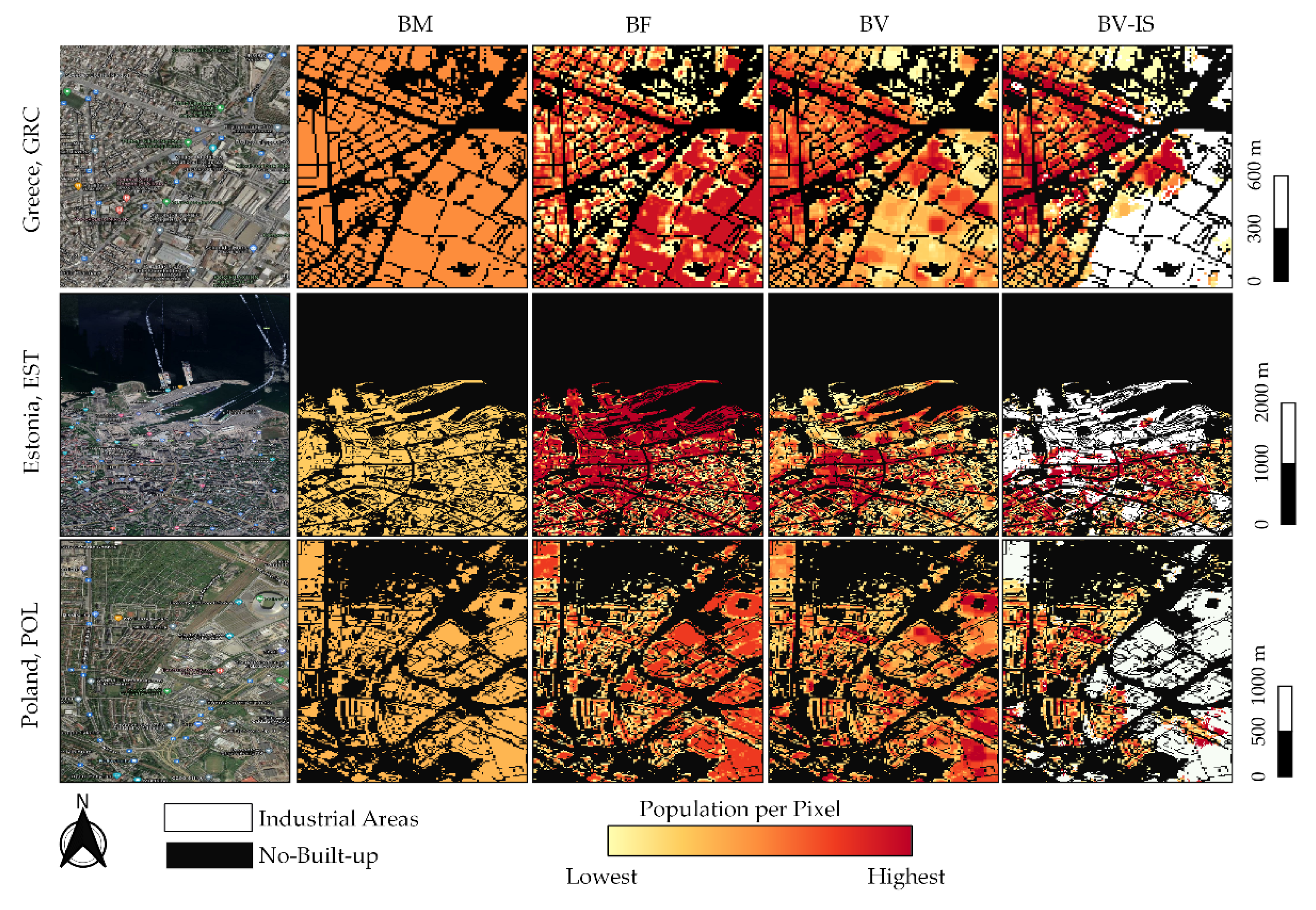
  • Weighted approaches perform better than binary approaches: As already demonstrated in many other studies [13,14,43,44], weighted dasymetric approaches produce higher accuracies than binary dasymetric approaches. First of all, as observed in Figure 11, from a qualitative point of view, the output population maps produced with the “density” layers (BF, BV and BV-IS) show a higher spatial correlation with the underlying rural-urban gradient in comparison to those produced with the binary layer (BM). The results of the quantitative assessment, further confirm that the spatial representations of the population distribution are not only more “realistic”, but also more accurate, as all “density” layers consistently reported better aggregated statistics (%MAE, MAE and RMSE values) compared with the binary layer. On this note, however, it is worth noticing, that at level of validation units (REE), the BM proxy layer is capable to outperform the results of the “density” layers, especially in areas with a large share of industrial areas (see Figure 14). This makes sense if one considers that the “density” layers (BF and BV) amplify the errors of overestimation in these areas, by erroneously allocating more population due to their weighting value.
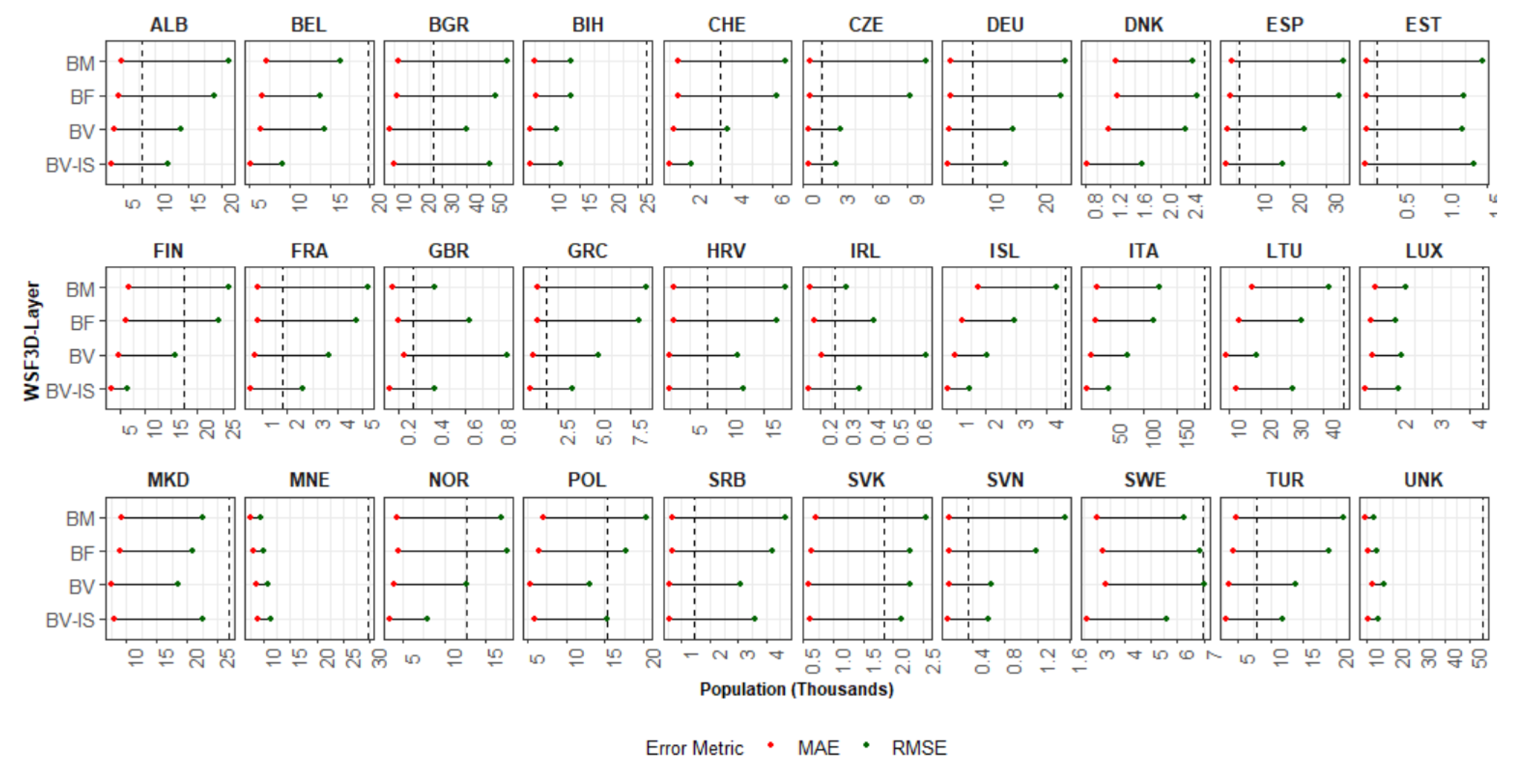
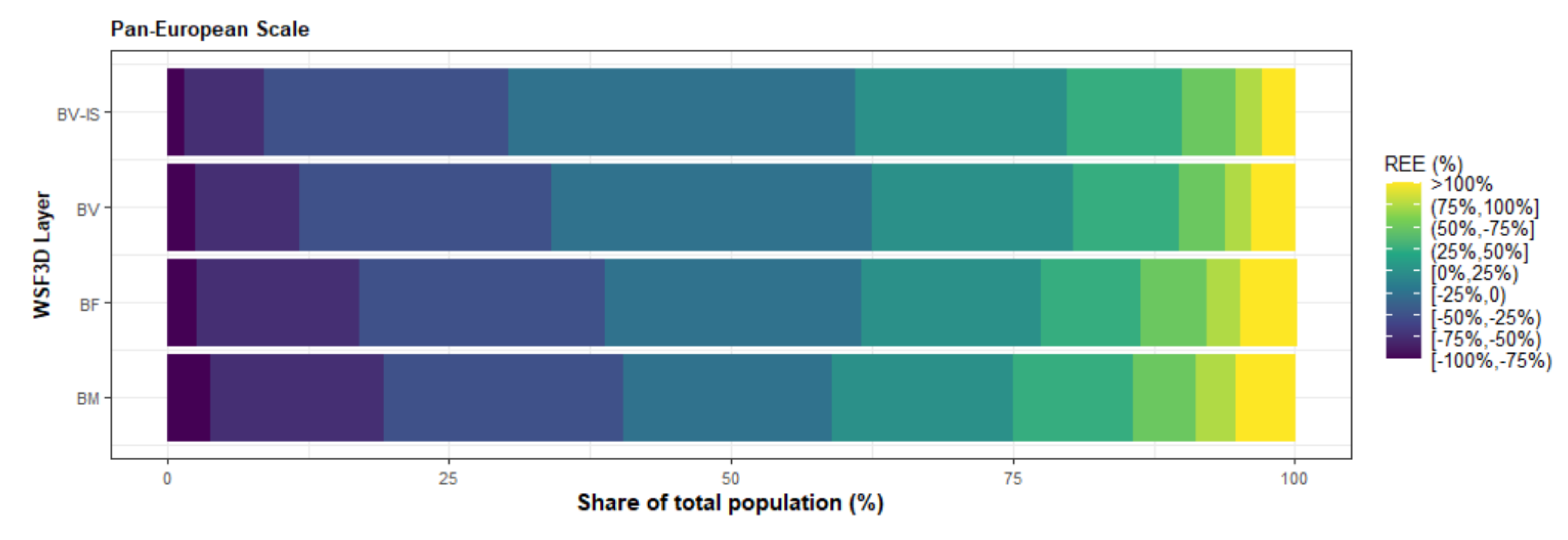
  • Building volume and settlement use information improve population estimates: Comparable to the conclusions reached in local- and national-scale studies [31,48,50], the inclusion of volume and settlement use information derived from the WSF3D dataset produced by far the best estimation accuracies across the majority of the countries. First, according to the results presented in Table 4 and Figure 12, the BV-IS proxy layer produced improvements over the BM, BF and BV proxy layers that reached %MAE values up to 30%. These were more frequently present in countries with “High” industrial coverage, where large errors were remarkably reduced as observed from Figure 14. Second, as observed in Figure 13, the BV-IS proxy layer remarkably reduced the differences between the MAE and RMSE metrics. This was, once again, correlated to the fact that large errors of overestimations were drastically reduced by the proxy layer, especially in areas with a high share of industrial land cover (Figure 14). In this context, the inclusion of settlement use information played a major role, as it allowed the BV-IS proxy layer to produce systematically more stable results across all countries, and across all validation units, while REE errors remained between −50% and 100% with the BV-IS layer for most countries, the BM, BF and BV proxy layers produced variable results that reached overestimations in the rage of 500% or even higher (close to 4500% for EST). Accordingly, at the Pan-European scale, the BV-IS proxy layer estimated a larger proportion of the total population with errors in ±25% in comparison to BM add BF proxy layer, which according to pre-established rankings of accuracy [79], can be considered as “accurately” estimated.
  • The input and validation units influence accuracy results: It is important to note that the maps evaluated in this research have been produced with the coarser administrative population units for each country (national scale). In some countries, where the BV-IS did not report the same systematic improvements compared to the other proxy layer, this characteristic might have influenced the accuracy results. For example, in the case of ALB, EST and TUR (Figure 14), many validation units that reported high coverage in industrial areas still reported large errors of overestimation with the BV-IS layer. This is, because even when industrial areas were successfully identified, the very low population counts of the validation units (sometimes less than 100) were difficult to match from a national-scale disaggregation. In this context, it can be expected for maps produced with the highest level of administrative units to be more accurate than the maps presented here. This assumption is supported by the large amount of research that has already proven that population maps produced with the finest administrative units produces the most accurate population maps [14,31,48,80]. However, considering that this only affected a few countries, also indicates that BV-IS proxy layer is capable to produce more accurate population maps than the rest of the proxy layers, when high-resolution input population data is not available.
  • The relative effectiveness of the BV-IS proxy layer is heavily dependent on the quality of the classified maps: While the BV-IS produced consistently great improvement of the BM and BF proxy layers, in a few cases the performance of the proxy layer was improved by the BM and BV proxy layers, respectively. For example, as observed from Figure 14, in the majority countries the BV proxy layer produced better results than the BV-IS layer in validation units with industrial share below 20% (or 80% non-industrial). In these units, errors of were ~50% higher (mostly overestimations) with the BV-IS layer, which suggest that a number of non-industrial built-up settlements pixels were erroneously removed, causing an allocation of a larger population in the remaining pixels. In this context, as expressed in the previous section, these results correlate to the difficulties of accurately classifying built-up settlements pixels in complex urbans settings, where high-rise buildings are mixed with industrial areas. Here, improvements in the classification process should then reflect in improvements in the population distribution.
With that being said, when evaluating the aforementioned points, a consideration to keep in mind is to recognize that the results presented here are strictly constrained to the employed validation method. The quantitative assessment was conducted following two main assumptions (1) that the population data used for disaggregation were accurate and (2) that WSF3D dataset and its derived layers (BM, BF, BH and BV) were also complete and accurate. Therefore, while discussing the quality of these two main inputs is out of the scope of this research, uncertainties derived from the inherent shortcomings of each input dataset will by default affect the overall accuracy of the final population dataset.
For example, even when the CIESIN census dataset is the most detailed and complete database available at the global scale [65], we can observe that for many countries the last official population data are from more than 10 years ago (Table 2). This means, that potentially, both the population projections and administrative boundaries are outdated, which translate into errors in the final population maps. In this framework, similar to the points presented in the previous section, future research should focus on extending the methods presented here to areas outside Europe. Testing the presented approach in countries where fine resolution population data is not available, such as many countries in Africa [13], would be of great interest, especially in relation to local-scale applications where current gridded population dataset have presented major limitations [25,45].

5. Conclusions

In this research, we explored the contributions that the new World Settlement Footprint-3D (WSF3D) dataset can bring into the field of large-scale top-down population modelling. We performed a series of quantitative analyses that investigated the potential of the dataset from two main perspectives: (1) its ability to discriminate large industrial areas which in the past have been reported as major sources of under- and overestimation in population estimates, and (2) its capabilities to improve population estimates by integrating volume and settlement use information into population modelling frameworks.
To this end, we first proposed a method that relied on spatial metrics derived solely from the WSF3D dataset in combination with a Random Forest classifier to discriminate industrial and non-industrial areas. Here, our results revealed not only that the WSF3D dataset is capable of producing accurate binary classification maps, but that its performance is comparable to other, more spatially granular, VHR remotely sensed datasets that have been used for the same purpose. Foremost, the findings also indicated that the presented method has strong spatial transferability, which means that the dataset poses a viable solution to the existing gap between local- and large-scale analyses.
Accordingly, by integrating the resulting classified maps into frameworks of population modelling, the results were also promising. The results of our quantitative assessment indicate that inclusion of volume and settlement use information (industrial, non-industrial) derived from the WSF3D dataset produced, by far, the best population estimates in comparison to other commonly employed proxy layers. For the most part, the main advantages delivered from the layer include (i) a remarkably, systematic and consistent reduction in errors of overestimation in areas with a high share of industrial areas, (ii) an improved distribution of population estimates in high-density built-up settings and (iii) an increased ability to produce accurate population estimates in the presence of less detailed input census-based population data.
Notwithstanding these promising results, there is however, room for improvement. The results of the classification tasks, for example, can be further enhanced with the integration of post-classification methods and a more careful collection of training data. These improvements will be directly reflected in final population estimations, where misclassification errors proved to be detrimental in highly dense and highly populated built-up settings.
Overall, the results of this study provide a valuable contribution to the field of large-scale population modelling. The methods presented here show strong promise for helping to bridge the gap between fine- and large-scale efforts aimed at improving top-down population distribution models. As shown, the synergies between volume and settlement use information derived solely from the WSF3D dataset provide the basis to create more accurate global population distribution dataset or related updates for arbitrary regions or countries worldwide. In this context, future developments of this work will include the final production and open release of global gridded population dataset, with unprecedented accuracy and spatial resolution.

Author Contributions

Conceptualization, D.P.-L., T.E., M.M. and P.R.; methodology, D.P.-L.; validation, D.P.-L.; formal analysis, D.P.-L.; investigation, D.P.-L.; resources, T.E. and S.D.; data curation, D.P.-L., M.M., K.M., G.Y. and J.Z.; writing—original draft preparation, D.P.-L.; writing—review and editing, D.P.-L., T.E., M.M., K.M., A.S., J.Z., A.J.T. and P.R.; supervision, T.E., A.J.T. and P.R.; funding acquisition, T.E. and S.D. All authors have read and agreed to the published version of the manuscript.

Funding

This work was supported by the EU-funded ACP-EU Natural Disaster Risk Reduction Program, managed by the Global Facility for Disaster Reduction and Recovery of the World Bank (contract nos. 7194331 and 7196541). This work was funded by the German Academic Exchange Service (DAAD) providing the research fellowship to Daniela Palacios Lopez No. 91687956.

Institutional Review Board Statement

Not applicable.

Informed Consent Statement

Not applicable.

Data Availability Statement

The 2020 UN-adjusted population data presented in this research have been provided by CIESIN (contact Kytt MacManus). The WSF3D 12 m and 90 m dataset is not publicly available due to pending data distribution regulations. Open and free provision is foreseen in the following online platforms: https://urban-tep.eu (accessed on 6 December 2021) and https://geoservice.dlr.de (accessed on 6 December 2021).

Acknowledgments

The authors would like to acknowledge the U.S. National Aeronautics and Space Administration (NASA) contract 80GSFC18C0111 for the continued operation of the Socioeconomic Data and Applications Center (SEDAC), which is operated by the Center for International Earth Science Information Network (CIESIN) of Columbia University. Additionally, the authors would like to thank the following research for their insightful support and orientation in the topic of random forest modelling and validation. In alphabetical order: Mariel Christina Dirscherl, Thorsten Hoeser and Aiym Orynbaikyzy.

Conflicts of Interest

The authors declare no conflict of interest. The funders had no role in the design of the study; in the collection, analyses, or interpretation of data; in the writing of the manuscript, or in the decision to publish the results.

References

  1. Ehrlich, D.; Freire, S.; Melchiorri, M.; Kemper, T. Open and Consistent Geospatial Data on Population Density, Built-Up and Settlements to Analyse Human Presence, Societal Impact and Sustainability: A Review of GHSL Applications. Sustainability 2021, 13, 7851. [Google Scholar] [CrossRef]
  2. Ehrlich, D.; Kemper, T.; Pesaresi, M.; Corbane, C. Built-up area and population density: Two Essential Societal Variables to address climate hazard impact. Environ. Sci. Policy 2018, 90, 73–82. [Google Scholar] [CrossRef]
  3. Tuholske, C.; Gaughan, A.; Sorichetta, A.; de Sherbinin, A.; Bucherie, A.; Hultquist, C.; Stevens, F.; Kruczkiewicz, A.; Huyck, C.; Yetman, G. Implications for Tracking SDG Indicator Metrics with Gridded Population Data. Sustainability 2021, 13, 7329. [Google Scholar] [CrossRef]
  4. Huang, B.; Wang, J. Big spatial data for urban and environmental sustainability. Geo-spatial Inf. Sci. 2020, 23, 125–140. [Google Scholar] [CrossRef]
  5. Estoque, R. A Review of the Sustainability Concept and the State of SDG Monitoring Using Remote Sensing. Remote Sens. 2020, 12, 1770. [Google Scholar] [CrossRef]
  6. Avtar, R.; Aggarwal, R.; Kharrazi, A.; Kumar, P.; Kurniawan, T.A. Utilizing geospatial information to implement SDGs and monitor their Progress. Environ. Monit. Assess. 2019, 192, 35. [Google Scholar] [CrossRef] [PubMed]
  7. Kavvada, A.; Metternicht, G.; Kerblat, F.; Mudau, N.; Haldorson, M.; Laldaparsad, S.; Friedl, L.; Held, A.; Chuvieco, E. Towards delivering on the Sustainable Development Goals using Earth observations. Remote Sens. Environ. 2020, 247, 111930. [Google Scholar] [CrossRef]
  8. Doxsey-Whitfield, E.; MacManus, K.; Adamo, S.B.; Pistolesi, L.; Squires, J.; Borkovska, O.; Baptista, S.R. Taking Advantage of the Improved Availability of Census Data: A First Look at the Gridded Population of the World, Version 4. Pap. Appl. Geogr. 2015, 1, 226–234. [Google Scholar] [CrossRef]
  9. Freire, S.; MacManus, K.; Pesaresi, M.; Doxsey-Whitfield, E.; Mills, J. Development of new open and free multi-temporal global population grids at 250 m resolution. In Proceedings of the 19th AGILE Conference on Geographic Information Science, Helsinki, Finland, 14–17 June 2016. [Google Scholar]
  10. Bhaduri, B.; Bright, E.; Coleman, P.; Urban, M.L. LandScan USA: A high-resolution geospatial and temporal modeling approach for population distribution and dynamics. GeoJournal 2007, 69, 103–117. [Google Scholar] [CrossRef]
  11. Dobson, J.E.; Bright, E.A.; Coleman, P.R.; Durfee, R.C.; Worley, B.A. LandScan: A global population database for estimating populations at risk. Photogramm. Eng. Remote Sens. 2000, 66, 849–857. [Google Scholar] [CrossRef]
  12. Stevens, F.R.; Gaughan, A.E.; Linard, C.; Tatem, A.J. Disaggregating Census Data for Population Mapping Using Random Forests with Remotely-Sensed and Ancillary Data. PLoS ONE 2015, 10, e0107042. [Google Scholar] [CrossRef] [PubMed] [Green Version]
  13. Palacios-Lopez, D.; Bachofer, F.; Esch, T.; Marconcini, M.; MacManus, K.; Sorichetta, A.; Zeidler, J.; Dech, S.; Tatem, A.; Reinartz, P. High-Resolution Gridded Population Datasets: Exploring the Capabilities of the World Settlement Footprint 2019 Imperviousness Layer for the African Continent. Remote. Sens. 2021, 13, 1142. [Google Scholar] [CrossRef]
  14. Palacios-Lopez, D.; Bachofer, F.; Esch, T.; Heldens, W.; Hirner, A.; Marconcini, M.; Sorichetta, A.; Zeidler, J.; Kuenzer, C.; Dech, S.; et al. New Perspectives for Mapping Global Population Distribution Using World Settlement Footprint Products. Sustainability 2019, 11, 6056. [Google Scholar] [CrossRef] [Green Version]
  15. Tiecke, T.G.; Liu, X.; Zhang, A.; Gros, A.; Li, N.; Yetman, G.; Kilic, T.; Murray, S.; Blankespoor, B.; Prydz, E.B.; et al. Mapping the World Population One Building at a Time. arXiv Prepr. 2017, arXiv:1712.05839. [Google Scholar] [CrossRef]
  16. Allen, C.; Smith, M.; Rabiee, M.; Dahmm, H. A review of scientific advancements in datasets derived from big data for monitoring the Sustainable Development Goals. Sustain. Sci. 2021, 16, 1701–1716. [Google Scholar] [CrossRef]
  17. Top-Down Estimation Modelling: Constrained vs Unconstrained. Available online: https://www.worldpop.org/methods/top_down_constrained_vs_unconstrained (accessed on 8 August 2021).
  18. Su, M.-D.; Lin, M.-C.; Hsieh, H.-I.; Tsai, B.-W.; Lin, C.-H. Multi-layer multi-class dasymetric mapping to estimate population distribution. Sci. Total Environ. 2010, 408, 4807–4816. [Google Scholar] [CrossRef]
  19. Leyk, S.; Gaughan, A.E.; Adamo, S.B.; de Sherbinin, A.; Balk, D.; Freire, S.; Rose, A.; Stevens, F.R.; Blankespoor, B.; Frye, C.; et al. The spatial allocation of population: A review of large-scale gridded population data products and their fitness for use. Earth Syst. Sci. Data 2019, 11, 1385–1409. [Google Scholar] [CrossRef] [Green Version]
  20. Giuliani, G.; Petri, E.; Interwies, E.; Vysna, V.; Guigoz, Y.; Ray, N.; Dickie, I. Modelling Accessibility to Urban Green Areas Using Open Earth Observations Data: A Novel Approach to Support the Urban SDG in Four European Cities. Remote. Sens. 2021, 13, 422. [Google Scholar] [CrossRef]
  21. Deng, H.; Zhang, K.; Wang, F.; Dang, A. Compact or disperse? Evolution patterns and coupling of urban land expansion and population distribution evolution of major cities in China, 1998–2018. Habitat Int. 2021, 108, 102324. [Google Scholar] [CrossRef]
  22. Maroko, A.; Maantay, J.; Machado, R.P.P.; Barrozo, L.V. Improving Population Mapping and Exposure Assessment: Three-Dimensional Dasymetric Disaggregation in New York City and São Paulo, Brazil. Pap. Appl. Geogr. 2019, 5, 45–57. [Google Scholar] [CrossRef]
  23. Tellman, B.; Sullivan, J.A.; Kuhn, C.; Kettner, A.J.; Doyle, C.S.; Brakenridge, G.R.; Erickson, T.A.; Slayback, D.A. Satellite imaging reveals increased proportion of population exposed to floods. Nature 2021, 596, 80–86. [Google Scholar] [CrossRef]
  24. Maas, P.; Iyer, S.; Gros, A.; Park, W.; McGorman, L.; Nayak, C.; Dow, P.A. Facebook Disaster Maps: Aggregate Insights for Crisis Response & Recovery. In Proceedings of the 16th ISCRAM Conference, Valencia, Spain, 19–22 May 2019. [Google Scholar]
  25. Fries, B.; Guerra, C.A.; García, G.A.; Wu, S.L.; Smith, J.M.; Oyono, J.N.M.; Donfack, O.T.; Nfumu, J.O.O.; Hay, S.I.; Smith, D.L.; et al. Measuring the accuracy of gridded human population density surfaces: A case study in Bioko Island, Equatorial Guinea. PLoS ONE 2021, 16, e0248646. [Google Scholar] [CrossRef]
  26. Kellenberger, B.; Vargas-Muñoz, J.E.; Tuia, D.; Daudt, R.C.; Schindler, K.; Whelan, T.T.; Ayo, B.; Ofli, F.; Imran, M. Mapping Vulnerable Populations with AI. arXiv Prepr. 2021, arXiv:14123. [Google Scholar]
  27. Mohanty, M.P.; Simonovic, S.P. Understanding dynamics of population flood exposure in Canada with multiple high-resolution population datasets. Sci. Total Environ. 2020, 759, 143559. [Google Scholar] [CrossRef]
  28. Rader, B.; Astley, C.M.; Sewalk, K.; Delamater, P.L.; Cordiano, K.; Wronski, L.; Rivera, J.M.; Hallberg, K.; Pera, M.F.; Cantor, J. Spatial Accessibility Modeling of Vaccine Deserts as Barriers to Controlling SARS-CoV-2. medRxiv 2021. [Google Scholar] [CrossRef]
  29. Gong, S.; Gao, Y.; Zhang, F.; Mu, L.; Kang, C.; Liu, Y. Evaluating healthcare resource inequality in Beijing, China based on an improved spatial accessibility measurement. Trans. GIS 2021, 25, 1504–1521. [Google Scholar] [CrossRef]
  30. POPGRID Data Collaborative. Available online: https://www.popgrid.org/ (accessed on 1 June 2021).
  31. Rubinyi, S.; Blankespoor, B.; Hall, J.W. The utility of built environment geospatial data for high-resolution dasymetric global population modeling. Comput. Environ. Urban Syst. 2021, 86, 101594. [Google Scholar] [CrossRef]
  32. Nieves, J.J.; Bondarenko, M.; Kerr, D.; Ves, N.; Yetman, G.; Sinha, P.; Clarke, D.J.; Sorichetta, A.; Stevens, F.R.; Gaughan, A.E.; et al. Measuring the contribution of built-settlement data to global population mapping. Soc. Sci. Humanit. Open 2021, 3, 100102. [Google Scholar] [CrossRef]
  33. Esch, T.; Heldens, W.; Hirner, A.; Keil, M.; Marconcini, M.; Roth, A.; Zeidler, J.; Dech, S.; Strano, E. Breaking new ground in mapping human settlements from space—The Global Urban Footprint. ISPRS J. Photogramm. Remote Sens. 2017, 134, 30–42. [Google Scholar] [CrossRef] [Green Version]
  34. World Settlement Footprint -Where Do Humans Live. Available online: https://www.dlr.de/blogs/en/all-blog-posts/world-settlement-footprint-where-do-humans-live.aspx (accessed on 8 August 2021).
  35. Marconcini, M.; Metz-Marconcini, A.; Üreyen, S.; Palacios-Lopez, D.; Hanke, W.; Bachofer, F.; Zeidler, J.; Esch, T.; Gorelick, N.; Kakarla, A.; et al. Outlining where humans live, the World Settlement Footprint 2015. Sci. Data 2020, 7, 1–14. [Google Scholar] [CrossRef]
  36. Pesaresi, M.; Ehrlich, D.; Ferri, S.; Florczyk, A.J.; Freire, S.; Halkia, M.; Julea, A.; Kemper, T.; Soille, P.; Syrris, V. Operating procedure for the production of the Global Human Settlement Layer from Landsat data of the epochs 1975, 1990, 2000, and 2014. Publ. Off. Eur. Union 2016. [Google Scholar] [CrossRef]
  37. Nieves, J.J.; Sorichetta, A.; Linard, C.; Bondarenko, M.; Steele, J.E.; Stevens, F.R.; Gaughan, A.E.; Carioli, A.; Clarke, D.J.; Esch, T.; et al. Annually modelling built-settlements between remotely-sensed observations using relative changes in subnational populations and lights at night. Comput. Environ. Urban Syst. 2020, 80, 101444. [Google Scholar] [CrossRef]
  38. Nieves, J.J.; Bondarenko, M.; Sorichetta, A.; Steele, J.E.; Kerr, D.; Carioli, A.; Stevens, F.R.; Gaughan, A.E.; Tatem, A.J. Predicting Near-Future Built-Settlement Expansion Using Relative Changes in Small Area Populations. Remote. Sens. 2020, 12, 1545. [Google Scholar] [CrossRef]
  39. Building Footprints. Available online: https://www.maxar.com/products/building-footprints (accessed on 8 August 2021).
  40. Heris, M.; Foks, N.; Bagstad, K.; Troy, A. A National Dataset of Rasterized Building Footprints for the US; US Geological Survey: Reston, VA, USA, 2020. [Google Scholar] [CrossRef]
  41. Sirko, W.; Kashubin, S.; Ritter, M.; Annkah, A.; Bouchareb, Y.S.E.; Dauphin, Y.; Keysers, D.; Neumann, M.; Cisse, M.; Quinn, J. Continental-Scale Building Detection from High Resolution Satellite Imagery. arXiv Prepr. 2021, arXiv:2107.12283. [Google Scholar]
  42. Freire, S.; Kemper, T.; Pesaresi, M.; Florczyk, A.; Syrris, V. Combining GHSL and GPW to improve global population mapping. IEEE Int. Geosci. Remote Sens. Symp. 2015, 2541–2543. [Google Scholar] [CrossRef]
  43. Stevens, F.R.; Gaughan, A.E.; Nieves, J.J.; King, A.; Sorichetta, A.; Linard, C.; Tatem, A.J. Comparisons of two global built area land cover datasets in methods to disaggregate human population in eleven countries from the global South. Int. J. Digit. Earth 2019, 13, 78–100. [Google Scholar] [CrossRef]
  44. Reed, F.J.; Gaughan, A.E.; Stevens, F.R.; Yetman, G.; Sorichetta, A.; Tatem, A.J. Gridded Population Maps Informed by Different Built Settlement Products. Data 2018, 3, 33. [Google Scholar] [CrossRef] [Green Version]
  45. Thomson, D.; Gaughan, A.; Stevens, F.; Yetman, G.; Elias, P.; Chen, R. Evaluating the Accuracy of Gridded Population Estimates in Slums: A Case Study in Nigeria and Kenya. Urban Sci. 2021, 5, 48. [Google Scholar] [CrossRef]
  46. Ural, S.; Hussain, E.; Shan, J. Building population mapping with aerial imagery and GIS data. Int. J. Appl. Earth Obs. Geoinf. 2011, 13, 841–852. [Google Scholar] [CrossRef]
  47. Shang, S.; Du, S.; Du, S.; Zhu, S. Estimating building-scale population using multi-source spatial data. Cities 2020, 111, 103002. [Google Scholar] [CrossRef]
  48. Schug, F.; Frantz, D.; van der Linden, S.; Hostert, P. Gridded population mapping for Germany based on building density, height and type from Earth Observation data using census disaggregation and bottom-up estimates. PLoS ONE 2021, 16, e0249044. [Google Scholar] [CrossRef] [PubMed]
  49. Huang, X.; Wang, C.; Li, Z.; Ning, H. A 100 m population grid in the CONUS by disaggregating census data with open-source Microsoft building footprints. Big Earth Data 2020, 5, 112–133. [Google Scholar] [CrossRef]
  50. Biljecki, F.; Ohori, K.A.; LeDoux, H.; Peters, R.; Stoter, J. Population Estimation Using a 3D City Model: A Multi-Scale Country-Wide Study in the Netherlands. PLoS ONE 2016, 11, e0156808. [Google Scholar] [CrossRef]
  51. Grippa, T.; Linard, C.; Lennert, M.; Georganos, S.; Mboga, N.; VanHuysse, S.; Gadiaga, A.; Wolff, E. Improving Urban Population Distribution Models with Very-High Resolution Satellite Information. Data 2019, 4, 13. [Google Scholar] [CrossRef] [Green Version]
  52. Du, S.; Zhang, F.; Zhang, X. Semantic classification of urban buildings combining VHR image and GIS data: An improved random forest approach. ISPRS J. Photogramm. Remote Sens. 2015, 105, 107–119. [Google Scholar] [CrossRef]
  53. Stéphane, D.; Laurence, D.; Raffaele, G.; Valérie, A.; Eloise, R. Land cover maps of Antananarivo (capital of Madagascar) produced by processing multisource satellite imagery and geospatial reference data. Data Brief 2020, 31, 105952. [Google Scholar] [CrossRef]
  54. Zhang, W.; Li, W.; Zhang, C.; Hanink, D.M.; Li, X.; Wang, W. Parcel-based urban land use classification in megacity using airborne LiDAR, high resolution orthoimagery, and Google Street View. Comput. Environ. Urban Syst. 2017, 64, 215–228. [Google Scholar] [CrossRef] [Green Version]
  55. Ma, L. Discrimination of residential and industrial buildings using LiDAR data and an effective spatial-neighbor algorithm in a typical urban industrial park. Eur. J. Remote. Sens. 2015, 48, 1–15. [Google Scholar] [CrossRef] [Green Version]
  56. Jochem, W.C.; Leasure, D.R.; Pannell, O.; Chamberlain, H.R.; Jones, P.; Tatem, A.J. Classifying settlement types from multi-scale spatial patterns of building footprints. Environ. Plan. B Urban Anal. City Sci. 2020, 48, 1161–1179. [Google Scholar] [CrossRef]
  57. Lloyd, C.T.; Sturrock, H.J.W.; Leasure, D.R.; Jochem, W.c.; Lázár, A.N.; Tatem, A.J. Using GIS and Machine Learning to Classify Residential Status of Urban Buildings in Low and Middle Income Settings. Remote Sens. 2020, 12, 3847. [Google Scholar] [CrossRef]
  58. Esch, T.; Brzoska, E.; Dech, S.; Leutner, B.; Palacios-Lopez, D.; Metz-Marconcini, A.; Marconcini, M.; Roth, A.; Zeidler, J. World Settlement Footprint 3D—A first three-dimensional survey of the global building stock. Remote Sens. Environ. 2022, 270, 112877. [Google Scholar] [CrossRef]
  59. Esch, T.; Zeidler, J.; Palacios-Lopez, D.; Marconcini, M.; Roth, A.; Mönks, M.; Leutner, B.; Brzoska, E.; Metz-Marconcini, A.; Bachofer, F.; et al. Towards a Large-Scale 3D Modeling of the Built Environment—Joint Analysis of TanDEM-X, Sentinel-2 and Open Street Map Data. Remote Sens. 2020, 12, 2391. [Google Scholar] [CrossRef]
  60. Marconcini, M.; Metz-Marconcini, A.; Zeidler, J.; Esch, T. Urban monitoring in support of sustainable cities. In Proceedings of the 2015 Joint Urban Remote Sensisn Event (JURSE), Lausanne, Switzerland, 30 March–1 April 2015; IEEE: Piscataway, NJ, USA, 2015. [Google Scholar]
  61. The View from Space—How Cities Are Growing. Available online: https://www.dlr.de/content/en/articles/news/2021/04/20211111_the-view-from-space-how-cities-are-growing.html (accessed on 25 November 2021).
  62. Silva, F.B.; LaValle, C.; Koomen, E. A procedure to obtain a refined European land use/cover map. J. Land Use Sci. 2013, 8, 255–283. [Google Scholar] [CrossRef]
  63. Copernicus Land Monitoring Service. Available online: https://land.copernicus.eu/local/urban-atlas/urban-atlas-2018 (accessed on 28 July 2021).
  64. Center of International Earth Science Information Network (CIESIN). Documentation for the Gridded Population of the World (GPWv4.0) (Version 4); CIESIN: Palisades, NY, USA, 2015. [Google Scholar]
  65. Freire, S.; Schiavina, M.; Florczyk, A.J.; MacManus, K.; Pesaresi, M.; Corbane, C.; Borkovska, O.; Mills, J.; Pistolesi, L.; Squires, J.; et al. Enhanced data and methods for improving open and free global population grids: Putting ‘leaving no one behind’ into practice. Int. J. Digit. Earth 2018, 13, 61–77. [Google Scholar] [CrossRef] [Green Version]
  66. Hernandez, I.E.R.; Shi, W. A Random Forests classification method for urban land-use mapping integrating spatial metrics and texture analysis. Int. J. Remote Sens. 2017, 39, 1175–1198. [Google Scholar] [CrossRef]
  67. Grippa, T.; Georganos, S.; Zarougui, S.; Bognounou, P.; Diboulo, E.; Forget, Y.; Lennert, M.; VanHuysse, S.; Mboga, N.; Wolff, E. Mapping Urban Land Use at Street Block Level Using OpenStreetMap, Remote Sensing Data, and Spatial Metrics. ISPRS Int. J. Geo-Inf. 2018, 7, 246. [Google Scholar] [CrossRef] [Green Version]
  68. Zhang, X.M.; He, G.J.; Peng, Y.; Long, T.F. Spectral-spatial multi-feature classification of remote sensing big data based on a random forest classifier for land cover mapping. Clust. Comput. 2017, 20, 2311–2321. [Google Scholar] [CrossRef]
  69. Herold, M.; Couclelis, H.; Clarke, K.C. The role of spatial metrics in the analysis and modeling of urban land use change. Comput. Environ. Urban Syst. 2005, 29, 369–399. [Google Scholar] [CrossRef]
  70. Rodriguez-Galiano, V.F.; Ghimire, B.; Rogan, J.; Chica-Olmo, M.; Rigol-Sanchez, J.P. An assessment of the effectiveness of a random forest classifier for land-cover classification. ISPRS J. Photogramm. Remote Sens. 2012, 67, 93–104. [Google Scholar] [CrossRef]
  71. Pal, M. Random forest classifier for remote sensing classification. Int. J. Remote Sens. 2005, 26, 217–222. [Google Scholar] [CrossRef]
  72. European Union-Copernicus Land Monitoring Service. Mapping Guide for a European Urban Atlas 2016. Available online: https://land.copernicus.eu/user-corner/technical-library/urban-atlas-mapping-guide (accessed on 6 December 2021).
  73. Khryashchev, V.V.; Pavlov, V.A.; Priorov, A.; Ostrovskaya, A.A. Deep learning for region detection in high-resolution aerial images. In Proceedings of the 2018 IEEE East-West Design & Test Symposium (EWDTS), Kazan, Russia, 4–17 September 2018. [Google Scholar]
  74. Leinenkugel, P.; Deck, R.; Huth, J.; Ottinger, M.; Mack, B. The Potential of Open Geodata for Automated Large-Scale Land Use and Land Cover Classification. Remote Sens. 2019, 11, 2249. [Google Scholar] [CrossRef] [Green Version]
  75. Scikit-Learn: Machine learning in Python. Available online: https://scikit-learn.org/stable/index.html (accessed on 29 June 2021).
  76. Ploton, P.; Mortier, F.; Réjou-Méchain, M.; Barbier, N.; Picard, N.; Rossi, V.; Dormann, C.; Cornu, G.; Viennois, G.; Bayol, N.; et al. Spatial validation reveals poor predictive performance of large-scale ecological mapping models. Nat. Commun. 2020, 11, 1–11. [Google Scholar] [CrossRef]
  77. Jin, S.; Su, Y.; Gao, S.; Hu, T.; Liu, J.; Guo, Q. The Transferability of Random Forest in Canopy Height Estimation from Multi-Source Remote Sensing Data. Remote Sens. 2018, 10, 1183. [Google Scholar] [CrossRef] [Green Version]
  78. Orynbaikyzy, A.; Gessner, U.; Conrad, C. Spatial Transferability of Random Forest Models for Crop Type Classification using Sentinel-1 and Sentinel-2. Remote Sens. 2022. under review. [Google Scholar]
  79. Bai, Z.; Wang, J.; Wang, M.; Gao, M.; Sun, J. Accuracy Assessment of Multi-Source Gridded Population Distribution Datasets in China. Sustainability 2018, 10, 1363. [Google Scholar] [CrossRef] [Green Version]
  80. Hay, S.I.; Noor, A.M.; Nelson, A.; Tatem, A.J. The accuracy of human population maps for public health application. Trop. Med. Int. Heal. 2005, 10, 1073–1086. [Google Scholar] [CrossRef]
  81. Cicchetti, D.V. Guidelines, criteria, and rules of thumb for evaluating normed and standardized assessment instruments in psychology. Psychol. Assess. 1994, 6, 284–290. [Google Scholar] [CrossRef]
  82. Meyer, H.; Pebesma, E. Predicting into unknown space? Estimating the area of applicability of spatial prediction models. Methods Ecol. Evol. 2021, 12, 1620–1633. [Google Scholar] [CrossRef]
  83. Wicaksono, P.; Aryaguna, P.A. Analyses of inter-class spectral separability and classification accuracy of benthic habitat mapping using multispectral image. Remote Sens. Appl. Soc. Environ. 2020, 19, 100335. [Google Scholar] [CrossRef]
Figure 1. Study area covering the EEA38 countries (grey-polygons), with Functional Urban Areas (red points) and countries excluded from population modelling (8-crossed-out polygons).
Remotesensing 14 00325 g001
Figure 3. Urban Atlas dataset nomenclature.
Remotesensing 14 00325 g003
Figure 4. Workflow for model training, classification and validation of industrial and non-industrial binary classification maps using Random Forest.
Remotesensing 14 00325 g004
Figure 5. Bar plots depicting the percentage of built-up area covered by the interim/reference datasets per country. Countries are ordered according to the total number of available FUAs.
Remotesensing 14 00325 g005
Figure 6. Example of reference dataset for a FUA located in Netherlands, with (a) reclassified Urban Atlas (UA) polygons according to Table 3 using three sub-classes, (b) WSF3D building mask overlapping Urban Atlas (UA) polygons, (c) interim dataset for training data collection and (d) binary reference dataset.
Remotesensing 14 00325 g006
Figure 7. Workflow for the population datasets and comparative analyses.
Remotesensing 14 00325 g007
Figure 8. Stacked bar plots showing the Persons’ correlation (r), and percentage shared of each class (grey: industrial, red: non-industrial) within the reference (R) and predicted (P) classification maps at the country level. Countries ordered according to the no. of available FUAs.
Remotesensing 14 00325 g008
Figure 9. Box plots of the distribution of absolute difference in class proportions for all FUAs within a country. Middle line of each boxplot showing the position of the median difference, asterisk (*) showing the position of the average and yellow boxes showing the 75% inter-quantile range (IQR). Countries ordered according to no. of available FUAs.
Remotesensing 14 00325 g009
Figure 10. Confusion matrix average accuracy metrics reported in each country on the basis of the FM-RF (black points), I-RF (blue crosses) and E-RF (red crosses) models. First row: overall accuracy (OA) and kappa coefficient (K). Following rows: producers “accuracy (PA) and Users” accuracy (UA) for class 1: Non-Industrial (left), class 2: Industrial (right). Pan-European results represented by the average lines and bold numbers. Countries ordered according to no. of available FUAs.
Remotesensing 14 00325 g010
Figure 11. Local-area examples of the output population distribution maps produced on the basis of the BM, BF, BV and BV-IS layers and the national administrative units. Each map represents the UN-2020 population per pixel at a spatial resolution of ~12 m at the equator. Population per pixel is country/area dependent.
Remotesensing 14 00325 g011
Figure 12. Alluvial plot showing the transitions of the %MAE across each proxy layer for all countries. Colors represent the industrial level of each country; x-axis elements represent the %MAE aggregated in 10% intervals.
Remotesensing 14 00325 g012
Figure 13. Lollipop plot showing the distribution of the MAE (red-dot) with respect to the RMSE (green-dot) for each country, and the average population (dashed line).
Remotesensing 14 00325 g013
Figure 14. Point-line plots: average REE (left-y axis) produced by each proxy layer in relation to the share of industrial share found within the validation units. Bar plots: average percent population (right-y axis) found in validation units grouped by share of industrial areas.
Remotesensing 14 00325 g014
Figure 15. Percentage of total population aggregated over the 30 countries that fell within each error range.
Remotesensing 14 00325 g015
Figure 16. Distribution of pixel values in the four basic bands of the 16-band WSF3D composite used from training. Sample collected from a FUA in Ireland.
Remotesensing 14 00325 g016
Table 1. Number of available FUA per country.
Country NameISONo. FUAsCountry NameISONo. FUAsCountry NameISONo. FUAsCountry NameISONo. FUAs
AlbaniaALB4SpainESP69ItalyITA81PortugalPRT11
AustriaAUT6EstoniaEST3LithuaniaLTU6RomaniaROM35
BelgiumBEL11FranceFRA83LuxembourgLUX1SerbiaSRB13
BulgariaBGR17FinlandFIN7LatviaLVA4SlovakiaSVK8
Bos. and HerBIH5Un. KingGBR40MacedoniaMKD4SloveniaSVN2
SwitzerlandCHE10GreeceGRC9MaltaMLT1SwedenSWE9
CyprusCYP2CroatiaHRV7MontenegroMNE1TurkeyTUR62
CzechiaCZE15HungryHUN19NetherlandsNLD35KosovoUNK3
GermanyDEU96IrelandIRL5NorwayNOR6 Total753
DenmarkDNK4IslandISL1PolandPOL58
Table 2. Summary of 2020 UN-adjusted census-based population data for each country, including 3-letter ISO-Code, census or estimation year, total population and highest administrative level plus number of units (admin. level/count).
ISO CodeCensus YearUN2020 EstimationL1-unit/CountISO CodeCensus YearUN2020 EstimationL1-Unit/Count
ALB20112,935,1453/365IRL20114,874,2914/18,488
BEL201411,634,3304/589ISL2010342,1402/73
BGR20116,884,3432/263ITA201159,741,3233/317
BIH20133,758,1473/141LTU20112,794,8972/60
CHE20108,654,2703/2514LUX2011605,1104/139
CZE201110,573,2923/6249MKD20102,088,3742/78
DEU201180,392,2103/11,185MNE2011625,8371/21
DNK20105,775,6333/2135NOR20115,490,3942/429
ESP201143,931,0993/7931POL201138,407,2644/2500
EST20111,295,1583/4587SRB20116,641,6185/4616
FIN20115,554,8862/320SVN20102,075,0103/5969
FRA200965,720,0285/36,602SWE201010,120,3953/14,605
GRB201166,700,1246/232,296TUR201082,255,7782/957
GRC201110,825,4095/6121UNK20112,031,8951/37
HRV20114,162,4982/556
Table 3. Reclassification scheme using for reference and interim datasets.
ClassMajor ClassesUrban Atlas CodesSub-Classes
1Non-industrial111: 111001.1 High-dense residential
112: 11210, 11220, 11230, 11240
113: 11300
121: 12100 (area < 10 km2)
122: 12210, 12220, 122230
131: All
141: All
Level 1: 2, 3, 4, 5
1.2 Low-dense residential + Small non-residential
2Industrial 121: 12100 (area >= 10 km2)
122: 12300, 12400
Table 4. Accuracy assessment results.
%MAE %MAE
ISOAv. PopBMBFBVBV-ISInd. LevelISOAv. PopBMBFBVBV-ISInd. Level
ALB7869.0260.7055.3346.0541.69MediumIRL263.6560.1167.0378.4356.92Medium
BEL19,752.6836.1233.7432.5426.22MediumISL4623.5337.5726.3120.5415.52Medium
BGR26,077.0645.3941.7331.2637.49HighITA189,654.9916.1514.8811.668.47High
BIH26,465.8328.1129.1725.1825.73MediumLTU46,581.6336.9328.2619.5426.15High
CHE3441.0640.2741.3934.7527.43HighLUX4353.3233.7630.8831.6427.73High
CZE1691.4640.5137.5830.3828.89MediumMKD26,774.0334.1933.1128.2130.07Medium
DEU7119.4037.3636.2331.8328.37HighMNE29,801.8125.0826.6528.7729.48High
DNK2701.4248.0148.4844.0230.86HighNOR12,768.3633.5935.3930.8526.99High
ESP5541.9643.5244.2534.0828.03HighPOL15,362.9146.6142.8734.4738.88Medium
EST282.3557.5956.754.854.00LowSRB1438.8347.4144.9438.2340.78Low
FIN17,359.0239.5536.3828.0320.06HighSVK1857.5937.634.0431.3833.00Medium
FRA1795.4346.8345.4939.6930.55HighSVN347.6335.1436.136.2228.86Low
GBR287.1356.5567.2580.1351.63MediumSWE6931.7843.2446.2547.6637.80High
GRC1768.5768.3764.4447.7735.11MediumTUR7869.0260.755.3346.0541.69Medium
HRV7486.5139.339.2832.7630.90MediumUNK54,918.5317.4518.7822.0819.55Medium
Publisher’s Note: MDPI stays neutral with regard to jurisdictional claims in published maps and institutional affiliations.

