LIMOFilling: Local Information Guide Hole-Filling and Sharp Feature Recovery for Manifold Meshes

Abstract

Manifold mesh, a triangular network for representing 3D objects, is widely used to reconstruct accurate 3D models of objects structure. The complexity of these objects and self-occlusion, however, can cause cameras to miss some areas, creating holes in the model. The existing hole-filling methods do not have the ability to detect holes at the model boundaries, leaving overlaps between the newly generated triangles, and also lack the ability to recover missing sharp features in the hole-region. To solve these problems, LIMOFilling, a new method for filling holes in 3D manifold meshes was proposed, and recovering the sharp features. The proposed method, detects the boundary holes robustly by constructing local overlap judgments, and provides the possibility for sharp features recovery using local structure information, as well as reduces the cost of maintaining manifold meshes thus enhancing their utility. The novel method against the existing methods have been tested on different types of holes in four scenes. Experimental results demonstrate the visual effect of the proposed method and the quality of the generated meshes, relative to the existing methods. The proposed hole-detection algorithm found almost all of the holes in different scenes and qualitatively, the subsequent repairs are difficult to see with the naked eye.

1. Introduction

Hole-filling is an essential operation in 3D reconstruction. Structure from motion (SFM) and multi view stereo (MVS) technology is widely used to reconstruct highly accurate 3D models, such as archaeological artifacts, statues, and buildings [1]. The complexity and self-occlusion of objects, however, can cause cameras to miss some areas, creating gaps in point clouds that appear as holes in the model. There are various ways to represent the surface of the model, such as voxel-based and truncated distance symbolic function-based representations of 3D models, but they have limited scalability. Therefore, manifold triangular mesh has become one of the common surface representation methods in 3D reconstruction due to its topological properties that realize scalability [2]. A manifold mesh is a triangular network for representing 3D objects as continuous 2D plane with no overlap or tearing. Many surface reconstruction algorithms such as Poisson surface reconstruction [3] and graph-cut [4] do not yield manifold meshes and additional processing is required to ensure the manifold properties of the mesh. This also causes holes in the mesh. Holes become an obstacle to the further rendering and display of a model; therefore, hole-filling is an active area of research in 3D reconstruction.

Different types of holes, as shown in Figure 1, pose a challenge to the adaptability of the algorithm challenges. Those holes are classified into six types and marked with red numbered figures to indicate the type to which they belong. Complex holes are common in 3D models and can be defined as multiple simple holes connected by a single vertex. The simple holes around this vertex cannot form a sector, and this vertex is called a non-manifold vertex. A close-up of the different types of holes in Figure 1, as shown in Figure 2, clearly shows the details of the complex hole and the boundary hole defined in this paper. On surfaces where the height changes, these holes may appear anywhere in the model, such as undulations or flats. These six types of holes can represent most of the types of holes present in the model.

Existing hole-filling algorithms have limitations in filling complex holes and recovering sharp features. Most of these methods work well for simple holes in nearly flat surfaces, but not for complicated geometric holes [5]. Complex holes with islands were discussed by Enkhbayar et al. [1], but the complex holes addressed in this paper are different from those holes. Weber et al. [6] worked on sharp feature detection in point clouds to rebuild complex geometry information in the pipeline of surface reconstruction, but they did not recover sharp features. Moreover, there is no complete and general system for hole-filling and feature recovery; the existing methods are concerned with only one point, such as only filling holes or recovering sharp features.

To address this problem, a new hole-filling and sharp feature recovery method was designed for manifold mesh based on local information. The proposed method is a complete and universal hole-filling and feature recovery system using the hole information collected in hole detection for tasks including mesh generation, surface fitting, and feature recovery. Using the same hole information makes the proposed method more efficient, simple, and reliable, with a novel, hole-boundary collection strategy that decomposes a complex hole into several simple holes by constructing local overlap judgment. Filling simple holes one by one avoids overlapping triangles, often caused by the association of the edges between two simple holes. Decomposing complex holes separates boundary holes from a border in boundary hole-detection. In addition, a layer-to-layer hole-repairing framework based on local structure information is introduced, which not only generates a regular mesh by adding points evenly, but also smooths the transition between new mesh and old mesh. This layer-to-layer strategy facilitates the recovery of shape features. Furthermore, a new sharp feature recovery method is proposed that enables the repair the original strong structural features of a hole when accurate planar proxies are available.

The remainder of this paper is organized as follows: Section 2 introduces the related methods; Section 3 introduces an overview of the proposed method, and the details of the building blocks are described in subsections; Section 4 presents the experimental results; finally, the conclusion and discussion are drawn in Section 5.

2. Related Work

Various hole-filling methods for a 3D mesh have been proposed, but as of yet no universal global system wide method for filling holes is available. Existing methods are local, and context dependent, and only work for simple holes not complex geometric holes [5,7]. There are two types of hole-filling algorithms: volume-based [8,9,10] and surface-based algorithms [11,12,13]. The basic idea behind the volume-based methods is to convert a surface mesh into a volume representation and to apply an appropriate method for filling holes in the volumetric space [1]. For example, Davis et al. [8] defined a signed distance field using voxels, then applied a volumetric diffusion process to cover the hole by a zero space (the surface interface). This approach is robust and produces manifold triangles, but contains many free parameters that must be manually set. Ju et al. [9] also took a volumetric approach but used an octree grid to construct an inside/outside volume, treating the mesh as a polygonal set, and reconstructed the surface using contour lines to generate a closed 3D mesh, but the results might not be visually optimal in repaired regions—especially those around complex holes. Nooruddin et al. [10] also based hole-filling on an octree structure but transformed the mesh into a consistent adaptive sample distance field and performed polygon dissection to fill holes such as the other volumetric methods based on the distance field. This method deploys dilation and an erosion operator; hence, visually perceptible errors result when parts of the model might be eliminated during the erosion operation. Bischoff et al. [14] filled holes by topological simplification of voxels, but when the hole is large and there are not enough features in the surrounding area, the completed model might be smoother than the actual surface.

Volume-based hole-filling methods are simple and robust so they can resolve geometric defects to produce a manifold output mesh surface without self-intersections. However, the original structural details are partially lost and the connectivity of the mesh may be damaged due to the conversion between meshes and voxels. Therefore, the volume-based hole-filling method can induce a large amount of data redundancy with respect to the original mesh, and subsequent simplification of the mesh is required. Furthermore, the storage of voxels requires more computer memory, so it is difficult to obtain high-resolution results. Surface-based methods overcome these limitations by filling holes directly on the mesh, thus avoiding loss of structural detail due to conversion between mesh and voxels. This leads to saving computer memory with less data redundancy and simpler storage units. Surface methods learn the structural information from the given surface to restore lost geometric features without affecting the region mesh far from the hole.

The surface-based methods explicitly search holes, and fill them locally on triangular meshes directly. For each hole, the surface-based methods generate patches to cover a hole [1]. Most surface-based hole-filling methods have four steps. In the first step, holes are detected in the boundary-edges. Currently, most hole-edge extraction algorithms are based on the idea that boundary-edges are connected end to end [15,16,17]. In the second step, the holes are patched by using various methods once the boundaries of the holes are extracted, such as project the hole contour on a 2D plane [18], minimize the maximum dihedral angle between the triangular surfaces in the hole area [19], minimum angles constraint between adjacent edges of hole boundaries [12], the advancing front mesh technique [20], or ear-clipping triangulation [21]. In the third step, the filled holes are smoothed by different types of fitting techniques, such as normal field interpolation [22], minimization of hole-filling areas [23], NURBS surface [24], dihedral angle and Laplacian variation [12], moving least squares [25], normal variation [21], minimizing curvature [13], Poisson energy equation [19], and radial basis function [26,27]. In the fourth step, the original sharp features in the hole-region are repaired. For example, Sharf et al. extend the sample-based restoration in 2D images to the recovery of sharp features in 3D hole-regions [28]. Furthermore, Nguyen et al. [29], Breckon et al. [30,31], and Harary et al. [11] first construct a base surface and repair the feature on this basis.

The surface-based methods fill the holes quickly and efficiently and retain the geometric information of the original model [1]. Surface-based methods usually work well on simple holes but fail to recover the fine geometry details of large holes, highly curved hole-regions [5], and complex holes with non-manifold connections. The overlaps between triangles could be caused by complex holes, thus creating obstacles when rendering a model. Moreover, overlaps also tend to destroy the manifold structure of the mesh. Even some special complex holes, such as those connected to the boundary of the model, are difficult to detect. The proposed LIMOFilling tries to solve these problems and achieved satisfactory results. All building blocks of the proposed method were described in detail in Section 3.

3. Method

To deal with the large holes, highly curved holes, and complex holes, LIMOFilling was proposed. A complex hole was decomposed into multiple simple holes, as filling simple holes does not cause overlapping, and separating the holes from the model boundary can solve the boundary hole detection problem. The highly curved hole was filled by constructing implicit surfaces, which are fitted to the newly generated meshes, thus allowing the curve information around the holes to be extended to hole-region. A layer-to-layer hole-filling strategy is introduced in this paper, which avoids implicit surface construction with fewer vertices controlling large areas, and solves the problem of filling large holes. An overview of the method in block form is shown in Figure 3.

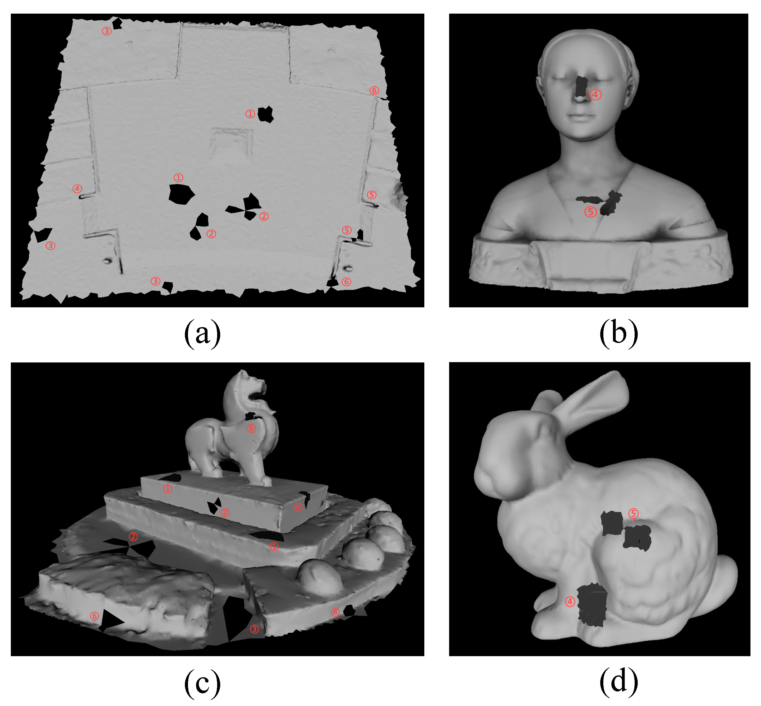
The proposed LIMOFilling is composed of four parts as shown in the Figure 3. Hole-detection occurs in the pre-processing stage, where all boundaries $S_b^i$ of all holes in the input model $M_H$ are completely collected and marked; a complex hole is decomposed into several simple holes. The holes are filled by layer-to-layer strategy during mesh-generation. The layer-to-layer strategy is a cyclic process in which the ear-clipping score is calculated in each cycle. An ear-clipping score between adjacent boundary-edges of the hole was computed to provide the position of the inserted discrete points of outermost layer of the hole which the new mesh $M_N^j$ is generated, where the planar proxies ${\phi }^s$ are updated is where the new mesh is generated. In the part of surface-fitting, the newly added mesh is adjusted locally. The generated triangles $M_N^j$ in each layer are fitted to an implicit surface, built from the existing vertices. Their normal vectors in the neighborhood of the hole-boundary act as constraints. Sharp-feature-recovery is achieved by a global adjustment for the complete newly generated mesh in the area of the hole. The planar proxies ${\phi }^s$ and the normal vectors of the triangular plane are used as a condition to constrain the adjustment.

3.1. Hole Detection

Manifold meshes are stored in a half-edge data structure because of the speed, simplicity, and high efficiency of this system. An edge is represented as two half-edges with opposite directions thus avoiding the need to distinguish the direction of polygon edges in the data structure [32]. The half-edge data structure can represent any arbitrary manifold directional polygon mesh, where the half-edges of the polygon face are consistently oriented along the counterclockwise direction. Moreover, the manifold mesh topology is maintained providing easy access for mutual searches among vertices, edges, and faces. A boundary-edge connected to previous boundary-edge is in turn connected to the next-edge along the hole border. Thus, the boundary-edges of a hole can be easily found by using the starting-vertex and ending-vertex properties of a half-edge and the boundary-edge judgment. The entire border of a hole can be collected through the boundary half-edge extension.

The boundary-edges of a hole are collected by the boundary half-edge extension directly in simple hole-detection. The method is a cyclical process, an unmarked boundary half-edge is randomly selected as the starting-vertex in the hole-detection, and this half-edge is marked. Boundary half-edges include not only the hole-boundary-edges but also the model border-edges, see Figure 4.

As seen in the diagram, the starting half-edge HE1 is a boundary half-edge from the starting-vertex FV1 to the ending-vertex TV1, the boundary half-edge extension finds a half-edge starting from the ending-vertex TV1 of the current half-edge as the extension half-edge, and TV1 is the starting-vertex FV2 of the extension half-edge. However, there are five half-edges starting from the vertex FV2, i.e., HEa, HEb, HEc, HEd, and HE2, as shown in Figure 4. However, there is only one half-edge among the five edges: HE2, is the boundary half-edge. Thus, the border of the hole is extended from HE1 to HE2, and HE2 is marked. All the boundaries of simple holes are collected by direct the boundary half-edge extension in this way.

The direct boundary half-edge extension can extend the boundary of a simple hole quickly and accurately because usually only one boundary half-edge starts from the end of a previous boundary half-edge. The presence of non-manifold vertices in a complex hole however, means that a boundary half-edge is not unique, and more than one candidate edge qualifies as a boundary-edge, unlike the situation of simple holes. A complex hole consisting of three simple holes via connected by a non-manifold vertex $V_0$, is shown in Figure 5. When the boundary half-edge extension encounters a non-manifold vertex, there is no longer only one boundary half-edge available for extension. Therefore, the problem becomes how to select an optimal extended half-edge from several candidates that satisfy the extension condition.

Hole-detection expectations clarify the direction of optimal boundary half-edge selection. A complex hole was decomposed into two or more simple holes to avoid potential problems that arise when filling complex holes directly. A complex hole consisting of three simple holes (purple, bule and yellow) via connected by a non-manifold vertex $V_0$, shown in Figure 5, where $V_0,V_1,V_2,V_3,V_4$ is the boundary vertices of purple hole, $V_0,V_5,V_6,V_7$ is the boundary vertices of blue hole and $V_0,V_8,V_9,V_{10}$ is the boundary vertices of yellow hole. Among the complex hole, HE1 and HE2 belong to the same purple simple hole, while HE3 and HE4 belong to the yellow and blue simple hole. Choosing the boundary half-edge of the same hole as the extended half-edge can open a breakthrough for solving optimal boundary half-edge selection. To select optimal half-edge, a fast and robust algorithm was designed that accurately finds the optimal extended half-edge from several candidate half-edges.

The proposed method selects the extended half-edge by judging the intersection between the auxiliary segments and the triangular surfaces around the non-manifold vertex that are closely connected with the complex hole. The auxiliary segments are constructed by connecting the starting vertex of the current half-edge to the ending vertex of all the boundary half-edges to be selected without actually adding any edge to the mesh. There are as many auxiliary segments as there are candidate half-edges. It was inferred from extensive experiments and engineering experience that, among many candidates, only a half-edge that belongs to the same simple hole as the current half-edge determines an auxiliary segment which does not intersect any triangular surface, because this auxiliary segment and its projection always lie inside this simple hole, as illustrated in Figure 5. In the figure, Sg2 intersects the triangle $\Delta V_0,V_4,V_5$ and the triangle $\Delta V_0,V_7,V_8$ in the triangular plane, and Sg3 coincides with an edge $V_4,V_5$ of the triangle $\Delta V_0,V_4,V_5$, which also considered as a case where the segment intersects the triangle. An exception is when the angle between HE1 and HE2 facing the simple hole is greater than 180°, the auxiliary segment will be outside the hole. However, the triangles connected to the exceptional non-manifold vertex are often abnormal triangles, such as spikes or degenerate triangles. To avoid anomalies, a spike and degenerate surfaces removal algorithm [33] is used during pre-processing the mesh in the proposed method.

It has to emphasize that the intersection judgment is on the triangular plane. Since the mesh is three-dimensional, the adjacent triangles do not necessarily lie strictly on one plane where there is a change in elevation. Therefore, each auxiliary segment is projected separately onto a defined plane to determine whether the segment intersects the triangle in that plane or not. To project the auxiliary segment, a local spatial coordinate system is constructed, which takes the triangular plane to be detected as the base plane. The coordinate system takes the non-manifold vertex $V_0$ as the origin, the normal n of the candidate triangular plane as the z-axis, and the plane where the triangle is located constitutes the $V_{0}xy$ plane. The coordinate axis vectors of the local coordinate system are ${\mathit{P}}_{\mathit{x}}$, ${\mathit{P}}_{\mathit{y}}$, and ${\mathit{P}}_{\mathit{z}}$, which can be expressed as follows:

$$\begin{array}{l}{\mathit{P}}_{\mathit{z}}=\mathit{n}\\ {\mathit{P}}_{\mathit{y}}=\mathit{n}\times (1,0,0)\\ {\mathit{P}}_{\mathit{x}}={\mathit{P}}_{\mathit{y}}\times {\mathit{P}}_{\mathit{z}}.\end{array}$$

(1)

A projection rotation matrix ${\mathit{R}}_p$ is formed by these three vectors, which is defined as

$${\mathit{R}}_p={\left[\begin{array}{ccc}{\mathit{P}}_{\mathit{x}}& {\mathit{P}}_{\mathit{y}}& {\mathit{P}}_{\mathit{z}}\end{array}\right]}^T.$$

(2)

The two endpoints of the auxiliary segment are projected into the local coordinate system by the following equation:

$$C_{V^{\prime }}=C_V{\mathit{R}}_p-C_{V_0},$$

(3)

where $C_{V_0}$ is the coordinates of the origin of the local coordinate system under the global coordinate system, and $C_{V^{\prime }}$ is the coordinates of the point $C_V$ in the global coordinate system under the local coordinate system.

A complex hole was decomposed into multiple simple holes and collected the boundary half-edges of all simple holes by the boundary half-edge extension as previously discussed in this section. The intersection judgment of auxiliary segments and triangular surfaces is the basis for decomposing the complex holes. The segments must be projected onto the triangular plane for intersection judgment; thus, a local spatial coordinate system was constructed and the collected hole-boundary half-edges are used as hole information for mesh generation.

3.2. Mesh Generation

Mesh generation is a part of hole-repairing and a layer-to-layer framework is proposed to fill large holes. The main idea is to refine the scope of local information when filling large holes. Specifically, it is not immediately going to the next layer after generating mesh in the current layer, but perform implicit surface fitting to the newly generated mesh of the current layer and surface fitting as detailed in Section 3.3. Mesh generation consists of two steps, discrete vertices insertion and triangulation. Many common discrete point insertion algorithms select edges randomly and are not robust for arbitrary angles [5]. In addition, ear-clipping triangulation does not guarantee the uniformity of the mesh. The algorithm was improved by introducing the ear-selection idea of ear-clipping triangulation [21] into the discrete vertices insertion and defining the priority of triangulation. The boundary set of each simple hole as collected in Section 3.1 is used in mesh generation to uniformly generate a new mesh in the hole-area.

The insertion of discrete vertices and triangulation are the main two steps of mesh-generation. The traditional methods of inserting discrete points in the hole-region, such as [34], is to randomly select a point $V_i$ from the set of hole-boundary vertices $V=\left\{V_0,V_1,V_2,\cdots \cdots ,V_n\right\}$, and calculate the location of the inserted point by the angle θ formed by the two neighboring edges associated with $V_i$ and the average length ${\overline{l}}_i$ of the two edges. Although this method inserts the discrete vertices required for hole-repairing in the hole-region, the edge-selection is random. Moreover, convex (θ > 180°) and concave (θ < 180°) angles are handled differently by those methods, so additional judgment on θ is required, which increases the complexity of the algorithm, and does not guarantee the uniform insertion of discrete points.

The vertex insertion method was improved to eliminate the randomness of edge-selection, reduce the complexity, and make the algorithm robust to arbitrary angles by introducing the ear-selection idea of ear-clipping triangulation in the proposed edge-selection method. We calculate the ear-clipping score of each ear on the edge of the hole, and select the two edges where the ear with the smallest ear-clipping score is located. The middle vertex is $V_i$, and the adjacent two vertices are $V_{i-1}$ and $V_{i+1}$. Each ear is visited only once, and after being visited the ears are not calculated in another loop. The next smallest ear is selected for calculation next time. The position coordinates of the inserted vertex of the current ear constraint are calculated by the following equation:

$$C_{v_{ip}}=\frac{C_{v_{i+1}}-C_{v_i}}{\left|C_{v_{i+1}}-C_{v_i}\right|}\cdot \left[\begin{array}{cc}\cos \kappa \delta & \sin \kappa \delta \\ -\sin \kappa \delta & \cos \kappa \delta \end{array}\right]\cdot \overline{l}+C_{v_i},$$

(4)

where $C_{v_i}$, $C_{v_{i+1}}$ and $C_{v_{ip}}$ is the coordinate of the vertex $v_i$, $v_{i+1}$ and inserted vertex, respectively, $\kappa =\frac{1}{60}\theta$, $\delta =\frac{\theta }{\kappa +1}$. The distance between the later inserted vertex and all the first inserted vertices are compared. If the distance is less than $\frac{\overline{l}}{3}$, then merge these two vertices and take the midpoint of these two vertices as the new vertex. $\overline{l}$ is the average of the boundary-edge set $E=\{e_0,e_1,e_2,\dots \dots ,e_m\}$ of the hole, calculated by the following equation:

$$\overline{l}=\frac{1}{m}{\displaystyle \sum _{j=0}^m{e}_j}.$$

(5)

A layer of discrete vertices in the hole-area is inserted when each ear has been visited. The next layer of vertices is inserted based on the new set of hole-boundary-edges $E^{\prime }$ formed after the previous layer of discrete vertices is inserted and triangulated.

It is not triangulate the insertion vertices by simply ear-clipping [21] even though it has the lowest triangulation complexity and by far the simplest triangulation method. A priority of triangulation must be defined because the position of the insertion vertex is determined by associated boundary-edge and the repair of the whole hole is layer-to-layer. The triangle formed by the added vertex and the associated boundary vertices is given priority when triangulating the discrete vertices and whether the discrete vertices can form triangles between the vertices must be considered. Only those triangles close to equilateral triangles can be accepted. The length of the ear-clipping line (the line connecting the two endpoints of the ear) was calculated, if it is less than $\frac{\overline{l}}{2}$ then it directly forms a triangle with the two edges of the ear. Otherwise, a vertex is inserted according to Equation (4), and merge the vertices whose distance is less than $\frac{\overline{l}}{3}$. 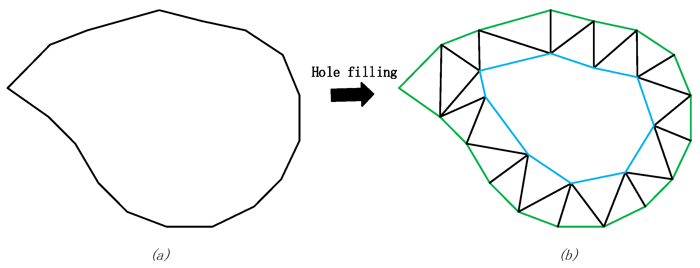The two vertices of the boundary-edge associated with the insertion point form a new triangle, in which a boundary-edge in the original mesh can only be visited once. All newly inserted vertices have to be assessed in relation to the definition. A layer of vertices inserted and triangulated is displayed in Figure 6.

In Figure 6, the green border is the boundary of the origin hole. The hole-boundary of the next layer is formed by a layer of inserted and triangulated vertices, as indicated by the blue line. The proposed method does not distinguish between concave and convex angles when selecting edges. As illustrated, the proposed mesh generation method guarantees the uniformity of the inserted vertices, and generates regular triangular surfaces.

Planar proxies for the original mesh are extracted before filling the holes; the aim is to sense the structure of the model. Two or more adjacent triangular surfaces can be approximated to some extent by a simple plane φ [35,36,37], called a planar proxy. The planar proxies of the model are obtained by the region-growing method. The local tangent plane and flatness score of each triangular surface t is estimated by selecting a linear-least-squares fitting to the planes on a point set that is chosen as a subset of the mesh vertices in the local neighborhood. The latter is set as the set of triangular faces t in a noiseless dataset and as a larger combined neighborhood in a noisy dataset. Immediately afterwards, the current region is iteratively grown, operating on one region at a time, always selecting the triangle with the lowest flatness score not being used for the growth of a particular region, as the cell for region growth. A planar proxy was obtained by the region growing method. Each region grows on the surface of adjacent triangles, one triangle at a time. The angle between the normal vector of this triangle (the line perpendicular to the plane of the triangle) was computed, the normal vector of the seed plane (the line perpendicular to the seed plane) and the Euclidean distance between them. If both metrics are simultaneously smaller than a given threshold, then this triangle is accepted as a unit of region growth. Notably, the seed plane is not recalculated during the growth of a region. After an iteration is completed, if the total area of the resulting set of faces is less than the threshold area, the region is rejected; otherwise, each triangle can be detected as a planar proxy. After growing the area for the whole model, adjacent faces that are approximately co-planar are merged into a plane. The planar proxies are represented by the set of triangles ${\phi }_1=\left\{t_1^1,t_2^1,t_3^1,\dots \dots ,t_m^1\right\}$, ${\phi }_2=\left\{t_1^2,t_2^2,t_3^2,\dots \dots ,t_n^2\right\}$,……,${\phi }_k=\left\{t_1^k,t_2^k,t_3^k,\dots \dots ,t_q^k\right\}$ that belong to the same planar proxy, implying that the model extracts a total of k planar proxies, with m, n, ......, q triangles belong to different planar proxies. One triangle belongs to only one planar proxy, and there are triangles that do not belong to any planar proxy.

The meshes in hole-region were generated by layer-to-layer for filling large holes and introduce the ear-selection idea in ear-clipping triangulation in the vertices insertion process to improve the algorithm, as well as to define the priority of triangulation to ensure the uniformity of the inserted vertices. Planar proxies are extracted before mesh generation to obtain a sense of the structure. Generated mesh surfaces are fitted to ensure a smooth transition between the old and new meshes and to repair the highly curved holes.

3.3. Surface Fitting

To ensure a smooth-transition between the old and new meshes and to repair the highly curved holes, surface-fitting is performed after mesh generated. An implicit surface is constructed for surface-fitting and the position of the newly generated mesh is adjusted based on the implicit surface. An implicit surface was constructed based on the radial basis function. It has high order continuity for multiple scattered data point interpolation, and contains only one independent variable representing distance so that complex surfaces with arbitrary topologies can be obtained. There are many expressions for radial basis functions in practical surface reconstruction; Carr et al. give a list of the expressions and a detailed analysis of their applicability [38]. The proposed implicit surface method is a fit to a function containing three variables, so the multiple reconciliation function $h(r)={\Vert r\Vert }^3$ is used. The surface-fitting is another part of hole-repairing.

The surface representation is defined as finding a surface $M^{\prime }$ to approximately represent the surface M for multiple points of the surface M that differ in space [39]. An implicit surface can be defined as: finding a function $f(x,y,z)$ such that any point of the surface $M^{\prime }$ satisfies $f(x,y,z)=0$. The function $f(x,y,z)$ is said to implicitly define the surface $M^{\prime }$. Suppose there is a discrete vertex set $V_{Disc}=\{v_0,v_1,v_2,\dots \dots ,v_n\}$ in the space, and each point of the set has corresponding constraint set $Cons=\left\{c_0,c_1,c_2,\dots \dots ,c_n\right\}$. For the discrete vertices in the space, if a function $f(r)$ can be constructed so that each discrete vertex satisfies $f(v_i)=c_i$, then these n discrete vertices can also define an implicit surface $f(v_i)=0$. The surface over the set of discrete points with constraint values c = 0.

Work in [38] and [39] of constructing implicit surfaces based on radial basis functions is useful for repair of simple structures and small size holes. However, when a hole is large, relying only on the vertices of the hole edges as constraint vertices cannot accurately describe the structure of the hole-area. Nevertheless, the implicit surface constraint weakens as the distance from the edge of the hole increases, as the center of the hole might be too far from the constraint vertices. Thus, surface-fitting was performed in a layer-to-layer framework introduced in Section 3.2. The implicit surface of the current layer is constructed by a set of collaborative constraint vertices, which composed by the hole-boundary vertices and the discrete points inserted in the current layer and the surface can be expressed as:

$$f(r)={\displaystyle \sum _{j=1}^n{w}_{j}h(\Vert r-v_j\Vert )}+\varphi (r),$$

(6)

where $v_j$ is a constraint vertex, and $w_j$ is the weight of each sampling vertex. $\varphi (r)$ is the residual function whose role is to maintain the affine invariance of the input points, which is defined as

$$\varphi (r)=p_0+p_{1}x+p_{2}y+p_{3}z,$$

(7)

where x, y, and z are the three-dimensional coordinates of the spatial vertex and $p_0,p_1,p_2,p_3$ is the function coefficient. $h(r-v_j)$ is the radial basis function chosen to construct the implicit surface, which takes the form of $h(r)={\Vert r\Vert }^3$ when interpolating the sampling vertices in three-dimensional space.

Furthermore, the selection principle of constraint vertices and the method for solving implicit surfaces assume that for a constraint vertex $v_i$, if that satisfies $f(v_i)=0$, the point is on the surface, and undoubtedly considered the surface constraint vertex. Otherwise, the vertex is not on the surface (where, if $f(v_i)<0$, the vertex is inside the surface; if $f(v_i)>0$, the vertex is outside the surface), which is said to be a non-surface constraint vertex. Since the implicit surfaces are constructed by layer to layer, the insertion point of current layer is selected as the constraint vertex in each loop. Moreover, any vertex that deviates from each surface constraint vertex by a 0.5 directional length, is selected as the non-surface constraint vertex. If the constraint is given as $c_i=f(v_i)$, to solve for the four coefficients $p_0,p_1,p_2,p_3$ of residual function and the weight $w_j$, two conditions need to be satisfied:

(1) The interpolation constraint, expressed as

$$f(v_i)={\displaystyle \sum _{j=1}^n{w}_{j}h(\Vert v_i-v_j\Vert )}+\varphi (v_i)=c_i.$$

(8)

(2) The energy orthogonality, denoted as

$${\displaystyle \sum _{j=1}^n{w}_j}={\displaystyle \sum _{j=1}^n{w}_j{v}_j^x}={\displaystyle \sum _{j=1}^n{w}_j{v}_j^y}={\displaystyle \sum _{j=1}^n{w}_j{v}_j^z}=0,$$

(9)

where, j = 1, 2, 3, ......, n. Let $h_{ij}=h(v_i-v_j)$, the system of linear equations can be obtained from Equations (8) and (9), that expressed as

$$\left[\begin{array}{cccccccc}{h}_{11}& h_{12}& \dots & h_{1n}& 1& v_1^x& v_1^y& v_1^z\\ h_{21}& h_{22}& \dots & h_{2n}& 1& v_2^x& v_2^y& v_2^z\\ \dots & \dots & \dots & \dots & \dots & \dots & \dots & \dots \\ h_{n1}& h_{n2}& \dots & h_{nn}& 1& v_n^x& v_n^y& v_n^z\\ 1& 1& \dots & 1& 0& 0& 0& 0\\ v_1^x& v_2^x& \dots & v_n^x& 0& 0& 0& 0\\ v_1^y& v_2^y& \dots & v_n^y& 0& 0& 0& 0\\ v_1^z& v_2^z& \dots & v_n^z& 0& 0& 0& 0\end{array}\right]\left[\begin{array}{c}{w}_1\\ w_2\\ \dots \\ w_n\\ p_0\\ p_1\\ p_2\\ p_3\end{array}\right]=\left[\begin{array}{c}{c}_1\\ c_2\\ \dots \\ c_n\\ 0\\ 0\\ 0\\ 0\end{array}\right].$$

(10)

In Equation (10), the matrix on the left side of the equal sign is a positive definite matrix, yielding a unique solution $(w_1,w_2,\dots \dots ,w_n,p_0,p_1,p_2,p_3)$. Substituting the solution of the equation into the definition formula Equation (6), the implicit surface equation can be solved as

$$f(x,y,z)={\displaystyle \sum _{j=1}^n{w}_j{(\sqrt{{(x-v_j^x)}^2+{(y-v_j^y)}^2+{(z-v_j^z)}^2})}^3}+p_0+p_{1}x+p_{2}y+p_{3}z.$$

(11)

Further, the newly generated mesh is fitted to the implicit surface by adjusting the position of the triangles. A method was introduced for adjusting triangles. The triangle is adjusted by three vertices gradually approaching the implicit surface along the gradient direction, which is expressed as

$$\nabla f=(\frac{\partial f}{\partial x},\frac{\partial f}{\partial y},\frac{\partial f}{\partial z}).$$

(12)

Additionally, calculate the first-order partial derivative of Equation (11), the following equation is obtained:

$$\begin{array}{l}\frac{\partial f}{\partial x}=3{\displaystyle \sum _{j=1}^n{w}_j(x-v_j^x)\cdot {(\sqrt{{(x-v_j^x)}^2+{(y-v_j^y)}^2+{(z-v_j^z)}^2})}^3}+p_1\\ \frac{\partial f}{\partial y}=3{\displaystyle \sum _{j=1}^n{w}_j(y-v_j^y)\cdot {(\sqrt{{(x-v_j^x)}^2+{(y-v_j^y)}^2+{(z-v_j^z)}^2})}^3}+p_2,\\ \frac{\partial f}{\partial z}=3{\displaystyle \sum _{j=1}^n{w}_j(z-v_j^z)\cdot {(\sqrt{{(x-v_j^x)}^2+{(y-v_j^y)}^2+{(z-v_j^z)}^2})}^3}+p_3\end{array}$$

(13)

A triangle vertex that finally reaches a point on that implicit surface is called the mapping point of the vertex. The coordinates of the mapping point on the implicit surface can be calculated by the following equation:

$$C_{v_m}=C_{v_o}-\frac{f(v_o)}{{\Vert \nabla f(v_o)\Vert }^2}\nabla f(v_o),$$

(14)

where $C_{v_o}$ is the coordinate of vertex $v_o$ before position adjustment, and $C_{v_m}$ is the 3D coordinate of mapping point $v_m$, which is also the coordinate of $v_o$ after adjustment. The adjustment distance was also calculated; if the distance is less than the minimum threshold, it was considered that $v_o$ originally belongs to a vertex on the implicit surface, and does not need to adjust the position. Otherwise, the vertex position needs to change. Newton’s method is used to perform the vertices position adjustment; this is an iterative merit-seeking method that allows a certain function to approach the target vertex as fast as possible from the negative gradient direction of the vector [40].

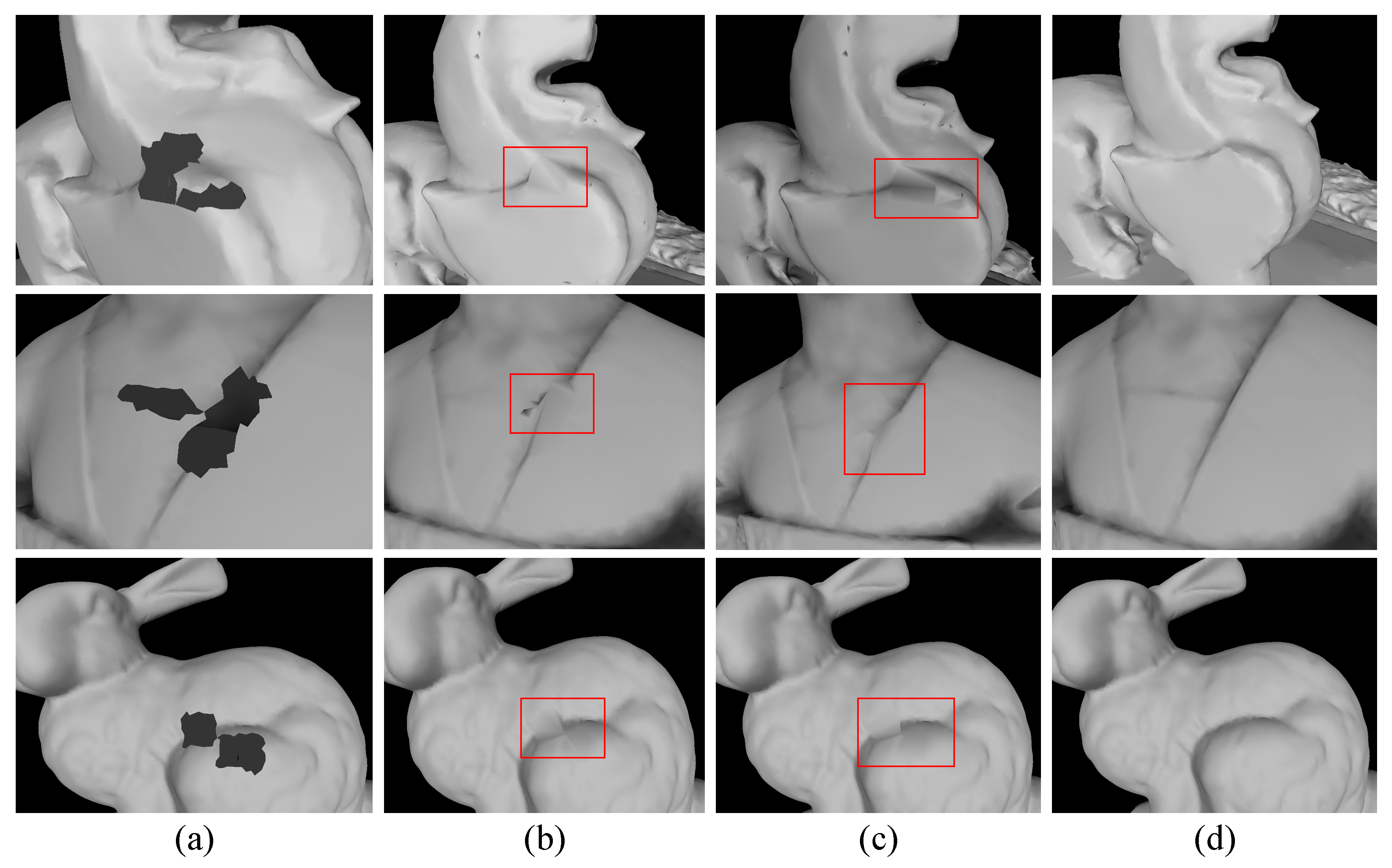
The newly generated mesh satisfies the requirement of smooth transition between the old and new meshes after fitting all the inserted vertices to the implicit surface. The set of planar proxies ${\phi }^s$ is updated by assigning triangles to each planar proxy or not to any planar proxy, which according to the deviation between the normal vectors of the adjusted triangle and the planar proxy. Figure 7 shows the hole-repairing result of the hole in Figure 6.

The proposed method in Figure 7c has advantages over the two typical hole-filling methods shown in Figure 7a,b. The non-negligible drawback of the method without inserting any vertices (Figure 7a) is that the resulting triangles shape is usually narrow, with a considerable impact on the recovery of the feature structure. The discrete vertices inserted by layer-to-layer, as in Figure 7c, are more evenly distributed within the hole-area than those inserted by the one-time hole-filling method, which are more concentrated in the center of the hole. Moreover, the one-time hole-filling method produces degenerated triangles whose shapes are approximately a line, as indicated by the red box in Figure 7b. The proposed approach however, eliminates the possibility of creating degenerate triangles at the algorithmic level, thus yielding only regular triangles, as shown in Figure 7c.

The newly generated meshes were fitted by constructing an implicit surface based on radial basis function. The newly generated mesh is adjusted based on the implicit surface. Surface fitting smooths the transition between old and new mesh; subsequently, the highly curved holes can be repaired in the feature recovery process. The sharp features of a hole however, cannot be recovered by implicit surface fitting, thus structural information from the planar proxies is applied in feature recovery.

3.4. Feature Recovery

The planar proxies were introduced to recover the sharp features of the mesh after implicit surface fitting by adjusting the positions of the triangles. Figure 8 shows the planar proxies of the sharp features and their restored models. The triangular faces in the same plane proxy have similar normal directions, and this rule is followed to continuously update the plane proxies during mesh generation. The overlay of the planar proxies before and after the hole-filling as shown in Figure 8c,f, precisely presenting the recovered sharp features. Position adjustment in the feature recovery process is different from that in surface fitting as normal triangle vector information and planar proxies are considered in the proposed feature recovery method. Specifically, on the basis of grid-based mean filtering, the joint constraints were constructed using the normal triangle vectors around the triangle to be adjusted and the normal planar proxy containing the triangle [41]. The proposed feature recovery method is an iterative optimization process.

For a triangular surface $t$ with normal vector $n_t$, the set of triangular surfaces in the one-loop neighborhood of $t$ is $T=\{t_1,t_2,t_3,\dots \dots ,t_m\}$, and the corresponding set of normal vectors is $N_t=\{n_1,n_2,n_3,\dots \dots ,n_m\}$. Weighting each triangle within a one-ring neighborhood of the triangle $t$ by the following equation:

$$w_i={\varphi }_{ti}{}^2\cdot {\varphi }_{t\phi },$$

(15)

where ${\varphi }_{ti}$ is the cosine of the angle between the normal of $t$ and neighboring triangle $t_i$, which when expressed as $cos\angle \left(t,t_i\right)\in \left(0,1\right)$, $i=1,2,3,\dots \dots ,m$. ${\varphi }_{t\phi }$ is the cosine of the angle between $t$ and the planar proxy ${\phi }_j$ to which $t$ belongs, and if $t$ does not belong to any planar proxy, the value ${\varphi }_{t\phi }=1$. The smaller the deviation of the normal of the triangle from the normal of $t$, the larger the weight, and vice versa when the deviation of the normal of the triangle is bigger from the normal of $t$, the smaller the weight. The position of each vertex $v_j^{bef}$ in the triangle surface $t$ is adjusted by the following equation:

$$C_{v_j^{adj}}=C_{v_j^{bef}}+\frac{1}{{\displaystyle \sum _{i=1}^m{w}_i}}{\displaystyle \sum _{i=1}^m{w}_i(C_{v_j^{bef}}-C_{c_t})}\cdot n_i,$$

(16)

where $C_{v_j^{adj}}$ is the adjusted coordinate of vertex $v_j^{bef}$ in $t$, j is the current number of iterations, and $C_{c_t}$ is the center of gravity coordinate of $t$ before position adjustment. After updating the coordinates of the three vertices of the triangular surface, the center of gravity coordinate is updated accordingly. In addition, the normal of the triangular surface after the position adjustment is recalculated by the following equation:

$$n_t^{new}=\frac{1}{{\displaystyle \sum _{i=1}^m{w}_i}}{\displaystyle \sum _{i=1}^m{w}_i}{n}_i.$$

(17)

If $\Vert C_{v_j^{adj}}-C_{v_{j-1}^{adj}}\Vert <0.001$, stop the iteration, otherwise the position optimization is continued, where $C_{v_{j-1}^{adj}}$ is the vertex coordinate after the last loop adjustment.

The features were recovered by triangles adjustment constrained by triangles normal vector information and planar proxies. This information is works by weighting different triangles vertices to obtain the structural features of the holes. Notably, if a triangle does not belong to any planar proxy, then it is only considered in relation to the triangle and with the surrounding triangles. A series of experiments were designed to investigate the hole-filling ability of the proposed method.

4. Experiments

In experiments, the proposed LIMOFilling was applied for filling various holes on 3D models. In this section, the hole-filling results are presented and compared with the results from other hole-filling methods from the MeshFix proposed by Attene [42] and the Visualization and Computer Graphics (VCG) library [43]. The VCG library is tailored to manage triangular meshes and offers many states of the art functionalities for processing meshes, such as hole-detection and mesh-repairing capabilities. A number of applications have been developed using the VCG library, such as MeshLab, but the proposed hole-filling method provides a general method for a given manifold mesh with holes. The comparative experiments tested the ability of the different methods to detect and repair arbitrary forms of holes that may be present in a model for any scene, as well as the ability to recover sharp features of a hole. It is also interesting to explore the efficiency of each method in handling the holes and the quality of the generated triangular surfaces.

To investigate the hole-filling ability of the proposed method, the following experiments were conducted. Hole-detection was performed on different types of scene models. Some of the holes in models were caused by occlusion during data collection and some other factors, while others were created manually to better demonstrate the effect of the proposed method. To intuitively reflect the difference in detection capability for different types of holes, the repaired results were shown, since the holes are not repaired if they are not detected. We compared the repair results of the different methods on complex holes to test whether the hole-filling method causes the overlap between the triangles. The sharp features recovery effect was qualitatively evaluated by the filled results. The proposed hole-detection method decomposes a complex hole into many, while the VCG method and the MeshFix deploy the method similar to the boundary half-edge extension to collect the boundaries of a hole for filling. A quantitative hole-detection experiment was designed using a model with a countable number of holes to evaluate the effectiveness of the different hole-detection approaches. The number of holes detected by the proposed hole-detection method was compared with the number of holes detected by the VCG method and the MeshFix to verify the robustness of the proposed method to different types of the holes. Further, the time consumption of the different hole-detection algorithms was compared, and we quantitatively evaluated the detection efficiency. A quantitative experiment was designed to evaluate the hole-filling accuracy. Furthermore, the quality of the newly generated triangles of the proposed hole-repairing method was evaluated by computing the specific ratio of the triangle. To increase the credibility of the experiments, any acceleration to the proposed method was not added, the input experimental data were consistent, the maximum number of allowed hole boundary edges N = 50, and all other parameters are kept constant using system default values unless stated otherwise.

4.1. Qualitative Evaluation

The holes on model boundary could not identified by the hole detection method in the VCG library and the MeshFix, but the proposed method accurately extracted the borders of such holes. The VCG hole detection method directly treats a complex hole as a simple hole using the relative position relationship between vertices, edges, and faces. The VCG method connects the borders of a boundary hole to the model boundary. The MeshFix uses a hole detection algorithm similar to the VCG. There is usually a constraint on the boundary length or number of a hole however, to avoid identifying the model boundary as a large hole. As a result, holes connected to the model boundary tend to be filtered out. Therefore, the VCG and the MeshFix hole detection method cannot identify the boundary holes, as shown in Figure 9a,b,d,e.

The filled models shown in Figure 9 visualize the detection results. Holes are not repaired if they are not detected. The gaps reflect the deficiencies of the VCG method and the MeshFix method in detecting boundary holes, as indicated by red boxes in the Figure 9. In the proposed hole-detection method, the boundary holes were detected, Figure 9c,f. A boundary hole from the model boundary was separated by decomposing the hole. Thus, a separated boundary hole is a simple hole in a decomposed hole, so its borders not stick to the model boundary when collecting borders using the boundary half-edge extension, therefore the hole is not filtered out. Filling separate simple holes avoids the trouble caused by directly filling the complex holes, there are no gaps in the repaired models by the proposed method, as shown is Figure 9c,f. The hole-filling results were further compared using the different methods in Figure 10.

The triangular surfaces overlap each other when filing highly curved holes using VCG method and MeshFix. This is shown by the red box in Figure 10b,c. When a complex hole is viewed as multiple simple hole-regions, the triangular surfaces overlap because vertices or edges across the region become associated when new triangles are generated. The proposed method decomposes the complex holes and ensures the independence of each simple hole, thus eliminating the possibility of cross-regional correlation. Therefore, overlapping triangles are avoided using the proposed hole-filling method, as indicated in Figure 10d.

In the proposed method, a complex hole is decomposed into several simple holes, of which holes are repaired by a layer-to-layer repairing strategy, and an implicit surface is constructed at each layer to fit the newly generated mesh, all reflecting the idea of divide-and-conquer. The layer-to-layer repair strategy extends the surface structure properties preserved around the holes to a certain extent to the hole-repairing. The strategy not only makes recovers sharp features possible, but also directly ensures a smooth transition between the old and new mesh. The repair results of the layer-to-layer strategy were demonstrated, as shown in Figure 11.

The repair of the holes shown in Figure 11a,e were compared the VCG hole-repairing method and MeshFix with the proposed LIMOFilling. Although the VCG method repair the hole, the unsmooth transition gives Laurana a flat nose and blurred leg contours of the Bunny, as shown in the red box in Figure 11b,f. The reason is that the structural properties remained of the mesh around the hole are not considered in mesh generation, but simply a one-time vertices insertion and triangulation are performed. MeshFix fills the holes and repairs some of the features to some extent, as shown in Figure 11c,g, but the features in the center of the holes are still difficult to be repaired because the boundary information gradually weakens the constraints on the inside of the holes. In the proposed method, the implicit surface fitting allows the old and new meshes to have consistent surface features, and the layer-to-layer strategy makes the surface constraints tighter, the hole-repairing result gained by the proposed method is shown in Figure 11d,h. However, there are errors in the implicit surface construction. The errors are accumulated when there are too many layers. Statistically, the maximum number of layers in the experiments is no more than four layers.

The proposed method recovers sharp features in a hole-region. The sharp features, such as the edge and sharp corner of the guardrail, were restored by the feature recovery method. The different methods for recovering sharp features were compared, the results are shown in Figure 12.

The proposed method compensates for the shortcomings of the VCG method and the MeshFix method by extending the feature attributes retained around the hole as local constraints to adjust the position of the newly generated mesh. In Figure 12, the red boxes highlight the results of the VCG method and the MeshFix method, and green boxes in the figure highlight the results from the proposed method for sharp feature recovery. Comparing the recovery results in Figure 12b,d, the VCG method does not restore the sharp corner of the guardrail, which reduces the authenticity of the model. Similarly, the filling result of guardrail edge also has a structural defect, which is manifested as an edge collapse, as shown in Figure 12f,h. MeshFix still has not been able to repair the sharp corners of the guardrail, but to a certain extent repairs the feature of the guardrail edge. Compared with the sharp feature recovery results of LIMOFilling, the results of MeshFix are still not satisfactory. The experiments show that the proposed method is effective.

4.2. Quantitative Evaluation

The efficiency of the different methods was investigated by comparing the time consumption. The time consumption and the number of holes detected by the different hole-detection algorithms for different data are shown in

Table 1. Number of holes detected and system efficiency comparisons between different methods.

Data	Method	Number of Holes Detected	Hole Detection Time Assumption (ms)	System Time Assumption (ms)
WCGC-S	VCG	7	113.67	337.86
	MeshFix	7	106.78	321.12
	LIMOFilling	18	122.56	1124.60
Pixiu	VCG	6	39.97	201.45
	MeshFix	6	37.88	189.76
	LIMOFilling	13	45.21	324.57
Laurana	VCG	2	176.44	357.83
	MeshFix	2	165.03	338.11
	LIMOFilling	3	185.43	625.02
Bunny	VCG	2	196.56	512.13
	MeshFix	2	178.20	490.03
	LIMOFilling	3	201.81	693.49

. A comparison of hole-filling efficiency by counting the elapsed time is only meaningful under the condition that the number of holes to be filled is the same, and why the number of holes detected was counted. The number of holes detected by the different hole-detection algorithms tested the integrity of the different methods for detecting holes.

Hole-filling is the fast process in 3D reconstruction, usually completed in a few seconds. By comparing the time consumption of different hole-detection algorithms, it is concluded that the efficiency of LIMOFilling is comparable to the VCG method and the MeshFix method. The overall efficiency of the proposed method is slightly lower than that of the two hole detect algorithms because of the time cost for constructing the local coordinate and intersection detection. However, the time difference is very small—only within 10 ms. Furthermore, a comparison of the hole-detection time consumption of Pixiu and Laurana (Laurana’s mesh is denser than that of Pixiu) showed that the efficiency of the different algorithm depends on the number of hole boundaries rather than the length of the hole boundaries. A further comparison of the time consumption of the hole-filling of the two data sets shows that the density of the mesh also affects the repair and feature recovery of the holes. These inferences can serve as a reference for subsequent method improvements, for example, when simplifying a mesh before hole-filling.

In terms of the overall hole-filling and sharp feature recovery system, the time consumption of the proposed method is almost always more than twice that of the VCG method and the MeshFix method. One reason is that the two hole-detection methods miss boundary holes, as shown in the qualitative experiments. In addition, the proposed hole-filling method introduces implicit surface fitting and feature recovery modules, which are not available in the VCG and the MeshFix. However, the time cost associated with the two modules is not obvious on the flat region, as evidenced by the close time consumption of the different methods on the Pixiu test model because there are no sharp features to repair and no implicit surface fitting is necessary. The proposed hole-repairing method is layer-to-layer, which brings a non-negligible time cost. Furthermore, a factor affecting the efficiency of the proposed method is the hole decomposition strategy. Filling more holes in the same way undoubtedly increases the consumption of time. Although the efficiency of the proposed method needs to be improved, the time consumption is still controlled within an acceptable range.

Another quantitative experiment compared the distances between the mesh of the model and the point cloud of the reference model with the help of the tool named CloudCompare. This tool calculated the Mean Distance (M.D.) and Standard Deviation (S.D.) of the distances between the model and the mesh for each method expressing the degree of fit between the two meshes. The differences between the two models, are visualized as colors with a clear color contrast, as shown in Figure 13. The mean distance and standard deviation from the point cloud to the mesh were labeled below each comparative result.

Figure 13 demonstrates that the proposed method fills the model holes more accurately than VCG and MeshFix. Since the M.D. and S.D. between the model filled by LIMOFilling and the true value are at least one orders of magnitude smaller than those between the model filled by VCG or MeshFix and the true value. This means that the holes filled using the proposed method are closer to the true value than the holes filled by VCG and MeshFix. Although the two methods also fill the holes in the model except for the boundary holes, no sharp features are recovered, as reflected by the lower fit of the filled model to the original model, that is, the larger relative distance. Conversely, the distance between the filled model by the proposed method and the original model is very small, as shown in the Figure 13c,d,i. Notably, the proposed method differs from some reconstruction-based methods [9,10] as it only acts strictly on the model holes and does not have any effect on the regions outside the holes, even if the filling of the holes is not as effective as desired. This kind of method guarantees the independence of hole filling. Another point of interest is that the hole filling results for flat surfaces is generally more effective than holes located on undulating surfaces. This is because there are no sharp features to recover on flat surfaces. This also confirms the ability of the proposed method to restore sharp features.

To ensure the quality of the newly generated mesh by LIMOFilling, the method proposed by Leong et al. [44] was used to evaluate the triangular surfaces generated by the proposed method. If the ratio of the inscribed circle diameter to the circumscribed circle diameter of the triangle surface is close to r = 1, means the triangle surface is similar to an equilateral triangle. Generally, triangles with a ratio r > 0.5 are considered to be of high quality. The relevant quality evaluation metrics of the newly meshes generated by the proposed hole-filling method were counted as shown in

Table 2. Newly added triangles quality assessment.

Data	Total Number of Triangles	Number of New Triangles	Number of the New Triangles with r < 0.5	Average Ratio of the New Triangles
WCGC-S	15,449	467	4	0.9345
Pixiu	124,563	3752	13	0.9549
Laurana	50,078	1666	7	0.9413
Bunny	34,648	2169	9	0.9432

.

A series of quality evaluation indicators include the total number of triangles contained in the filled model, the number of new triangles, and the average quality of the new triangles. Furthermore, the number of the new triangles with r < 0.5 were also counted. Table 2 shows the average quality is r > 0.9, and close to r = 1, and r < 0.5 less than 1% of the total number of new triangles. These statistical results show that the proposed method not only completes the hole-filling task effectively, but also guarantees the high quality of the newly generated triangles.

5. Conclusions

Hole-filling is an active research topic in the field of 3D reconstruction. The main contribution of this paper was to build a new hole-filling and sharp feature recovery method, for manifold mesh models. In this paper, complex holes are decomposed into multiple simple holes to fill by constructing local overlap judgment. The proposed hole-detection method maintains the independence of each simple hole and fundamentally avoids the overlap between triangular surfaces. The newly generated meshes are fitted using an implicit surface constructed based on radial basis functions that extends the structural feature properties preserved by the mesh around the hole to the hole-repairing. This provides a possibility for feature-recovery, while ensuring a smooth-transition between the old and new meshes. Hole-repairing is performed in a layer-to-layer framework, which exploits local information to effectively constrain the central region of the hole, but with attendant time costs. A feature-recovery algorithm was designed to restore the original features of the holes on the basis of the repaired holes. Experimental results showed that the expected results were achieved.

There are several ways in which the system could be extended; a clear possibility is to improve method efficiency. The layer-to-layer strategy does improve the model restoration to a great extent; however, efficiency becomes a big problem because of the need to iteratively calculate the locations of insertion vertices and triangulation although constructing the implicit surface for each layer is also an iterative process, less time consuming than the vertices insertion and triangulation. Addressing vertices insertion issues further, the edges of the previous layer can be used to make predictions about the ear-clipping score of the next layer, and thus estimate the locations of the insertion vertices in the next layer. The density of the meshes is also one of the factors affecting hole-filling, so proper mesh simplification before filling is also one of the ways to improve the efficiency of the proposed method.

References

1. Altantsetseg, E.; Khorloo, O.; Matsuyama, K.; Konno, K. Complex hole-filling algorithm for 3D models. In Proceedings of the Computer Graphics International Conference, Yokohama, Japan, 27–30 June 2017; pp. 1–6. [Google Scholar] [CrossRef]
2. Lhuillier, M.; Yu, S. Manifold surface reconstruction of an environment from sparse Structure-from-Motion data. Comput. Vis. Image Underst. 2013, 117, 1628–1644. [Google Scholar] [CrossRef] [Green Version]
3. Kazhdan, M.; Hoppe, H. Screened Poisson Surface Reconstruction. ACM Trans. Graph. 2013, 32, 61–67. [Google Scholar] [CrossRef] [Green Version]
4. Kolluri, R.; Shewchuk, J.R.; O’Brien, J.F. Spectral Surface Reconstruction from Noisy Point Clouds. In Proceedings of the 2004 Eurographics/ACM SIGGRAPH Symposium on Geometry Processing, Nice, France, 8–10 July 2004; pp. 11–21. [Google Scholar] [CrossRef] [Green Version]
5. Guo, X.; Xiao, J.; Wang, Y. A survey on algorithms of hole filling in 3D surface reconstruction. Vis. Comput. 2018, 34, 93–103. [Google Scholar] [CrossRef]
6. Weber, C.; Hahmann, S.; Hagen, H. Sharp feature detection in point clouds. In Proceedings of the 2010 Shape Modeling International Conference, Aix-en-Provence, France, 21–23 June 2010; pp. 175–186. [Google Scholar] [CrossRef] [Green Version]
7. Attene, M.; Campen, M.; Kobbelt, L. Polygon Mesh Repairing: An Application Perspective. ACM Comput. Surv. 2013, 45, 1–33. [Google Scholar] [CrossRef]
8. Davis, J.; Marschner, S.R.; Garr, M.; Levoy, M. Filling holes in complex surfaces using volumetric diffusion. In Proceedings of the First International Symposium on 3D Data Processing Visualization and Transmission, Padua, Italy, 19–21 June 2002; pp. 428–441. [Google Scholar]
9. Ju, T. Robust Repair of Polygonal Models. ACM Trans. Graph. 2004, 23, 888–895. [Google Scholar] [CrossRef] [Green Version]
10. Nooruddin, F.S.; Turk, G. Simplification and repair of polygonal models using volumetric techniques. IEEE Trans. Vis. Comput. Graph. 2003, 9, 191–205. [Google Scholar] [CrossRef] [Green Version]
11. Harary, G.; Tal, A.; Grinspun, E. Context-Based Coherent Surface Completion. ACM Trans. Graph. 2014, 33, 1–12. [Google Scholar] [CrossRef]
12. Liepa, P. Filling Holes in Meshes. In Proceedings of the 2003 Eurographics/ACM SIGGRAPH Symposium on Geometry Processing, Aachen, Germany, 23–25 June 2003; pp. 200–205. [Google Scholar] [CrossRef]
13. Pernot, J.-P.; Moraru, G.; Véron, P. Filling holes in meshes using a mechanical model to simulate the curvature variation minimization. Comput. Graph. 2006, 30, 892–902. [Google Scholar] [CrossRef] [Green Version]
14. Bischoff, S.; Kobbelt, L. Structure Preserving CAD Model Repair. Comput. Graph. Forum 2005, 24, 527–536. [Google Scholar] [CrossRef]
15. Floater, M.S.; Reimers, M. Meshless parameterization and surface reconstruction. Comput. Aided Geom. Des. 2001, 18, 77–92. [Google Scholar] [CrossRef]
16. Franc, M.; Skala, V. Fast Algorithm for Triangular Mesh Simplification Based on Vertex Decimation. In Proceedings of the Computational Science—ICCS 2002; Sloot, P.M.A., Hoekstra, A.G., Tan, C.J.K., Dongarra, J.J., Eds.; Springer: Berlin/Heidelberg, Germany, 2002; pp. 42–51. [Google Scholar] [CrossRef] [Green Version]
17. Huang, X.; Xiaoguang, C.; Jianya, G. Side Ratio Constrain Based Precise Boundary Tracing Algorithm for Discrete Point Clouds. Int. Arch. Photogramm. Remote Sens. Spat. Inf. Sci. 2008, 37, 349–354. [Google Scholar]
18. Brunton, A.; Wuhrer, S.; Shu, C.; Bose, P.; Demaine, E.D. Filling holes in triangular meshes by curve unfolding. In Proceedings of the 2009 IEEE International Conference on Shape Modeling and Applications, Beijing, China, 26–28 June 2009; pp. 66–72. [Google Scholar] [CrossRef]
19. Hu, P.; Wang, C.; Li, B.; Liu, M. Filling Holes in Triangular Meshes in Engineering. JSW 2012, 7, 141–148. [Google Scholar] [CrossRef]
20. Zhao, W.; Gao, S.; Lin, H. A robust hole-filling algorithm for triangular mesh. Vis. Comput. 2007, 23, 987–997. [Google Scholar] [CrossRef]
21. Eder, G.; Held, M.; Palfrader, P. Parallelized ear clipping for the triangulation and constrained Delaunay triangulation of polygons. Comput. Geom. 2018, 73, 15–23. [Google Scholar] [CrossRef]
22. Verdera, J.; Caselles, V.; Bertalmio, M.; Sapiro, G. Inpainting surface holes. In Proceedings of the 2003 International Conference on Image Processing (Cat. No.03CH37429), Barcelona, Spain, 14–17 September 2003; Volume 2, pp. 903–906. [Google Scholar]
23. Barequet, G.; Sharir, M. Filling gaps in the boundary of a polyhedron. Comput. Aided Geom. Des. 1995, 12, 207–229. [Google Scholar] [CrossRef]
24. Branch, J.; Prieto, F.; Boulanger, P. Automatic Hole-Filling of Triangular Meshes Using Local Radial Basis Function. In Proceedings of the Third International Symposium on 3D Data Processing, Visualization, and Transmission (3DPVT’06), Chapel Hill, NC, USA, 14–16 June 2006; pp. 727–734. [Google Scholar] [CrossRef]
25. Kumar, A.; Shih, A.; Ito, Y.; Ross, D.; Soni, B. A Hole-filling Algorithm Using Non-uniform Rational B-splines. In Proceedings of the 16th International Meshing Roundtable; Brewer, M.L., Marcum, D., Eds.; Springer: Berlin/Heidelberg, Germany, 2008; pp. 169–182. [Google Scholar] [CrossRef]
26. Wang, J.; Oliveira, M.M. Filling holes on locally smooth surfaces reconstructed from point clouds. Image Vis. Comput. 2007, 25, 103–113. [Google Scholar] [CrossRef]
27. Liu, S.; Wang, C.C.L. Quasi-interpolation for surface reconstruction from scattered data with radial basis function. Comput. Aided Geom. Des. 2012, 29, 435–447. [Google Scholar] [CrossRef]
28. Sharf, A.; Alexa, M.; Cohen-Or, D. Context-Based Surface Completion. In Proceedings of the ACM SIGGRAPH 2004: Special Interest Group on Computer Graphics and Interactive Techniques, Los Angeles, CA, USA, 8–12 August 2004; pp. 878–887. [Google Scholar] [CrossRef]
29. Nguyen, M.X.; Yuan, X.; Chen, B. Geometry completion and detail generation by texture synthesis. Vis. Comput. 2005, 21, 669–678. [Google Scholar] [CrossRef] [Green Version]
30. Breckon, T.P.; Fisher, R.B. Three-Dimensional Surface Relief Completion Via Nonparametric Techniques. IEEE Trans. Pattern Anal. Mach. Intell. 2008, 30, 2249–2255. [Google Scholar] [CrossRef]
31. Breckon, T.P.; Fisher, R.B. A hierarchical extension to 3D non-parametric surface relief completion. Pattern Recognit. 2012, 45, 172–185. [Google Scholar] [CrossRef] [Green Version]
32. Weiler, K. Edge-Based Data Structures for Solid Modeling in Curved-Surface Environments. IEEE Comput. Graph. Appl. 1985, 5, 21–40. [Google Scholar] [CrossRef]
33. Zhang, W. Research on 3D Reconstruction Method with Local Information Constraint. Ph.D. Thesis, Wuhan University, Wuhan, China, 2019. [Google Scholar]
34. Chen, M. A Hole Repairing Algorithm for 3D Skull Model. Master’s Thesis, Zhejiang University of Technology, Hangzhou, China, 2008. [Google Scholar]
35. Boulch, A.; de La Gorce, M.; Marlet, R. Piecewise-Planar 3D Reconstruction with Edge and Corner Regularization. Comput. Graph. Forum 2014, 33, 55–64. [Google Scholar] [CrossRef] [Green Version]
36. Lafarge, F.; Mallet, C. Creating Large-Scale City Models from 3D-Point Clouds: A Robust Approach with Hybrid Representation. Int. J. Comput. Vis. 2012, 99, 69–85. [Google Scholar] [CrossRef]
37. Schnabel, R.; Wahl, R.; Klein, R. Efficient RANSAC for Point-Cloud Shape Detection. Comput. Graph. Forum 2007, 26, 214–226. [Google Scholar] [CrossRef]
38. Carr, J.C.; Beatson, R.K.; Cherrie, J.B.; Mitchell, T.J.; Fright, W.R.; McCallum, B.C.; Evans, T.R. Reconstruction and Representation of 3D Objects with Radial Basis Functions. In Proceedings of the SIGGRAPH01: The 28th Annual Conference on Computer Graphics and Interactive Techniques, New York, NY, USA, 2–17 August 2001; Association for Computing Machinery: New York, NY, USA, 2001; pp. 67–76. [Google Scholar] [CrossRef]
39. Xinwei, D. Research on Technology of Surface Reconstruction Using Radial Basis Functions in Reverse Engineering. Ph.D. Thesis, Jilin University, Changchun, China, 2009. [Google Scholar]
40. Jiaxin, B.; Ronghua Liang, F.W. Various hole repairing algorithm for 3D mesh surface models of human skull. J. Image Graph. 2013, 18, 1156–1163. [Google Scholar] [CrossRef]
41. Wang, L.-C.; Hung, Y.-C. Hole filling of triangular mesh segments using systematic grey prediction. Comput. Des. 2012, 44, 1182–1189. [Google Scholar] [CrossRef]
42. Attene, M. A lightweight approach to repairing digitized polygon meshes. Vis. Comput. 2010, 26, 1393–1406. [Google Scholar] [CrossRef]
43. The VCG Library. Available online: http://cvg.isti.cnr.it/cvglib/ (accessed on 26 October 2021).
44. Leong, K.F.; Chua, C.K.; Ng, Y.M. A study of stereolithography file errors and repair. Part 2. Special cases. Int. J. Adv. Manuf. Technol. 1996, 12, 415–422. [Google Scholar] [CrossRef]
Figure 1. Different types of holes in the models: (a) WCGC-S model with holes, (b) Laurana model with holes, (c) Pixiu model with holes, and (d) Bunny model with holes.
Remotesensing 14 00289 g001
Figure 2. Different types of holes: ① simple holes on flat surface, ② complex holes on flat surface, ③ holes on a flat surface boundary, ④ simple holes on undulating surface, ⑤ complex holes on undulating surface, and ⑥ holes on an undulating surface boundary.
Remotesensing 14 00289 g002
Figure 3. The proposed LIMOFilling overview, showing all the steps performed by the hole-detection, hole-repairing, and feature-recovery.
Remotesensing 14 00289 g003
Figure 4. Schematic diagram of simple hole-detection. The hole-area was filled with blue and the red directed lines HE1, HE2, HE3, and HE4 are its boundary half-edges. The yellow directed lines MBE1, MBE2, and MBE3 and so on represent the boundary half-edges of the model. There are eleven boundary half-edges in this simple model, and we have been drawn. In addition, the four border half-edges that were unselected are still shown in the figure with green directed lines. The half-edge HE1 was randomly selected as the starting half-edge, and FV1 is the starting-vertex of it and TV1 is the ending-vertex.
Remotesensing 14 00289 g004
Figure 5. Schematic diagram of complex hole-detection. A complex hole consisting of three simple holes (purple, bule and yellow) via connected by a non-manifold vertex V 0 . The half-edges are represented by directed line, and the three green half-edges (HE2, HE3, HE4) are the extended candidates of the red half-edge HE1. The green dotted lines (Sg1, Sg2, and Sg3) are the auxiliary segments used to determine the intersection.
Remotesensing 14 00289 g005
Figure 6. A layer of inserted and triangulated vertices in a hole-area. (a) A simple hole before repairing and (b) the hole after repair.
Remotesensing 14 00289 g006
Figure 7. Hole-repairing results using different methods. (a) Filling a hole without inserting any vertices, (b) filling a hole using the one-time method with implicit surface fitting, and (c) filling holes by the proposed layer-to-layer method.
Remotesensing 14 00289 g007
Figure 8. The planar proxies before and after hole filling: (a,d) show the planar proxies of the Pixiu model and WCGC-S model before hole filling; (b,e) are them after hole filling, and in (a,b,d,e), different colors represent different planar proxies; and (c,f) indicate the contrast the planar proxies between before and after hole filling.
Remotesensing 14 00289 g008
Figure 9. The holes filling results of the model with holes: (a,d) are the results of VCG; (b,e) are the results of MeshFix; the red box indicates the boundary holes that were not detected; the corresponding boundary holes are detected and repaired in the proposed LIMOFilling shown in (c,f).
Remotesensing 14 00289 g009
Figure 10. The holes filling results of the complex holes: (a) shows three are the raw models with holes, column (b) is the hole filling results of VCG, column (c) is the hole filling results of MeshFix, and column (d) is the hole filling results of LIMOFilling.
Remotesensing 14 00289 g010
Figure 11. The holes filling results of the Laurana model and Bunny model: (a) Laurana with a hole on her nose and (e) a hole on the feet of Bunny; (b,f) are hole filling results of VCG; (c,g) are hole filling results of MeshFix; (d,h) are hole filling results of LIMOFilling.
Remotesensing 14 00289 g011
Figure 12. The sharp feature recovery results: (a,e) are raw model with holes, the holes are located on the edge and corner of the guardrail, the sharp feature recovery results of VCG as shown by (b,f), (c,g) indicate the recovery results of MeshFix, and (d,h) are the sharp feature recovery results of LIMOFilling.
Remotesensing 14 00289 g012
Figure 13. Comparative CloudCompare results. (a,d,g) are the comparison between the original model without holes and the model filled by VCG. (b,e,h) show the comparison between the model filled by MeshFix and the original model. (c,f,i) indicate the comparison between the model filled by LIMOFilling and the original model.
Remotesensing 14 00289 g013