Abstract
The synthetic aperture radar (SAR) imagery has been widely applied for flooding mapping based on change detection approaches. However, errors in the mapping result are expected since not all land-cover changes are flood-induced, and those changes are sensitive to SAR data, such as crop growth or harvest over agricultural lands, clearance of forested areas, and/or modifications on the urban landscape. This study, therefore, incorporated historical SAR images to boost the detection of flood-induced changes during extreme weather events, using the Long Short-Term Memory (LSTM) method. Additionally, to incorporate the spatial signatures for the change detection, we applied a deep learning-based spatiotemporal simulation framework, Convolutional Long Short-Term Memory (ConvLSTM), for simulating a synthetic image using Sentinel One intensity time series. This synthetic image will be prepared in advance of flood events, and then it can be used to detect flood areas using change detection when the post-image is available. Practically, significant divergence between the synthetic image and post-image is expected over inundated zones, which can be mapped by applying thresholds to the Delta image (synthetic image minus post-image). We trained and tested our model on three events from Australia, Brazil, and Mozambique. The generated Flood Proxy Maps were compared against reference data derived from Sentinel Two and Planet Labs optical data. To corroborate the effectiveness of the proposed methods, we also generated Delta products for two baseline models (closest post-image minus pre-image and historical mean minus post-image) and two LSTM architectures: normal LSTM and ConvLSTM. Results show that thresholding of ConvLSTM Delta yielded the highest Cohen’s Kappa coefficients in all study cases: 0.92 for Australia, 0.78 for Mozambique, and 0.68 for Brazil. Lower Kappa values obtained in the Mozambique case can be subject to the topographic effect on SAR imagery. These results still confirm the benefits in terms of classification accuracy that convolutional operations provide in time series analysis of satellite data employing spatially correlated information in a deep learning framework.
1. Introduction
Of all weather-related natural disasters, floods are thought to be the most widespread, recurring, and disastrous [1]. Flooding can be triggered by many weather factors such as intense or prolonged precipitation, snowmelt, storm surges from tropical cyclones, or anthropogenic factors such as dams and levee rupture [2]. Due to their nature, the onset of floods can occur within minutes or over a prolonged period, and their duration can span hours, days, or even weeks. Over the last two decades, floods and storms generated worldwide financial damages of approximately 1680 billion USD, caused more than 166,000 deaths, and affected more than three billion people [3]. It is projected that flood-associated risks will increase globally, as a result of continued development in floodplains and coastal regions, land-use change, and climate change [4,5,6,7]. When such flooding takes place, timely mapping of and monitoring its development will be of the utmost value for the stakeholders in assessing the impacts and coordinating disaster relief efforts [8]. However, traditional flood delineation methods such as in-situ inspections and aerial surveillance are often cost and time-intensive, dangerous, and therefore impractical [9].
Nowadays, one of the most feasible approaches is to employ data gathered by Earth Observation Satellites (EOS) to map inundations over large geographical areas [10,11,12]. One of the most common and simple approaches is to compare a pair of scenes acquired pre- (dry conditions) and post-event (flooded conditions) [13,14,15,16]. Alterations in the surface as a consequence of flooding are thought to be the principal cause behind the largest differences in pixel values in the pre/post pair of images. A threshold is then applied to delineate the areas likely to be flooded, and the mapping result is a product also known as a Flood Proxy Map (FPM) [17,18].
Nonetheless, omission and commission errors in the classification are expected since not all land-cover changes are flood-induced. It is very common to find that some discrepancies in the pre and post-event satellite-based information can be attributed to a wide array of sources such as crop growth or harvest over agricultural lands, clearance of forested areas, and/or modifications on the urban landscape. Change detection methods that rely solely on pre/during pairs of scenes fail to take the seasonal variability into account. We hypothesized that by conducting a time series analysis on historical data it is possible to boost the detection of flood-induced changes during extreme weather events.
In a stack of multi-temporal satellite images, the values for any given pixel can be represented as a time series depicting the fluctuations in value at each time step. Based on this information, it is possible to analyze the temporal signature of the pixel value. If this process is repeated for every pixel that makes up the 2-D image, then we can generate a synthetic image, representing expected values for the next time step. For this purpose, the Long Short-Term Memory (LSTM), which is an artificial Recurrent Neural Network (RNN) architecture, was applied to estimate the pixel value in the next time step. Additionally, to incorporate the spatial signatures for the change detection, a modified deep learning architecture, Convolutional Long Short-Term Memory (ConvLSTM) was applied for simulating the synthetic image using Sentinel One intensity time series. The synthetic image was generated to detect flood areas using change detection when the post-image is available.
In this study, the Delta image (i.e., simulated minus observed) was produced to assist the thresholding procedure for flood area delineation. Under normal conditions, we expected the Deltas to be close to zero for most parts of the image. Nonetheless, when the observed data corresponds to an image captured during an event such as flooding, landslide, wildfire, earthquakes, or other events, we expected the Deltas to be much larger over the affected zones (e.g., flooded areas). We trained and tested our model on three flood events from Australia, Brazil, and Mozambique. The generated FPMs were compared against reference data derived from Sentinel Two and Planet Labs optical data.
Our goal was to develop a Flood Proxy Mapping framework using the most recent deep learning algorithms, which has the potential of leveraging the tools provided by Big Data Cloud infrastructures such as Google Earth Engine (GEE) [19], thus allowing for on-demand analysis scalability in temporal and spatial domains.
2. Models
2.1. RNN LSTM
A special structure of Recurrent Neural Network (RNN) is the Long Short-Term Memory (LSTM), which has proven very capable of modeling long-term dependencies in sequential data structures [20]. The input, output and forget gate embedded in the LSTM cell are responsible for ensuring the gradient can traverse through many time steps using backpropagation through time, thus alleviating issues such as vanishing gradient or gradient explosion. LSTM models have previously been applied to identify crop types in Landsat time series [21] and to classify hyperspectral images [22].
The data fed into the LSTM model consisted of a large 2-D array where each row represented an independent sample (pixel), and each column denotes the pixel’s backscattering value at time steps t0, t1, t2, …, tn. As a result, the 3-D stack with dimensions rows × columns × depth was unraveled into a 2-D univariate time series array of size (rows × columns) × depth. In this sequence-to-vector approach, the RNN LSTM iterates across all available time steps and predicts the backscattering value for tn+1.
Our RNN LSTM model was composed of three stacked LSTM layers with 20 LSTM cells, initialized using a Glorot uniform initialization [23], followed by the hyperbolic tangent activation function. On top of the LSTM layers, there was a single dense layer containing one neuron without any activation function.
This model was trained for a maximum of 20 epochs using the Adaptive Moment Estimation (Adam) optimizer [24] with a fixed learning rate of 10−3 and with early stopping implemented to stop the training if the loss from the validation set did not improve after 5 iterations [25]. This was done to improve the model’s generalization, as well as to limit training time [26]. We selected Mean Square Error (MSE) as the function to minimize during training (i.e., loss function) given that it represents the average of the squared differences between real and predicted values. To reduce overfitting, we applied L2 regularization on a per-layer basis with a rate of 10−2 [27]. After training, all pixels’ time series were fed into the model to generate a prediction of the next value in the time series. The result was a 1-D vector of length (rows × columns) × 1 that was then reshaped onto a 2-D raster with the same size as the scenes in the stack.
2.2. ConvLSTM
The inherent spatial structure of remote sensing rasters is lost in the LSTM model when deconstructing a 2-D array into a 1-D vector. To capture both spatial and temporal dependencies in spatiotemporal sequence datasets, Shi et al. developed the Convolutional LSTM network. As explained in previous works [28,29], the ConvLSTM input and output elements, including the input-to-state and state-to-state transitions, are 3-D tensors that preserve the spatial structure of the data. Previous studies have applied this deep learning architecture in precipitation forecasting using sequences of radar images [28,29]. By levering the strong representational power of a model with stacked ConvLSTM layers, this deep learning architecture can generate a synthetic image, given a sequence of previously observed scenes, even over areas with complex dynamics.
The model architecture utilized in this study was inspired by the one established by the authors of ConvLSTM: 2 stacked ConvLSTM layers with 20 cells in each layer, initialized using Glorot uniform initialization and using the hyperbolic tangent as an activation function. Each ConvLSTM layer applies a convolutional filter of size 3 and a stride of 1. The top layer is a single3D convolutional layer, filter size of 3 and stride of 1 with no activation function that generates the final prediction.
The number of training epochs was also set at 20, with early stopping enabled. To improve the generalization capabilities of our ConvLSTM model we applied L2 regularization with a rate of 10−2. In this model, we also selected Mean Squared Error (MSE) and the Adam optimization algorithm as loss function and optimizer, respectively. The learning rate was fixed at 10−3, and a batch size of 8 was used during training.
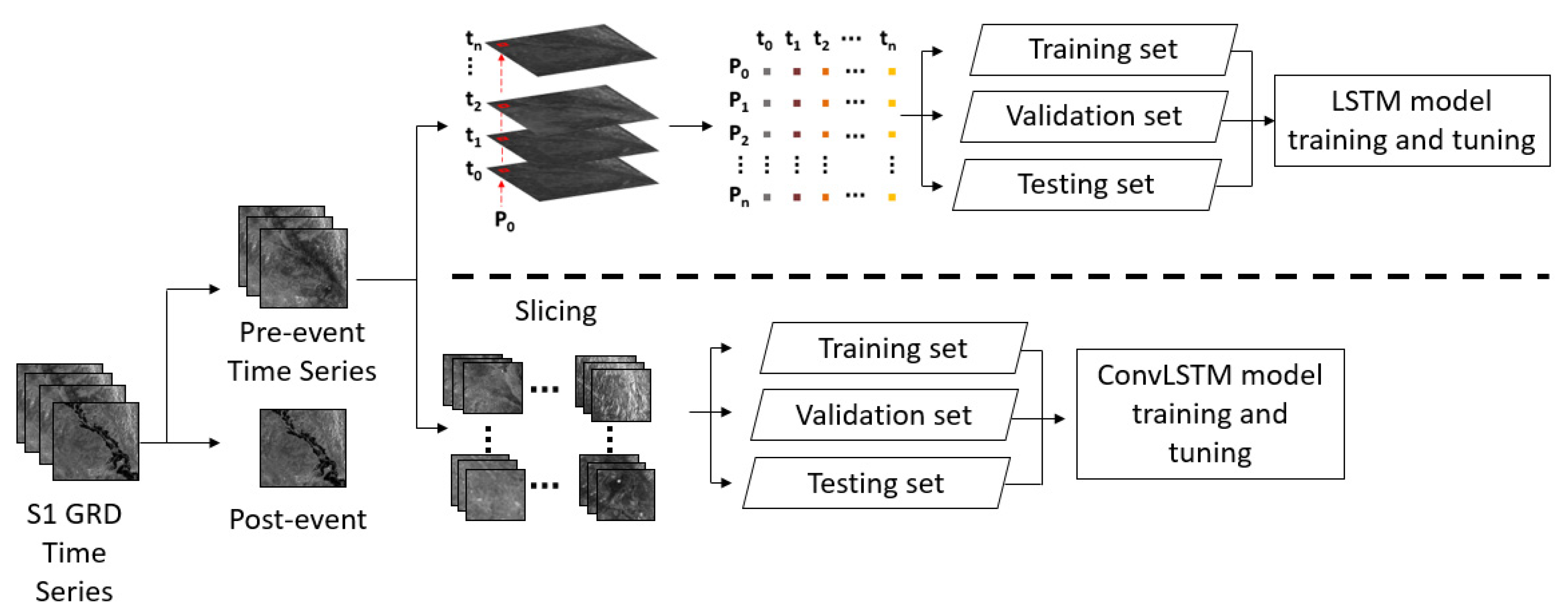
This configuration yields a receptive field of 7: each value in the model’s output has been generated by taking into consideration a region of 7 × 7 pixels from the model’s input [30]. We believe this architecture provides a good balance between representational power (e.g., ability to make predictions in a complex dynamical system) and training time. In each study site, the image stacks were cropped into smaller patches of 50 × 50 to 100 × 100 pixels for Brumadinho and the other sites, respectively; each patch preserved the data across the time domain. Similar to the RNN LSTM model, the data was split using a 70-20–10 training, validation, and testing scheme. The training workflow for RNN LSTM and ConvLSTM models can be seen in Figure 1.
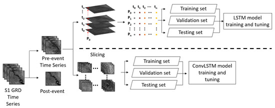
Figure 1.
Processing workflow for the training of RNN LSTM and ConvLSTM models.
In this study, two main reasons justify cropping the arrays into subsets of smaller dimensions. Firstly, enough data was required to train and test the ConvLSTM to spot overfitting or under-fitting. The original Australian training set was composed of 13 images covering an area of around 3588 km2; by dividing the data into smaller patches of 1 km2 we were able to generate 2336 training samples. Secondly, the maximum size of the training batch was limited by the amount of Random Access Memory (RAM) available in the Graphics Processing Unit (GPU); thus, feeding large training batches (i.e., subsets large in the spatial domain and deep in the time dimension) is not recommendable.
2.3. Model Experiment
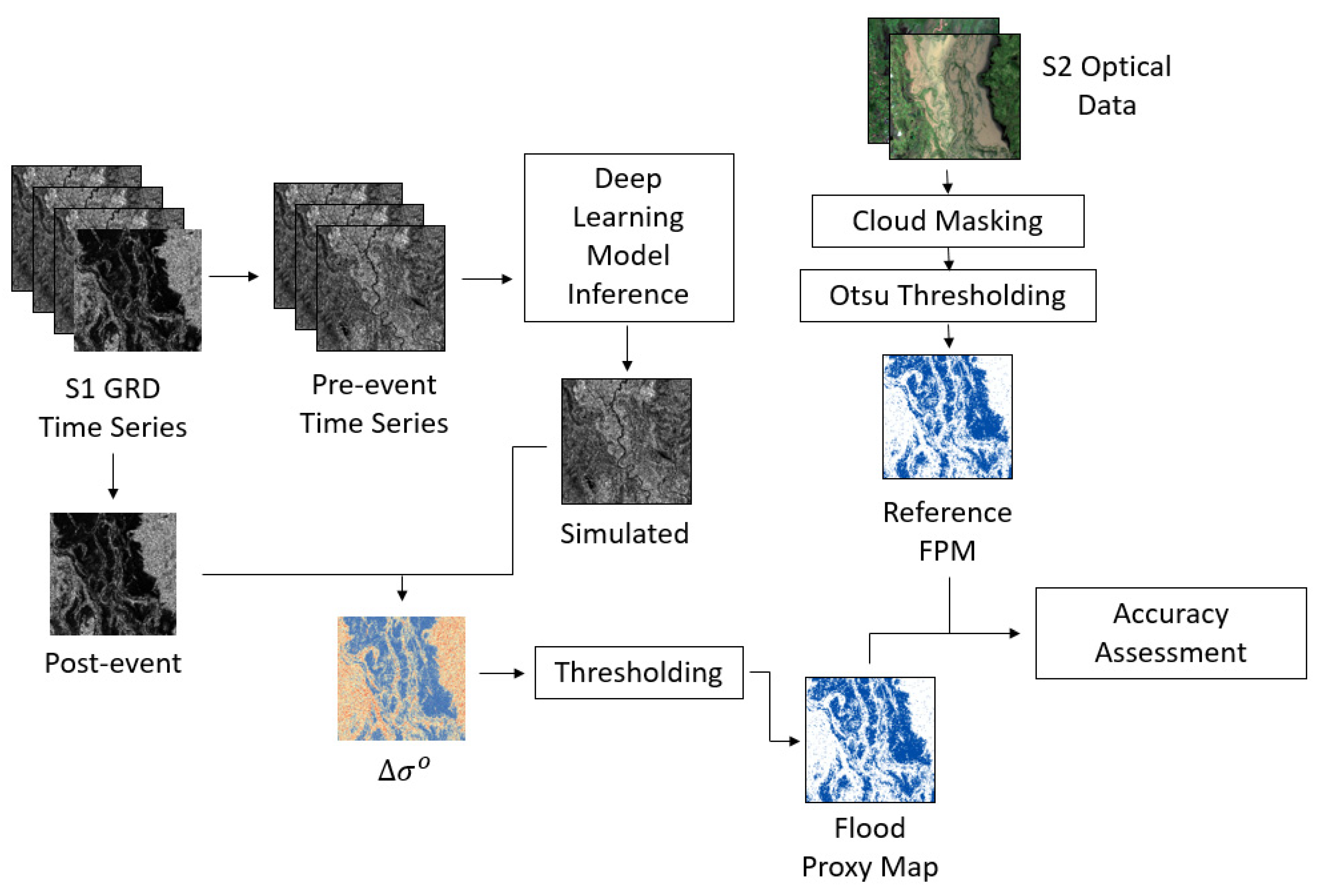
To corroborate the effectiveness of the proposed methods, four different models were examined and compared in this study. Baseline model 1 (B1) uses the last pre-event image before the flood event and Baseline model 2 (B2) uses the historical mean as the pre-event image. The former one is the simplest approach, where the last value of the time series is used. In other words, the last pre-event scene from the stack is compared to the post-event image to construct a Delta image. In model B2, the Delta image is constructed by comparing the per-pixel mean of the whole stack to the post-event scene, since the mean value can be considered as a good estimation of the expected value in the time series. The other two models, the RNN LSTM model (L1) and ConvLSTM model (L2), were designed to generate the synthetic image that was compared with the post-event image in the change detection step (see Figure 2).

Figure 2.
Workflow for the generation of Flood Proxy Maps based on forecasting from RNN LSTM and ConvLSTM models.
Given a stack of S1 images spanning a date range , where the represents the pre-event scene and corresponds to the post-event scene, then the per-pixel Delta for each model is calculated as follows:
The processing, training, and testing of the models were conducted in Google Colab (https://colab.research.google.com/, accessed on 10 July 2020) Pro, a hosted Jupyter notebook service that provides the access to computing resources essential for training deep learning models (i.e., GPUs). The models were written using Tensorflow 2.0 in a Python 3 environment.
3. Study Cases and Data
3.1. Australia—Cyclone Debbie
Tropical Cyclone (TC) Debbie made landfall over Airlie Beach, North Queensland (Figure 3a), on 28 March 2017 at approximately 12:40 p.m. (AEST, UTC + 10:00) as a category 4 storm with winds up to 263 km·h−1 [31]. Strong gusts, extreme precipitation, and slow movement of the system triggered flash and river flooding within the states of Queensland and New South Wales [32]. In some areas of the Fitzroy River basin, the recorded accumulation of precipitation was close to 1000 mm over the two days following the landfall [31]. The estimated economic damage produced by Debbie was 1.7 billion Australian dollars, the second-costliest cyclone in Australia as of 2018 [33], affecting, especially, industries such as farming, mining, and tourism [34].
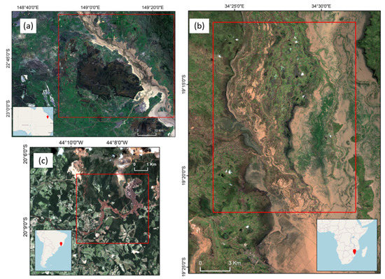
Figure 3.
Sentinel 2 optical data showing the location of the three study sites: (a) Queensland, Australia, (b) Mozambique (b), and (c) Brumadinho, Brazil.
The Area of Interest (AOI) selected for this event encompasses approximately 3588 km2 and is located within the Bowen Basin, between the towns of Middlemount and Clarke Creek, Queensland. It is composed mainly of flat terrains with a gentle slope of less than 5%, and elevation ranging from 90 to 540 m above sea level (mean elevation of 163 m). Soils with low water-holding capacity and high clay content such as kandosols, vertosols, and rudosols are the predominant soil types in the area [35]. In terms of the main types of land use, around 81% of the area is used as grazing native vegetation, 7.5% corresponds to the production of native forest, and 2.6% for irrigated cropping [36].
Both optical and SAR data were acquired within a 5 h window, thus enabling a fair comparison of the flooding extent captured on both datasets. Moreover, the large span of the inundations provided large amounts of data for training and testing deep learning models. Given the aforementioned reasons, we considered Debbie to be a suitable event to compare the performance of different models.
3.2. Mozambique—Cyclone Idai
Cyclone Idai landed as a category 2 storm over the African countries of Malawi, Mozambique, and Zimbabwe (Figure 3b), on 14 March 2019. The winds of up to 175 km·h−1 generated a 4 m tall storm surge around the Pungwe River Delta [37], near Mozambique’s coastal city of Beira, making it one of the most affected locations during this event. Moreover, the provinces of Sofala and Manica were also considerably affected by extreme rainfall as the storm slowly displaced inland. Satellite measurements from NASA’s Global Precipitation Mission (GPM) showed that in some areas of Mozambique the accumulated precipitation over five days exceeded 600 mm [38]. It is estimated that Cyclone Idai occasioned damages upward of 1.4 billion US dollars, whilst affecting 1.8 million people in Mozambique alone, of which 650 were reported dead [39].
In our previous study [40], we focused on this case to develop a texture-based Bayesian probability approach for flood mapping employing the Normalized Difference Sigma-Naught Index (NDSI) and Shannon’s Entropy of NDSI (SNDSI). For this study, we revised this event for two reasons: first, to analyze the consistency in terms of accuracy of LSTM and ConvLSTM models when applied to other extreme weather events on a different geographic region; secondly, to compare such results against a model that do not make use of a deep stack time series data, but rather focus on spatial features. We focused on an area of 276.48 km2, located 65 km northwest of Beira, Mozambique. This AOI is located inside the Pungwe Riven catchment, where the Mean Annual Precipitation (MAP) can reach up to 2020 mm [41]. The site is dominated by herbaceous vegetation (more than 50% of the area corresponding to this type of land cover), with a considerable presence of cultivated vegetation and patches of open forest and shrubs. Soils in the area are classified as clayey-sandy fluvial soils. This site is also characterized by its flat topography, with maximum slopes of 2 degrees.
3.3. Brumadinho
On 25 January 2019, the sudden collapse of the iron ore tailing dam, located inside the Córrego do Feijão mine complex, Brumadinho, Minas Gerais State, Brazil (Figure 3c), released almost 10 million cubic meters of mining waste in less than 5 min [42]. The waves produced in the mudflow reached up to 30 m in height, traveling downhill for as much as 8.5 km until reaching the Paraopeba River [43] and destroying the mine’s administrative center, railway network, and maintenance office along its path. It is estimated that the mudflow affected an area of approximately 3.13 × 10⁶ m2 [44]. Reported on March of 2020, the total number of lives lost is set at 249, while 11 people are still missing. In terms of the number of deaths and volume of waste material released, this incident is considered to be the fifth-largest dam failure in history [45]. This event was selected to explore the applicability of the proposed method on natural disasters other than flooding and its effectiveness over mountainous terrains that pose a challenge to SAR-based change detection methods. The site is located at an altitude of 900 m above sea level, with slopes in the range of 15 to 30 degrees, and with more than 45% covered by closed forest and 25% with open forest.
3.4. Sentinel 1 Image Datasets
Table 1 summarizes the datasets for each study site. For the Australia and Mozambique sites, Sentinel 1 Ground Range Detected (GRD) Sigma naught () data were collected from Google Earth Engine (https://earthengine.google.com, accessed on 12 December 2019). For the Brumadinho site, we acquired Sentinel 1 Gamma naught Radiometric Terrain Corrected () data from the Alaska Satellite Facility (ASF) Vertex Platform (https://search.asf.alaska.edu/, accessed on 20 July 2020). Sentinel 1 RTC products attempt to correct the systematic radiometric effects induced by the terrain, which are more prominent in sites like Brumadinho. The correction is done by normalizing for a local illuminated area projected onto a plane perpendicular to the slant range [46].

Table 1.
Data collected for the three study sites.
3.5. Reference Data
The reference flood masks for Australia and Mozambique study cases were obtained by contrasting pre- and post-event Sentinel 2-derived water masks using the Otsu thresholding method [40]. For the Brumadinho case, the affected zone was manually digitized from 4 m spatial resolution Planet Labs images. Therefore, we must highlight that the accuracy of the flood maps reported in this study is relative to those derived from optical imagery, which we believe represent a good benchmark in the absence of in situ data, but might present any uncertainty inherent from remotely sensed data.
4. Model Application and Assessment
4.1. Threshold Search Grid
Given that the difference in intensity between the simulated and observed images can take either positive or negative values for any pixel, we simultaneously applied positive and negative thresholds to capture areas over which discrepancies are more significant.
A grid search was carried out to try out different combinations of pairwise thresholds. At each iteration, pixels with values higher than the positive threshold were labeled as the flood-affected zone; conversely, those with values below the negative threshold were also labeled as such. Subsequently, the resulting flood maps were compared to the reference flood map to construct a confusion matrix. We evaluated the performance of the models based on the following metrics derived from the confusion matrix:
Recall
Represents the fraction of correctly detected positive events calculated by:
where , , and represent True, False, Positive, and Negative, respectively.
Precision
The fraction of true positive samples between the samples classified as positive by the model:
F1 Score
The Score [47] can be seen as the harmonic mean of the precision and recall, where both of those metrics have an equal relative contribution.
Critical Score Index
The Critical Score Index (), also known as the threat score, represents the ratio between correctly predicted observed positive observations and total positive observations. It is seen as a metric that evaluates the detection accuracy when the amount of True Negatives samples is larger than the others.
Cohen’s Kappa
Cohen’s Kappa () [48] is a statistic that assesses the level of agreement between two classifiers on a classification problem. It is calculated using:
where represents the overall accuracy and is the probability of random agreement found by:
Cohen’s Kappa () can range from −1 to +1, where a value of 1 means the agreement between the classifiers is perfect and a value of 0 indicates an agreement expected from random chance.
4.2. Multi Threshold Approach
The applicability of the thresholds determined from the Australia case was examined on the Mozambique dataset, based on the premise that global thresholds for flood delineation derived on one case can also be applied to other regions as long as the topographic conditions and land cover present a certain degree of similarity. We selected 10 pairs of negative and positive thresholds with the highest Kappa on the TC Debbie scenario, and, with each pair, we created a binary flood map for Cyclone Idai. Furthermore, we stacked the 10 FPMs and counted the frequency in which each pixel was detected as flooded, and present it as relative frequency. Such results can be interpreted as an initial estimation of the flood extent and can be further improved on as more knowledge of the situation and local conditions are obtained.
5. Results and Discussion
5.1. Convolutional LSTM
5.1.1. Validation of Prediction
We assumed that the ConvLSTM model was capable of identifying the spatiotemporal patterns within the data and consequently making an accurate prediction of the next value in the time series. To confirm the forecasting capabilities of the ConvLSTM architecture, we trained and tested ConvLSTM models using a dataset from the Australia site with no flooded scenes. This setup used 21 S1 scenes acquired after Cyclone Debbie, from 4 April to 8 December for model training. The predicted image was then compared to the scene acquired on 22 December. Results of the experiment can be seen in Figure 4 and Figure 5. For VV polarization, the mean value of the Delta image was 0.31 dB (SD = 1.433, RMSE = 1.466); this was slightly better than those for the VH channel (M = 0.799, SD = 1.715, RMSE = 1.892).
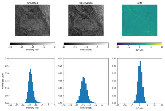
Figure 4.
Simulated, real observation and Delta image with their respective histograms for VV polarization. Real observation corresponds to 20 December 2017.
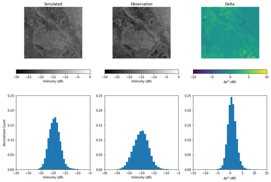
Figure 5.
Simulated, real observation and delta image with their respective histograms for VH polarization. Real observation corresponds to 20 December 2017.
From the histograms, we observed the radiometric similarities between the forecasted and observed S1 images. It can also be seen that the distribution of Delta values corresponded to a normal distribution centered around 0 ± 0.5 dB. Lower Delta values highlighted a good agreement between prediction and observation, and thus it showcases that the ConvLSTM model, thanks to the use of convolutional filters in input-to-state and state-to-state transitions, can effectively leverage the spatiotemporal patterns to predict the next scene in the S1 time series.
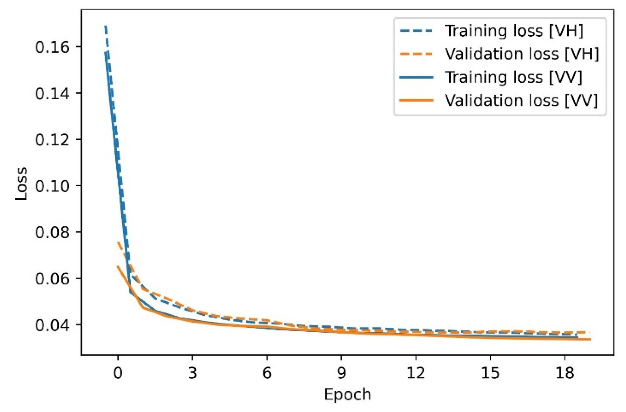
As we can see from the learning curves of the loss function (Figure 6), the training loss and validation loss steadily decrease after a few epochs and reach a plateau after 15 epochs or so. Moreover, the validation curves and training curves are close to one another, meaning that the model is not overfitting too much and has good generalization capabilities.

Figure 6.
Mean Squared Error loss over iterations (Epochs) for ConvLSTM model.
After confirming the prediction capabilities of our spatiotemporal deep-learning framework, we examined flood events in three study sites: Australia, Mozambique, and Brumadinho. The analysis involved the generation of Delta images, thresholding using Delta histograms, deriving heatmaps for different accuracy metrics, and the flooded zone delineation.
5.1.2. Australia Flooding (Cyclone Debbie)
From Figure 7, we observed that the main discrepancies between the target image and the prediction corresponded to the inundated zones. Those areas represent outlier values in the time series that the model has never seen during training, and therefore is unable to forecast. If we compared the statistics of the Delta images (Table 2), we can see that when the target image captures a flooding event there is higher disagreement with the prediction, proven by a higher mean, root mean square error, and standard deviation.
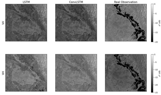
Figure 7.
Images predicted by RNN LSTM (L1) and ConvLSTM (L2) models. Real observation corresponds to 31 March 2017.
Table 2.
Statistics of Delta images for Australia site.
Therefore, we can delineate the flooded areas through thresholding of the difference between the prediction and the real observation. In this case, we applied positive and negative thresholds in increments of ±0.25 dB to the Delta image, and the resulting Flood Proxy Map was compared against the reference. Results from the accuracy assessment for all the models used in the cyclone Debbie case can be seen in Figure 8.
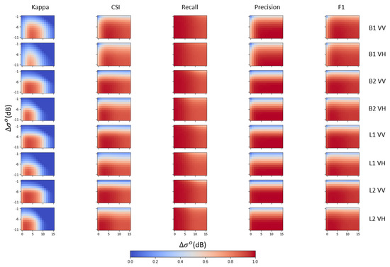
Figure 8.
Heat maps for Kappa, Critical Score, Recall, Precision, and F1-Score for all models tested in the Cyclone Debbie (Australia) case.
The results of the accuracy assessment show that all models, in general, were capable of achieving relatively high F1 and CSI scores, thanks to the high precision and recall values (see Table 3). From the metrics implemented, we found Cohen’s Kappa to be more sensitive to threshold changes. For this reason, we decided to use Kappa as a metric of model performance in the two other study sites.
Table 3.
Maximum value for the metrics used in the accuracy assessment.
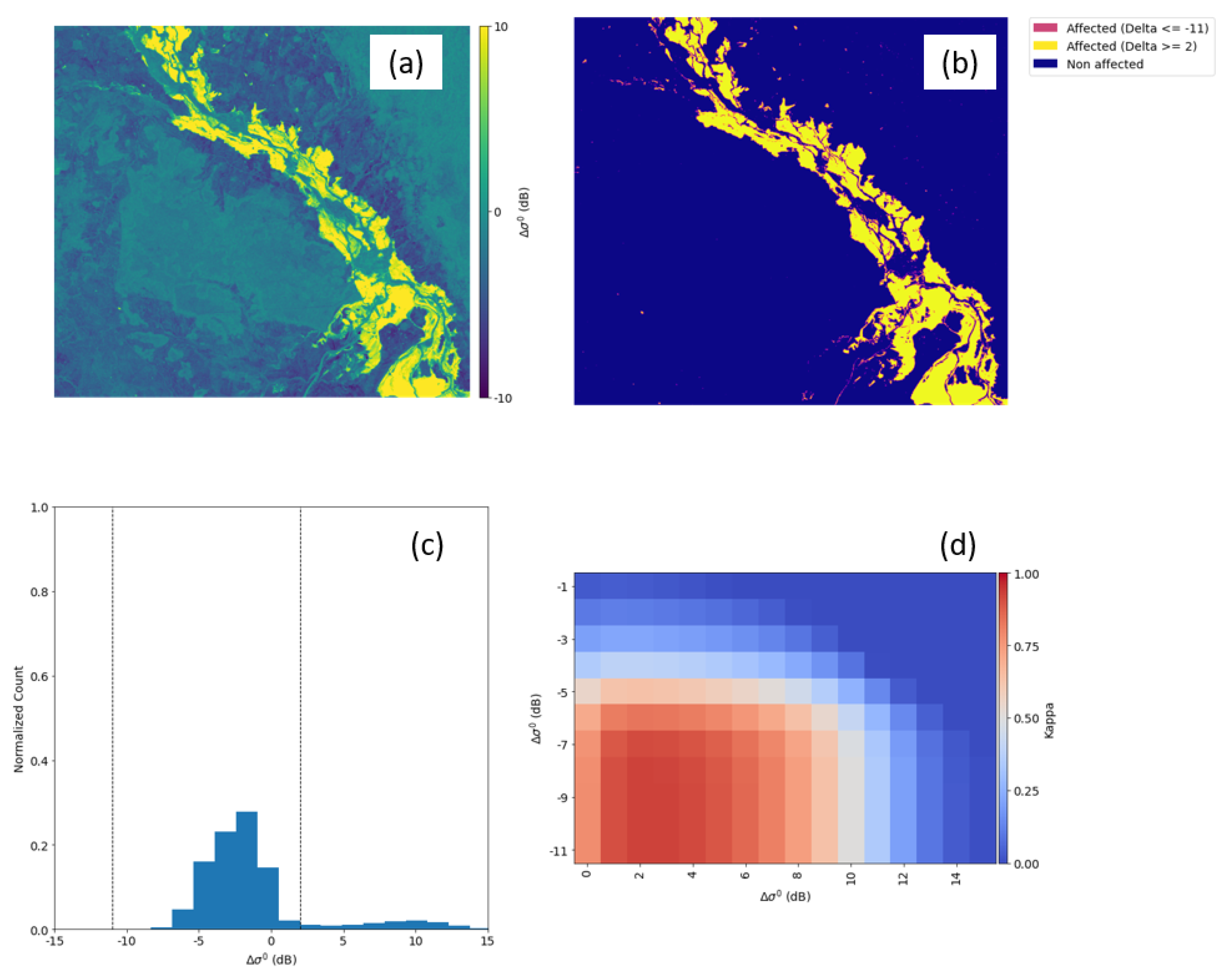
In Figure 9a, a clear distinction between flooded and non-flooded areas in the Delta () image can be observed. Bright areas represent pixels with a high Delta, mainly caused by the loss of backscattering in the during-flood image. In open-water flooding, the electromagnetic signal of the SAR satellite bounces away from the sensor when hitting the water’s surface (specular reflection), assuming there is no influence of the wind and capillary waves. Moreover, the large extent of the flooding for this case points to a large presence of pixels with high Delta, and the delineated flood-affected zone is shown in Figure 9b.
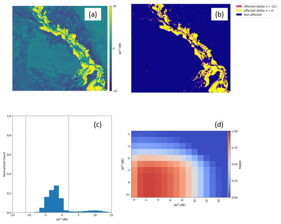
Figure 9.
Australia ConvLSTM Delta image of VV polarization (a), Flood Proxy Map (b), Histogram of Delta image (c), and Cohen’s Kappa heatmap (d).
In Figure 9c, two populations of can be observed: one centered around of −1.5 dB, and another centered at of 10 dB. We expected that the population of open-water flooding pixels corresponded to the second population at the right of the histogram, where is higher. The Cohen’s Kappa heat map generated in the threshold grid search for VV polarization is shown in Figure 9d. Values in the X-axis are the positive Delta thresholds, and Y-axis is the negative thresholds. This heat map shows threshold combinations with high classification accuracy (i.e., high Kappa) in red and those with low accuracy in blue. As seen on the heat map, the highest accuracy was achieved when using positive around 2 or 3 dB, and negative in the range −7 to −11. We applied the pair ≥ 2 and ≤ −11 (dash line in Figure 9c) to generate the FPM (Figure 9b), where it is visible that most of the pixels labeled as flooded are those detected by the positive threshold (displayed in yellow).
Additionally, it is important to mention that the Kappa heat map also indicates that the FPM is more sensitive to positive thresholds, in the sense that the variations of Kappa along the horizontal axis are higher than on the vertical axis, mainly because most of the flooding was open-water. Some inundated urban areas within the boundaries can also be observed, where double-bouncing may take place, that contributes pixels with negative values.
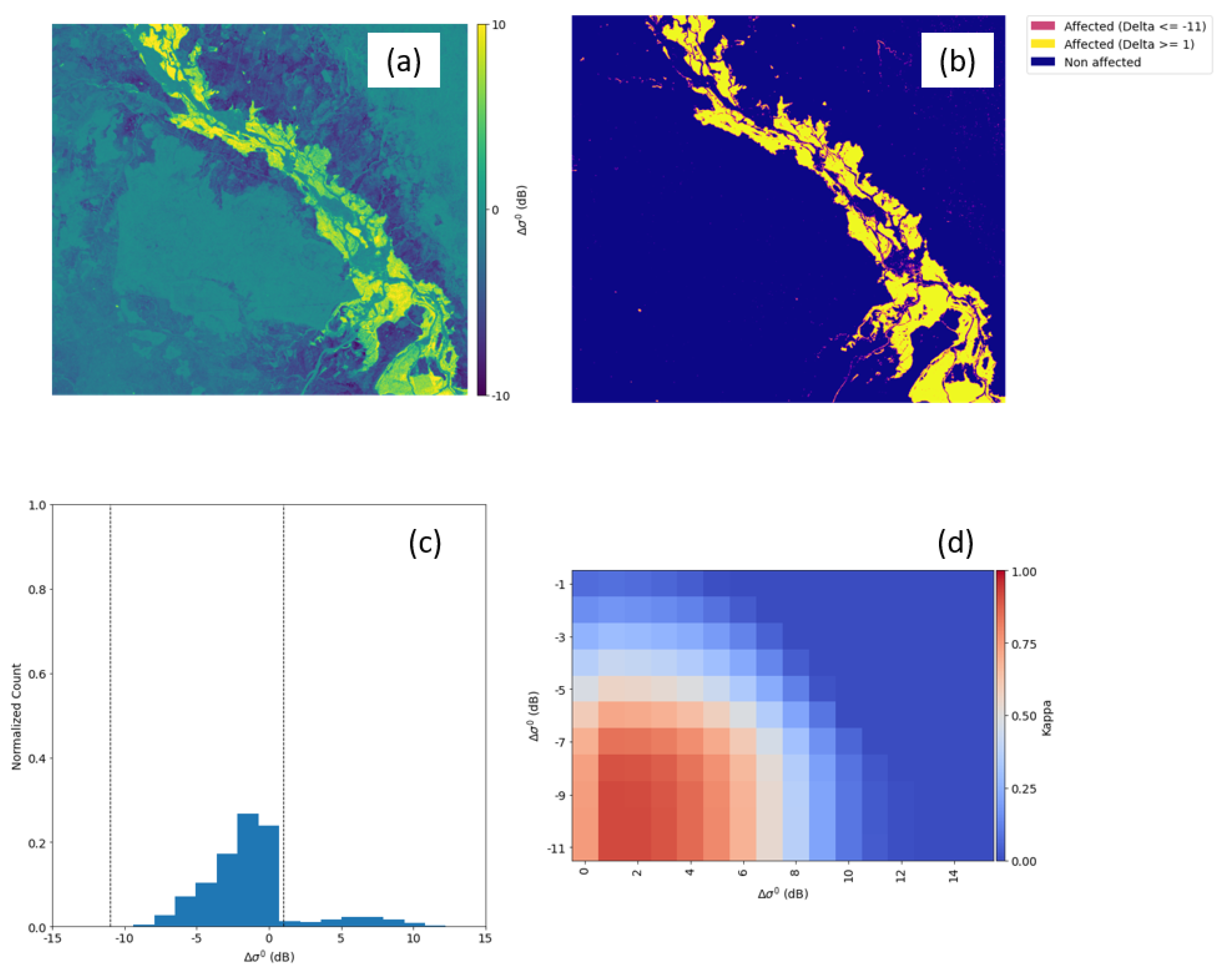
In Figure 10, it can be observed that similar results were obtained for VH polarization data. The spatial distribution of pixels with high Delta followed a similar pattern as in the VV polarization. In terms of thresholding selection, we can also appreciate more sensitivity, accuracy-wise, for positive values than for negative ones, as in the VV polarization dataset.
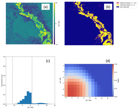
Figure 10.
Australia ConvLSTM Delta image of VH polarization (a), Flood Proxy Map (b), Histogram of Delta image (c), and Cohen’s Kappa heatmap (d).
In terms of error types, we observed that our change detection method based on ConvLSTM (L2) predictions was prone to overestimate the extent of the inundated area (i.e., higher commission error). The total area of false positives was 72.6% larger than false negatives for the VV channel, and 48% higher for VH. The resulting FPM for VV and VH polarizations are shown in Figure 11.
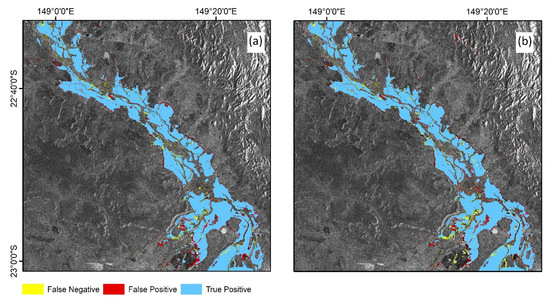
Figure 11.
Flood Proxy Maps from ConvLSTM model with classification errors for VV polarization (a) and VH polarization (b).
We further examined the errors of the ConvLSTM model according to land cover types extracted from the 2017 Copernicus Global Land Cover Layer created by European Space Agency (ESA) [49]. From Table 4 we can observe that the main source of error belonged to areas covered by herbaceous vegetation, open forest, or closed forest, further corroborating the fact that using C-band for flood mapping over vegetated areas remains a challenging task [50,51,52,53].
Table 4.
L2 model error sources per Land Cover type (km2).
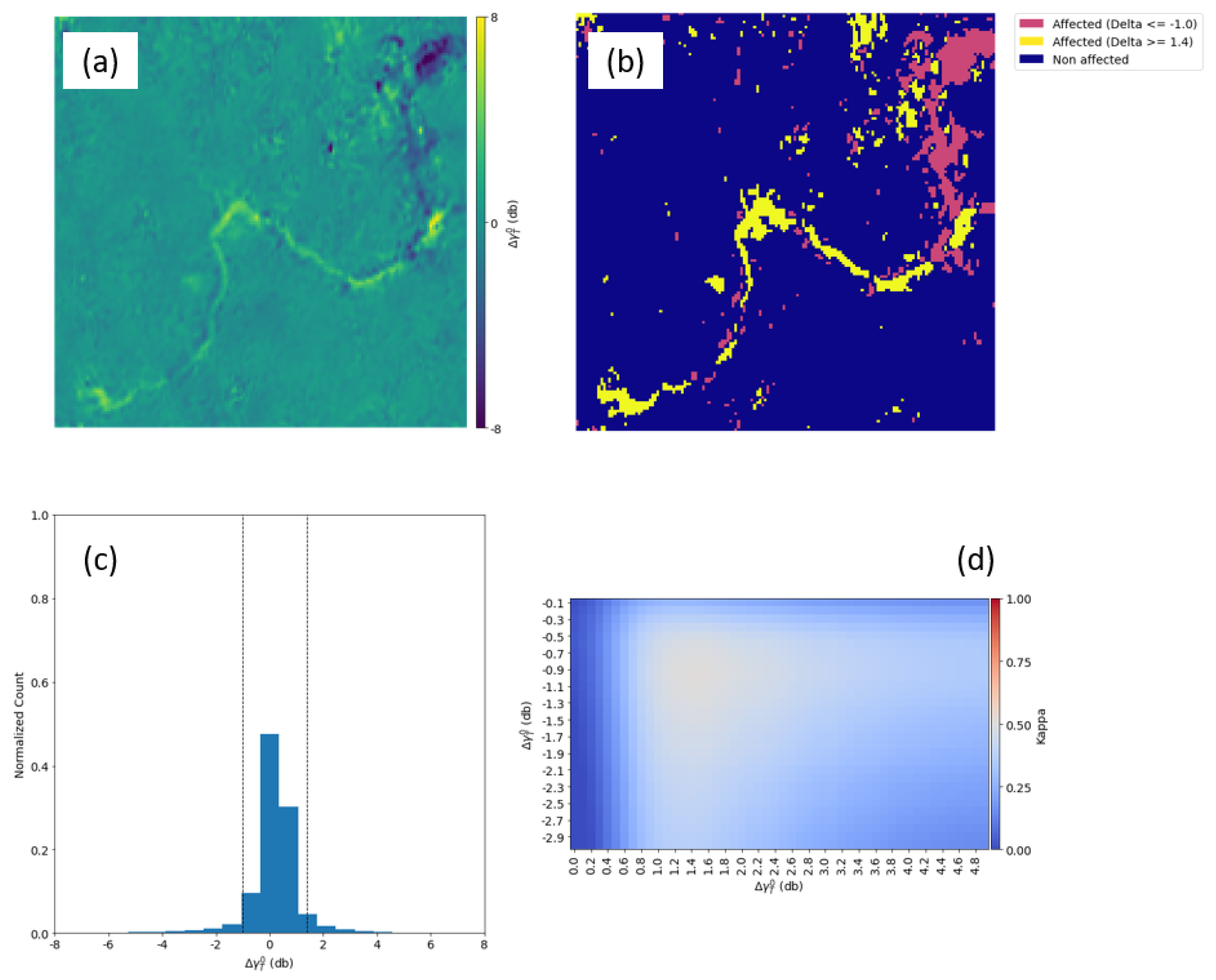
5.1.3. Mozambique Flooding (Cyclone Idai)
For this event, the synthetic backscattering values were close to the real observations by ±1 dB, as shown by the Delta products’ histograms in Figure 12c (VV polarization) and Figure 13c (VH polarization). However, the distinction between inundated and dry areas in terms of values was not as clear as it was in the previous case. One possible explanation is that the Mozambique site is a more dynamic landscape due to the land cover types (e.g., crops), whose higher degree of variability across time makes it even more challenging to correctly forecast the next value in the time series. Additionally, in this proposed framework, we assumed that the biggest Delta values fell on flood-affected zones; however, it is very likely that land cover changes not associated with flooding were responsible for the significant disagreement between prediction and observation. One must be aware that the probability of detecting such changes increases in dynamic sites with high heterogeneity.
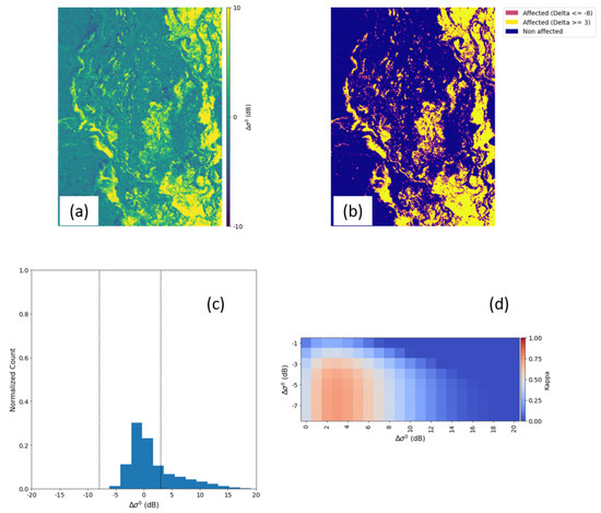
Figure 12.
Mozambique ConvLSTM Delta image of VV polarization (a), Flood Proxy Map (b), Histogram of Delta image (c), and Cohen’s Kappa heatmap (d).

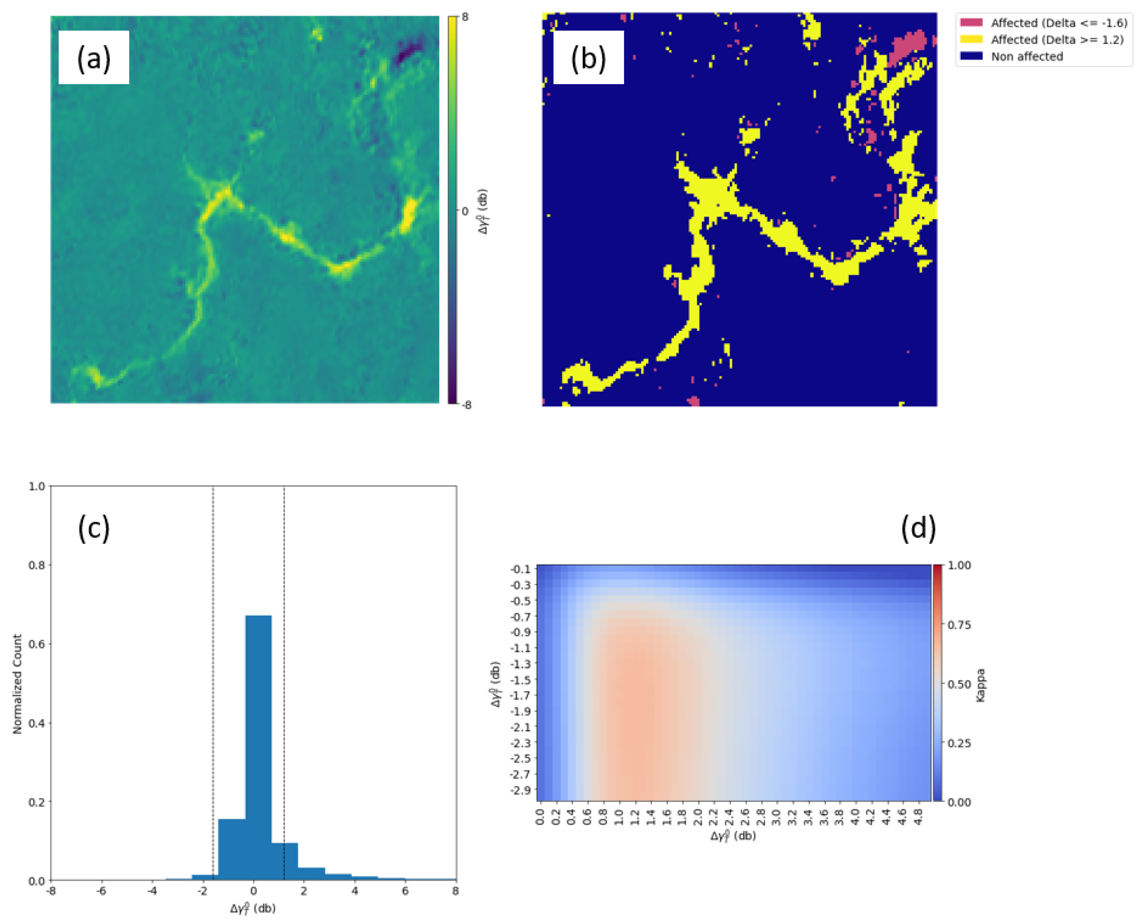
Figure 13.
Mozambique ConvLSTM Delta image of VH polarization (a), Flood Proxy Map (b), Histogram of Delta image (c), and Cohen’s Kappa heatmap (d).
5.1.4. Brumadinho
The mapping of the mudslide event triggered by the dam failure in Brumadinho represented the most challenging case in this study. The release of huge amounts of sludge downstream occasioned several changes to the terrain, which we tried to map all at once, including damage to infrastructure, riverside bank erosion, and flooding.
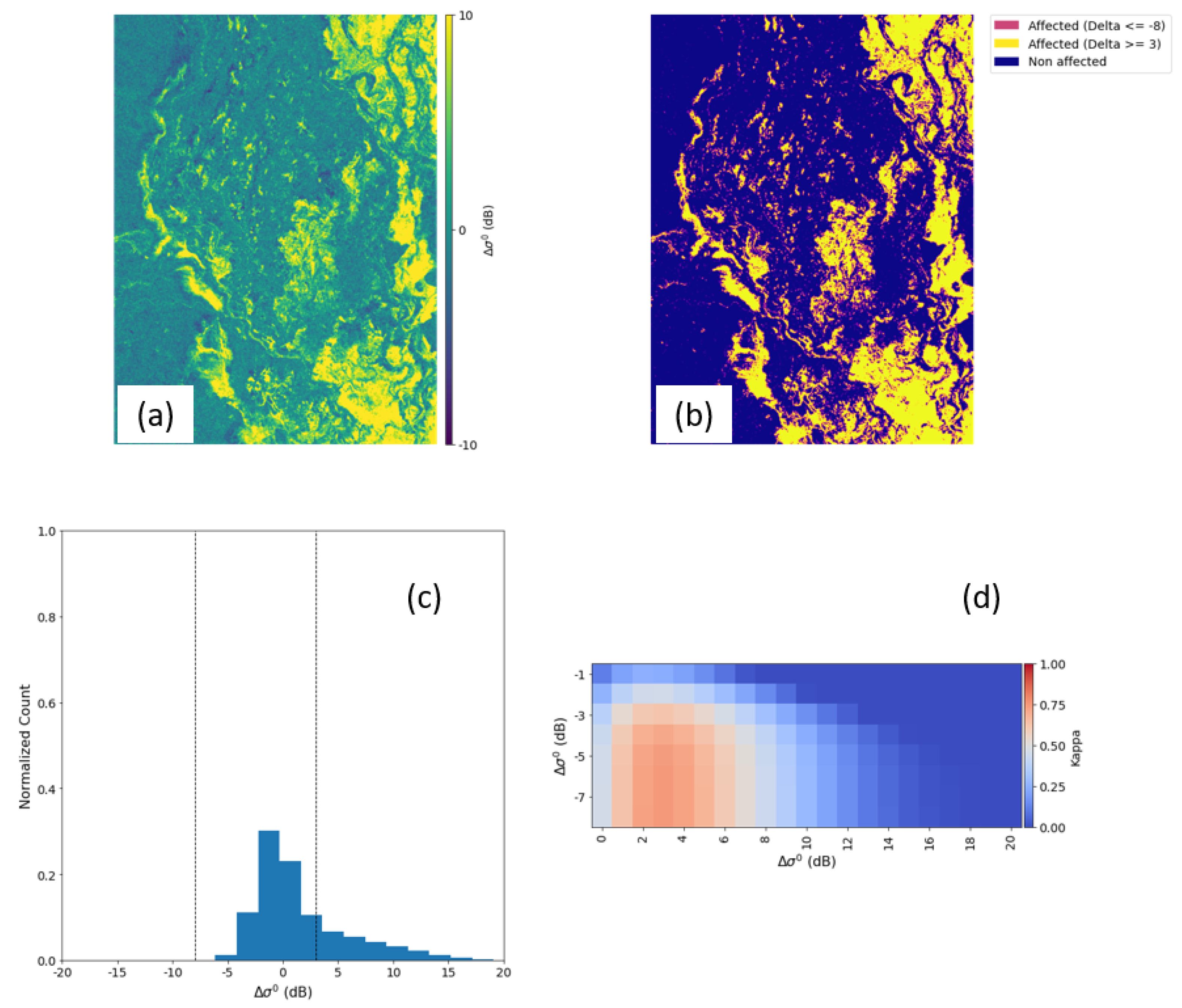
In Figure 14, most of the damage along the riverbank was enhanced, as well as the changes that took place upstream, where the rupture took place, and the mapping accuracy achieved by this method when analyzing the VV polarization dataset was suboptimal. The changes to topography that took place in the site where the reservoir was located are visible in the upper right part of the product (Figure 14a). The transformation from a flat surface to a hilly topography resulted in a substantial increase in the strength of the return signal, hence the lower value. Moreover, quite the opposite took place when the mud wave cleared the vegetation present at the riverside as it flowed downstream, creating a bare surface once it settled down. The mapping accuracy of the ConvLSTM method yielded the highest Kappa of 0.51 for the VV dataset (Figure 14d) and 0.66 for the VH dataset (Figure 15d), which was slightly better than a random classification.
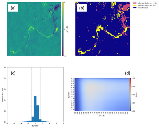
Figure 14.
Brumadinho ConvLSTM Delta image of VV polarization (a), Flood Proxy Map (b), Histogram of Delta image (c), and Cohen’s Kappa heatmap (d).
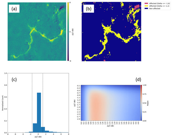
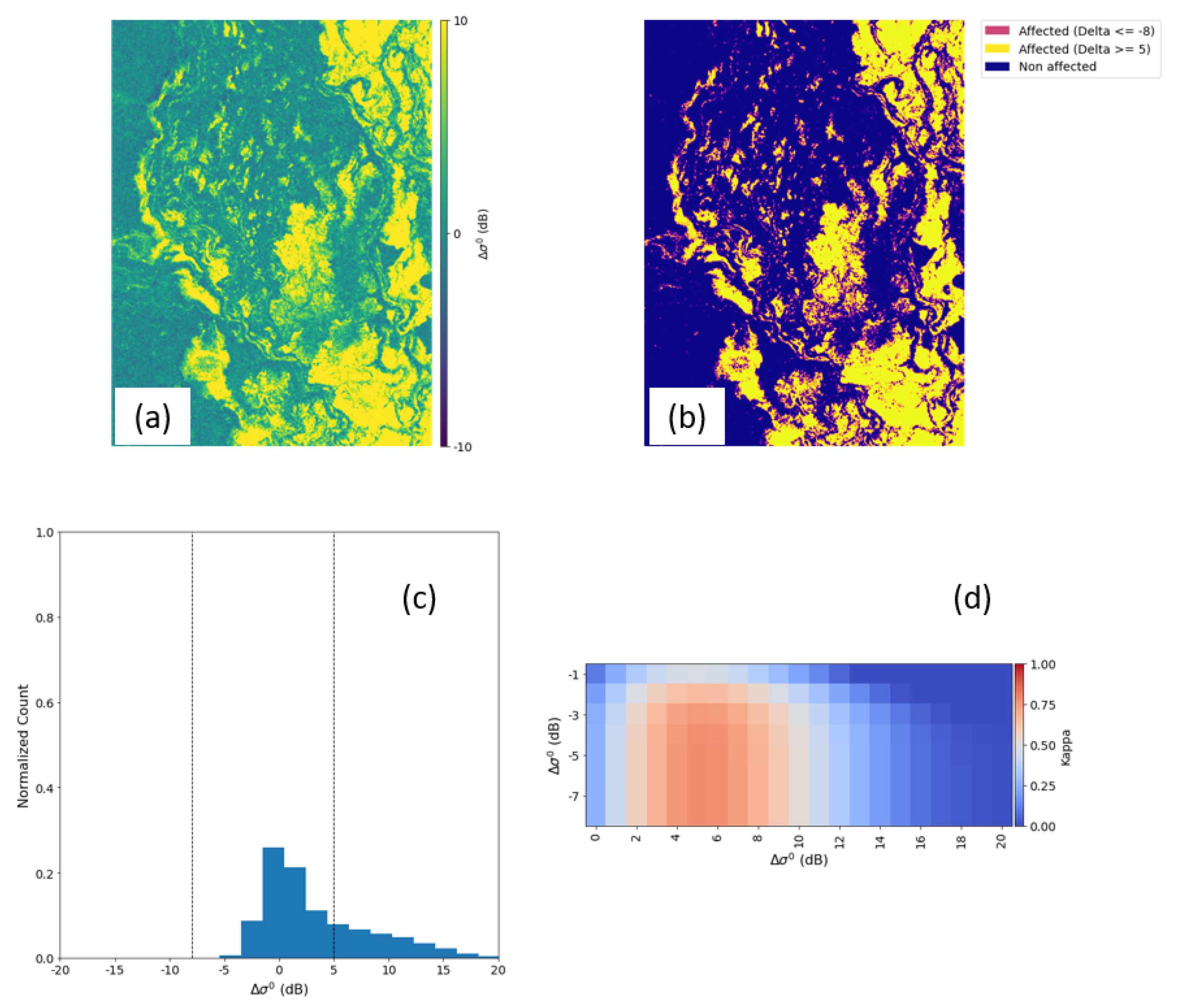
Figure 15.
Brumadinho ConvLSTM Delta image of VH polarization (a), Flood Proxy Map (b), Histogram of Delta image (c), and Cohen’s Kappa heatmap (d).
A higher Kappa value of the FPM was obtained with VH polarization. The best results were derived by the ConvLSTM products when the thresholds ≥ 1.2 dB and ≤ −1.6 dB were set, achieving a Kappa of 0.66.
5.2. Model Comparison
Table 5 summarizes the flood mapping accuracies (Kappa) of the four tested models in the three study sites. Overall, we obtained classification Kappa values above 0.72 from the L1 and L2 models in Australia and Mozambique.
Table 5.
Summary of Kappa values obtained in the three study sites.
In the Australia study site, the four models were compared. The simple change detection, B1, achieves Kappa values of 0.87 and 0.75 for VV and VH polarizations, respectively. For B2, using the mean of the stack in the Delta calculation further improved the results in both polarizations with Kappa of 0.91 and 0.87. Furthermore, the L1 model slightly improved the accuracy of the VH dataset with a Kappa of 0.89. Finally, the L2 model outperformed all the models with Kappa of 0.93 for VV and 0.92 in VH datasets.
When focusing on the application of L1 and L2 models in Australia and Mozambique study sites, as expected, the use of spatiotemporal features advanced the performance of the ConvLSTM. Unlike the LSTM model, in which all spatial correlation is lost due to the unraveling of the arrays into a 1-D vector, the implementation of a convolutional kernel in the ConvLSTM makes the model take advantage of the spatial correlation of adjacent pixels. Also, in Mozambique, our results from the LSTM and ConvLSTM models were able to outperform the accuracy of flood mapping from our previous study, using the Entropy NDSI method [40], indicating that the LSTM-based thresholding method was able to enhance the classification accuracy in both VV and VH datasets.
In the Brumadinho study site, the mapping accuracies were just slightly better than a random classification. We considered that factors such as spatial scale, topography, and land cover may have all affected the performance of the models.
In terms of spatial scale, the Brumadinho site was the smallest of the sites explored in this study; it is 150 times smaller than the Australia site, and about 14 times smaller than Mozambique. This could be an indication that the area analyzed in Brazil may not be large enough for the ConvLSTM architecture to properly model such a dynamic and complex landscape, since a smaller coverage translates to a lower number of training samples. Lower performance can also be linked to the rugged topography of the site, with slopes between 15 to 30 degrees, which consequently causes artifacts on the SAR intensity images (i.e., layover and shadow effect), depending on the orbit and viewing geometry during data acquisition. Additionally, the abundant forest cover of the site makes it difficult to detect land-cover changes using basic intensity-based change detection methods. The dynamic nature of the forest area makes the backscattering values over the same area constantly vary as leaves’ dielectric properties (i.e., higher after rain), canopy growth and other conditions determine how the radar signal interacts with the vegetation. However, for model comparison, the best results were derived by the ConvLSTM products achieving a Kappa of 0.66, showing an improvement of almost 10% when compared to the baseline models, and 5% to LSTM.
These results indicate the feasibility of the proposed ConvLSTM to produce damage maps for different and more complicated cases other than open-water flooding over floodplains. Also, in our case study, the VH polarization datasets constantly produced better results, although the decision of which polarization works best seems to be case-dependent, as the local conditions and damages to be mapped differ from zone to zone. However, the VH-polarized data is suggested to generate preliminary FPM for an emergent case, as it has shown to produce satisfactory results overall in this study.
5.3. Application of Multi-Threshold for Flood Mapping
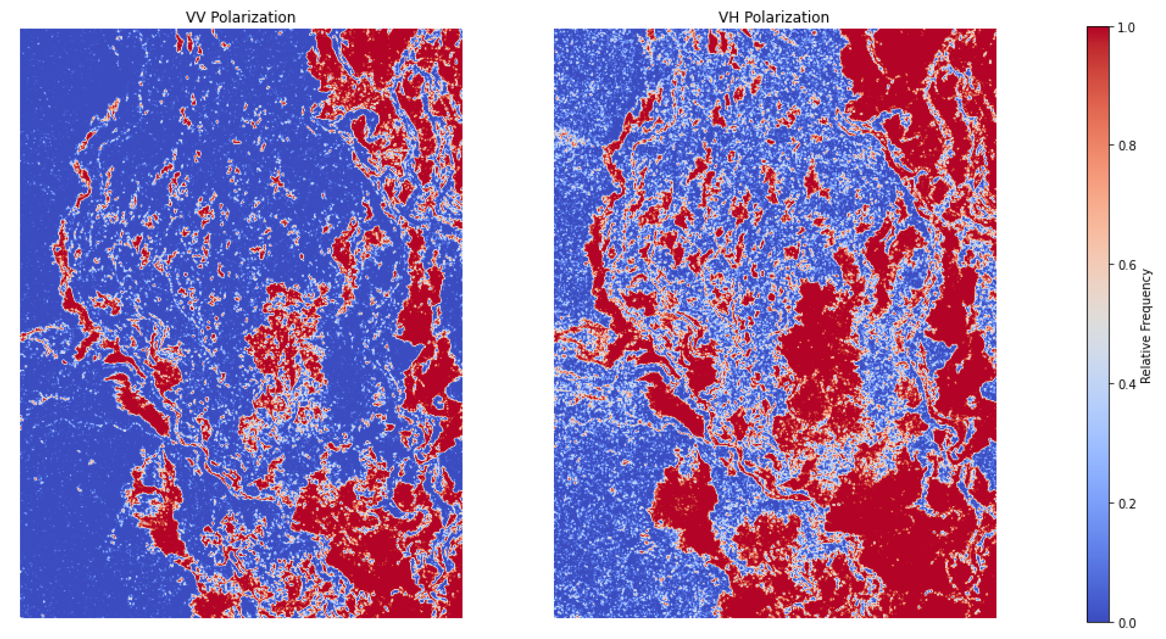
The thresholds determined from the Australia case were tested in the Mozambique dataset. Pairs of negative and positive thresholds with the highest 10 Kappa values extracted from the TC Debbie event were used to create 10 binary FPMs for Cyclone Idai. Furthermore, by combining the 10 FPMs and counting the frequency of floods in each pixel, the relative frequency/probability map can be produced to represent the likelihood of flood occurrence.
The results from the multi-threshold approach are shown in Figure 16, using the Mozambique flood as an example. The values in the final product ranged from zero to one. A value of zero represents a pixel that was not considered as inundated in any of the 10 iterations; conversely, a value of one means a flooded pixel under all the thresholds applied.
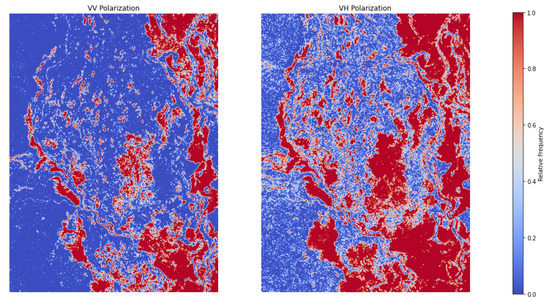
Figure 16.
Mozambique Flood Relative Frequency for VV polarization (left) and VH polarization (right).
These products were then tested to perform a binary classification to generate FPM, using 0.5 and 0.9 as cut values. Under these settings, the Kappa coefficient for the VH polarization was 0.58 and 0.69, respectively. On the other hand, VV polarization achieved accuracies of Kappa 0.75 and 0.73.
For the VH-polarized product, the performance dropped significantly when a 50% relative frequency was used as a threshold, as a consequence of a larger commission error. When a more conservative cut value was selected, the results were more in line with those obtained in the threshold grid search.
If we solely focus on VV polarization, it is fair to say that this method can be replicated in future flooding cases to generate preliminary flood extent maps that can provide a first glance at the magnitude of the flooding, information that could be crucial for local stakeholders who perform disaster relief tasks. Nonetheless, the same cannot be said of the VH polarization. To further understand the factors that contributed to such a significant gap in performance across the two polarizations, it may be helpful to take a look at the principal land cover types of the sites.
5.4. Potential Effect of Land Cover on Model Application
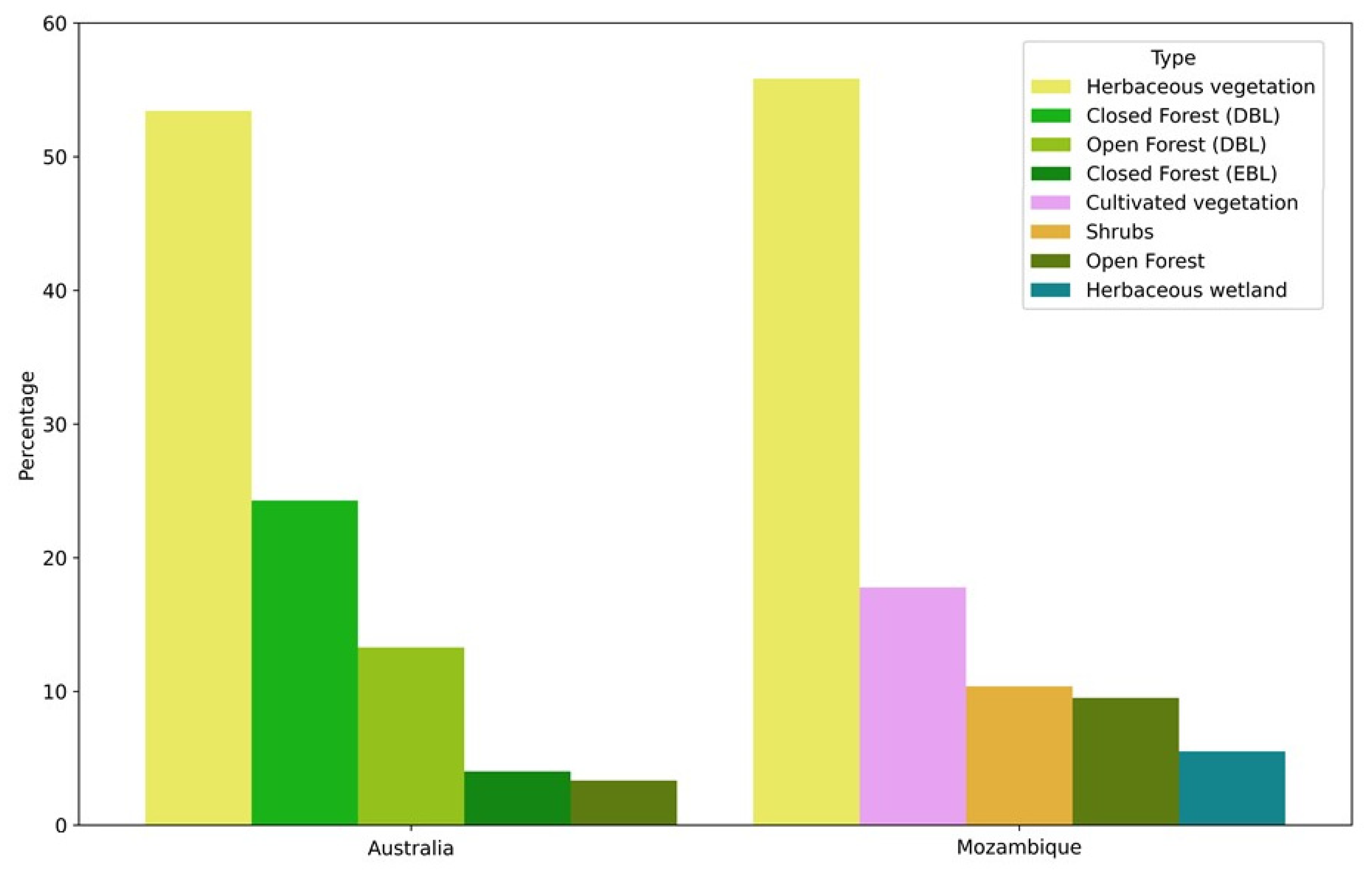
Table 5 shows that both L1 and L2 significantly outperformed in Australia than in Mozambique. A potential factor that leads to this difference could be subject to the characteristics of the land surface in the two study sites. Figure 17 shows the five principal land cover types that make up more than 95% of the sites of Australia and Mozambique, provided by the Copernicus Global Land Cover Layer [49]. Herbaceous vegetation represented the major class as it covered more than 50% of the area in both sites. The study scene in Australia is characterized by the presence of open and closed broadleaf forests, whereas the Mozambique site shows a considerable presence of cultivated vegetation and woody perennial plants (shrubs).

Figure 17.
Percentage of area for each of the mainland cover types for Australia and Mozambique sites.
The difference in the types of vegetation present in the two areas can account for the dissimilarity in performance when applying the thresholds of the Australia site to the Mozambique dataset. We suggest the cross-polarization (VH) is more susceptible to volumetric scattering mechanisms generated from canopy or trunks of vegetation; as a result, the thresholds used in one area would need to be reassessed when utilized on another if the land cover characteristics are not similar, as in this scenario.
6. Conclusions
In this study, we have proposed a method for employing deep learning-based time series analysis for Flood Proxy Mapping generation. Long Short-Term Memory and Convolutional LSTM models are capable of properly simulating a synthetic pre-event image in a Sentinel One intensity time series. The predicted images can subsequently be compared to the post-event image to identify flooded areas where simulated and observed values disagree significantly.
In the Australia case, LSTM and ConvLSTM models produced FPMs with the highest classification accuracy when compared to the baseline models. The Cohen’s Kappa coefficient for the latter were 0.93 and 0.92, for VV and VH polarization, respectively. Similarly, ConvLSTM outperformed the rest of the models in our Mozambique dataset in both polarizations, achieving Kappa values of 0.75 (VV) and 0.78 (VH). In the Brumadinho site, the obtained results show lower accuracies across all models, which could be subjective to the effect of hilly terrains. However, ConvLSTM was still able to generate moderately good results (Kappa of 0.66) when the VH-polarized dataset was used, showing the applicability of our proposed method in areas where traditional SAR-based change detection methods struggle, such as mountainous and vegetated areas. These results demonstrate the performance boost that convolutional operations provide in time series analysis of satellite data incorporating spatial-related features.
The pre-calibrated Delta thresholds can be effectively applied to map inundated areas across different study sites. By applying the 10 most effective thresholds of the Australia case onto the Mozambique case, we were able to generate a map of the relative frequency of flood pixels. When relative frequency cut values of 0.5 and 0.9 were selected, Kappa values of 0.75 and 0.73 were obtained in VV data, respectively.
Potential future applications of the ConvLSTM Delta approach include the implementation of the model in the same site to delineate historic flooding events and subsequently generate a baseline of flooded areas and their corresponding returning periods. Additionally, by applying the multi-threshold approach on a larger number of sites and flooding events, we could potentially uncover guiding physical–mathematical–statistical rules that may lead to establishing potential global thresholds for flooding detection in different regions worldwide.
Finally, the length or range necessary to stochastically model the spatiotemporal behavior of a random variable is quite important in the domain of frequency, space, or time. Therefore, further studies could be conducted to evaluate the correlation between the depth of stack and model performance.
Author Contributions
Conceptualization, N.I.U., S.-H.Y. and S.-H.C.; Formal analysis, N.I.U.; Methodology, N.I.U., S.-H.Y. and S.-H.C.; Software, N.I.U.; Supervision, S.-H.Y. and S.-H.C.; Writing—original draft, N.I.U.; Writing—review & editing, S.-H.Y., S.-H.C. and R.F. All authors have read and agreed to the published version of the manuscript.
Funding
Part of this research was carried out at the Earth Observatory of Singapore via its funding from the Nanyang Technological University Award #021255-00001 (EOS Contribution Number 413), SWCB-110-051, and MOST 110-2121-M-008-003.
Conflicts of Interest
The authors declare no conflict of interest.
References
- Raadgever, T.; Hegger, D. Flood Risk Management and Strategies and Governance; Springer International: Cham, Switzerland, 2019. [Google Scholar]
- Schumann, G.J.P.; Moller, D.K. Microwave remote sensing of flood inundation. Phys. Chem. Earth Parts A/B/C 2015, 83–84, 84–95. [Google Scholar] [CrossRef]
- Amarasinghe, U.; Amarnath, G.; Alahacoon, N.; Ghosh, S. How Do Floods and Drought Impact Economic Growth and Human Development at the Sub-National Level in India? Climate 2020, 8, 123. [Google Scholar] [CrossRef]
- Miller, J.D.; Hutchins, M. The impacts of urbanisation and climate change on urban flooding and urban water quality: A review of the evidence concerning the United Kingdom. J. Hydrol. Reg. Stud. 2017, 12, 345–362. [Google Scholar] [CrossRef] [Green Version]
- Kundzewicz, Z.; Kanae, S.; Seneviratne, S.; Handmer, J.; Nicholls, N.; Peduzzi, P.; Mechler, R.; Bouwer, L.M.; Arnell, N.; Mach, K.; et al. Flood risk and climate change: Global and regional perspectives. Hydrol. Sci. J. 2014, 59, 1–28. [Google Scholar] [CrossRef] [Green Version]
- Hirabayashi, Y.; Mahendran, R.; Koirala, S.; Konoshima, L.; Yamazaki, D.; Watanabe, S.; Kim, H.; Kanae, S. Global flood risk under climate change. Nat. Clim. Change 2013, 3, 816–821. [Google Scholar] [CrossRef]
- Vousdoukas, M.I.; Mentaschi, L.; Voukouvalas, E.; Verlaan, M.; Jevrejeva, S.; Jackson, L.P.; Feyen, L. Global probabilistic projections of extreme sea levels show intensification of coastal flood hazard. Nat. Commun. 2018, 9, 2360. [Google Scholar] [CrossRef] [Green Version]
- Shen, X.; Wang, D.; Mao, K.; Anagnostou, E.; Hong, Y. Inundation Extent Mapping by Synthetic Aperture Radar: A Review. Remote Sens. 2019, 11, 879. [Google Scholar] [CrossRef] [Green Version]
- Anusha, N.; Bharathi, B. Flood detection and flood mapping using multi-temporal synthetic aperture radar and optical data. Egypt. J. Remote Sens. Space Sci. 2020, 23, 207–219. [Google Scholar] [CrossRef]
- Notti, D.; Giordan, D.; Caló, F.; Pepe, A.; Zucca, F.; Galve, J.P. Potential and Limitations of Open Satellite Data for Flood Mapping. Remote Sens. 2018, 10, 1673. [Google Scholar] [CrossRef] [Green Version]
- Townsend, P. Mapping Seasonal Flooding in Forested Wetlands Using Multi-Temporal Radarsat SAR. Photogramm. Eng. Remote Sens. 2001, 67, 857–864. [Google Scholar]
- Di Baldassarre, G.; Schumann, G.; Brandimarte, L.; Bates, P. Timely Low Resolution SAR Imagery To Support Floodplain Modelling: A Case Study Review. Surv. Geophys. 2011, 32, 255–269. [Google Scholar] [CrossRef]
- Sivanpillai, R.; Jacobs, K.M.; Mattilio, C.M.; Piskorski, E.V. Rapid flood inundation mapping by differencing water indices from pre- and post-flood Landsat images. Front. Earth Sci. 2021, 15, 1–11. [Google Scholar] [CrossRef]
- Cian, F.; Marconcini, M.; Ceccato, P. Normalized Difference Flood Index for rapid flood mapping: Taking advantage of EO big data. Remote Sens. Environ. 2018, 209, 712–730. [Google Scholar] [CrossRef]
- Giustarini, L.; Hostache, R.; Matgen, P.; Schumann, G.J.; Bates, P.D.; Mason, D.C. A Change Detection Approach to Flood Mapping in Urban Areas Using TerraSAR-X. IEEE Trans. Geosci. Remote Sens. 2013, 51, 2417–2430. [Google Scholar] [CrossRef] [Green Version]
- Baig, M.H.A.; Zhang, L.; Wang, S.; Jiang, G.; Lu, S.; Tong, Q. COmparison of MNDWI and DFI for water mapping in flooding season. In Proceedings of the 2013 IEEE International Geoscience and Remote Sensing Symposium-IGARSS 2013, Melbourne, Australia, 21–26 July 2013; pp. 2876–2879. [Google Scholar]
- Lin, N.Y.; Yun, S.-H.; Bhardwaj, A.; Hill, M.E. Urban Flood Detection with Sentinel-1 Multi-Temporal Synthetic Aperture Radar (SAR) Observations in a Bayesian Framework: A Case Study for Hurricane Matthew. Remote Sens. 2019, 11, 1778. [Google Scholar] [CrossRef]
- Tay, C.W.J.; Yun, S.-H.; Chin, S.T.; Bhardwaj, A.; Jung, J.; Hill, E.M. Rapid flood and damage mapping using synthetic aperture radar in response to Typhoon Hagibis, Japan. Sci. Data 2020, 7, 100. [Google Scholar] [CrossRef]
- Gorelick, N.; Hancher, M.; Dixon, M.; Ilyushchenko, S.; Thau, D.; Moore, R. Google Earth Engine: Planetary-scale geospatial analysis for everyone. Remote Sens. Environ. 2017, 202, 18–27. [Google Scholar] [CrossRef]
- Hochreiter, S.; Schmidhuber, J. Long Short-Term Memory. Neural Comput. 1997, 9, 1735–1780. [Google Scholar] [CrossRef]
- Sun, Z.; Di, L.; Fang, H. Using long short-term memory recurrent neural network in land cover classification on Landsat and Cropland data layer time series. Int. J. Remote Sens. 2019, 40, 593–614. [Google Scholar] [CrossRef]
- Mou, L.; Ghamisi, P.; Zhu, X.X. Deep Recurrent Neural Networks for Hyperspectral Image Classification. IEEE Trans. Geosci. Remote Sens. 2017, 55, 3639–3655. [Google Scholar] [CrossRef] [Green Version]
- Xavier, G.; Yoshua, B. Understanding the difficulty of training deep feedforward neural networks. In Proceedings of the Thirteenth International Conference on Artificial Intelligence and Statistics, Sardinia, Italy, 13–15 May 2010; pp. 249–256. [Google Scholar]
- Kingma, D.P.; Ba, J. Adam: A Method for Stochastic Optimization. In Proceedings of the 3rd International Conference for Learning Representations, San Diego, CA, USA, 7–9 May 2015; Available online: http://arxiv.org/abs/1412.6980 (accessed on 13 January 2021).
- Naushad, R.; Kaur, T.; Ghaderpour, E. Deep Transfer Learning for Land Use and Land Cover Classification: A Comparative Study. Sensors 2021, 21, 8083. [Google Scholar] [CrossRef]
- Mayer, T.; Poortinga, A.; Bhandari, B.; Nicolau, A.P.; Markert, K.; Thwal, N.S.; Markert, A.; Haag, A.; Kilbride, J.; Chishtie, F.; et al. Deep learning approach for Sentinel-1 surface water mapping leveraging Google Earth Engine. ISPRS Open J. Photogramm. Remote Sens. 2021, 2, 100005. [Google Scholar] [CrossRef]
- Cortes, C.; Mohri, M.; Rostamizadeh, A. L2 regularization for learning kernels. In Proceedings of the 25th Conference on Uncertainty in Artificial Intelligence, Montreal, QC, Canada, 18–21 June 2009. [Google Scholar]
- Shi, X.; Chen, Z.; Wang, H.; Yeung, D.-Y.; Wong, W.-K.; Woo, W.-C. Convolutional LSTM Network: A machine learning approach for precipitation nowcasting. In Proceedings of the 28th International Conference on Neural Information Processing Systems—Volume 1, Montreal, QC, Canada, 7–12 December 2015. [Google Scholar]
- Kumar, A.; Islam, T.; Sekimoto, Y.; Mattmann, C.; Wilson, B. Convcast: An embedded convolutional LSTM based architecture for precipitation nowcasting using satellite data. PLoS ONE 2020, 15, e0230114. [Google Scholar] [CrossRef]
- Paoletti, M.E.; Haut, J.M. Adaptable Convolutional Network for Hyperspectral Image Classification. Remote Sens. 2021, 13, 3637. [Google Scholar] [CrossRef]
- Department of Natural Resources and Mines. Tropical Cyclone Debbie Technical Report; Department of Natural Resources and Mines: Brisbane, Australia, 2018. [Google Scholar]
- Bruyère, C.L.; Done, J.M.; Jaye, A.B.; Holland, G.J.; Buckley, B.; Henderson, D.J.; Leplastrier, M.; Chan, P. Physically-based landfalling tropical cyclone scenarios in support of risk assessment. Weather Clim. Extrem. 2019, 26, 100229. [Google Scholar] [CrossRef]
- Pryce, J.; Cotter, G. Chapter 4—Natural Disasters and Labor Markets: Impacts of Cyclones on Employment in Northeast Australia. In Economic Effects of Natural Disasters; Chaiechi, T., Ed.; Academic Press: Cambridge, MA, USA, 2021; pp. 35–54. [Google Scholar]
- Lenzen, M.; Malik, A.; Kenway, S.; Daniels, P.; Lam, K.L.; Geschke, A. Economic damage and spillovers from a tropical cyclone. Nat. Hazards Earth Syst. Sci. 2019, 19, 137–151. [Google Scholar] [CrossRef] [Green Version]
- Queensland Government. Dominant Soil Orders of Queensland. 2003. Available online: https://qldspatial.information.qld.gov.au/catalogue/custom/detail.page?fid={A4EAC62F-A8F4-4E98-A52F-95A9F67AEA36} (accessed on 2 December 2021).
- Queensland Government. Land Use Mapping—1999 to Current-Queensland. 2019. Available online: https://www.qld.gov.au/environment/land/management/mapping/statewide-monitoring/qlump/qlump-datasets (accessed on 2 December 2021).
- The Earth Observatory. Devastation in Mozambique. 2019. Available online: https://earthobservatory.nasa.gov/images/144712/devastation-in-mozambique (accessed on 5 March 2021).
- Probst, P.; Annunziato, A. Topical Cyclone IDAI: Analysis of the Wind, Rainfall and Storm Surge Impact. 2019. Available online: https://www.humanitarianresponse.info/en/operations/mozambique/document/tropical-cyclone-idai-analysis-wind-rainfall-and-storm-surge-impact-9 (accessed on 5 March 2021).
- Global Facility for Disaster Reduction and Recovery, Mozambique Cyclone Idai Post-Disaster Needs Assessment. 2019. Available online: https://www.gfdrr.org/en/publication/mozambique-cyclone-idai-post-disaster-needs-assessment-full-report-2019 (accessed on 4 March 2021).
- Ulloa, N.I.; Chiang, S.-H.; Yun, S.-H. Flood Proxy Mapping with Normalized Difference Sigma-Naught Index and Shannon’s Entropy. Remote Sens. 2020, 12, 1384. [Google Scholar] [CrossRef]
- Gumbo, A.D.; Kapangaziwiri, E.; Chikoore, H.; Pienaar, H.; Mathivha, F. Assessing water resources availability in headwater sub-catchments of Pungwe River Basin in a changing climate. J. Hydrol. Reg. Stud. 2021, 35, 100827. [Google Scholar] [CrossRef]
- Lumbroso, D.; Davison, M.; Body, R.; Petkovšek, G. Modelling the Brumadinho tailings dam failure, the subsequent loss of life and how it could have been reduced. Nat. Hazards Earth Syst. Sci. 2021, 21, 21–37. [Google Scholar] [CrossRef]
- Porsani, J.L.; Jesus, F.A.; Stangari, M.C. GPR Survey on an Iron Mining Area after the Collapse of the Tailings Dam I at the Córrego do Feijão Mine in Brumadinho-MG, Brazil. Remote Sens. 2019, 11, 860. [Google Scholar] [CrossRef] [Green Version]
- Rotta, L.H.S.; Alcântara, E.; Park, E.; Negri, R.G.; Lin, Y.N.; Bernardo, N.; Mendes, T.S.G.; Filho, C.R.S. The 2019 Brumadinho tailings dam collapse: Possible cause and impacts of the worst human and environmental disaster in Brazil. Int. J. Appl. Earth Obs. Geoinf. 2020, 90, 102119. [Google Scholar] [CrossRef]
- Gama, F.F.; Mura, J.C.; Paradella, W.R.; de Oliveira, C.G. Deformations Prior to the Brumadinho Dam Collapse Revealed by Sentinel-1 InSAR Data Using SBAS and PSI Techniques. Remote Sens. 2020, 12, 3664. [Google Scholar] [CrossRef]
- Small, D. Flattening Gamma: Radiometric Terrain Correction for SAR Imagery. IEEE Trans. Geosci. Remote Sens. 2011, 49, 3081–3093. [Google Scholar] [CrossRef]
- Ghassemi, S.; Magli, E. Convolutional Neural Networks for On-Board Cloud Screening. Remote Sens. 2019, 11, 1417. [Google Scholar] [CrossRef] [Green Version]
- McHugh, M.L. Interrater reliability: The kappa statistic. Biochem. Med. 2012, 22, 276–282. [Google Scholar] [CrossRef]
- Buchhorn, M.; Lesiv, M.; Tsendbazar, N.-E.; Herold, M.; Bertels, L.; Smets, B. Copernicus Global Land Cover Layers—Collection 2. Remote Sens. 2020, 12, 1044. [Google Scholar] [CrossRef] [Green Version]
- Cohen, J.; Heinilä, K.; Huokuna, M.; Metsämäki, S.; Heilimo, J.; Sane, M. Satellite-based flood mapping in the boreal region for improving situational awareness. J. Flood Risk Manag. 2021, e12744. [Google Scholar] [CrossRef]
- Pierdicca, N.; Pulvirenti, L.; Chini, M. Flood Mapping in Vegetated and Urban Areas and Other Challenges: Models and Methods. In Flood Monitoring through Remote Sensing; Refice, A., D’Addabbo, A., Capolongo, D., Eds.; Springer International Publishing: Cham, Switzerland, 2018; pp. 135–179. [Google Scholar]
- Landuyt, L.; Verhoest, N.E.C.; van Coillie, F.M.B. Flood Mapping in Vegetated Areas Using an Unsupervised Clustering Approach on Sentinel-1 and -2 Imagery. Remote Sens. 2020, 12, 3611. [Google Scholar] [CrossRef]
- Gašparović, M.; Klobučar, D. Mapping Floods in Lowland Forest Using Sentinel-1 and Sentinel-2 Data and an Object-Based Approach. Forests 2021, 12, 553. [Google Scholar] [CrossRef]


Publisher’s Note: MDPI stays neutral with regard to jurisdictional claims in published maps and institutional affiliations. |
© 2022 by the authors. Licensee MDPI, Basel, Switzerland. This article is an open access article distributed under the terms and conditions of the Creative Commons Attribution (CC BY) license (https://creativecommons.org/licenses/by/4.0/).