Article

A Multi-Temporal Network for Improving Semantic Segmentation of Large-Scale Landsat Imagery

1
Key Laboratory of Digital Earth Science, Aerospace Information Research Institute, Chinese Academy of Sciences, Beijing 100094, China
2
University of Chinese Academy of Sciences, Beijing 100049, China
3
Airborne Remote Sensing Center, Aerospace Information Research Institute, Chinese Academy of Sciences, Beijing 100094, China
*
Author to whom correspondence should be addressed.
Remote Sens. 2022, 14(19), 5062; https://doi.org/10.3390/rs14195062
Submission received: 28 August 2022 / Revised: 25 September 2022 / Accepted: 3 October 2022 / Published: 10 October 2022

Abstract

:
With the development of deep learning, semantic segmentation technology has gradually become the mainstream technical method in large-scale multi-temporal landcover classification. Large-scale and multi-temporal are the two significant characteristics of Landsat imagery. However, the mainstream single-temporal semantic segmentation network lacks the constraints and assistance of pre-temporal information, resulting in unstable results, poor generalization ability, and inconsistency with the actual situation in the multi-temporal classification results. In this paper, we propose a multi-temporal network that introduces pre-temporal information as prior constrained auxiliary knowledge. We propose an element-wise weighting block module to improve the fine-grainedness of feature optimization. We propose a chained deduced classification strategy to improve multi-temporal classification’s stability and generalization ability. We label the large-scale multi-temporal Landsat landcover classification dataset with an overall classification accuracy of over 90%. Through extensive experiments, compared with the mainstream semantic segmentation methods, our proposed multi-temporal network achieves state-of-the-art performance with good robustness and generalization ability.

1. Introduction

In recent years, with the rapid development of remote sensing information extraction technology, we can exploit rich information from remotely sensed big data [1]. Volume, variety, velocity, and veracity are the 4V characteristics of Remotely sensed big data [2,3]. Therefore, remotely sensed big data is applied in many practical scenarios. In remote sensing, image classification is an important research direction for the intelligent extraction of information. The typical applications are land-use [4,5,6], landcover [7,8,9], cultivated land extraction [10,11,12], woodland extraction [13,14,15], waterbody extraction [16,17,18], residential area extraction [19,20,21], etc. Image classification based on traditional methods requires the manual design of corresponding feature extractors according to the characteristics of different objects and with the help of expert prior knowledge [22]. For example, indices [23,24,25] such as NDVI, NDWI, NDBI, or textures such as edges and shapes are used to extract ground objects [26]. However, traditional methods require manually fine-tuning parameters when facing complex application scenes. When the data distribution changes, the artificially designed feature extractors are likely to fail and have poor generalization ability. With the development of deep learning, those problems have been solved. In computer vision, semantic segmentation methods use deep convolutional neural networks (DCNNs) to exploit the deep features of different objects [27]. DCNNs avoid the limitations of manual design and fine-tuning parameters, significantly improve image classification accuracy and efficiency, and have better generalization ability [28,29,30].
The pixel-level classification problem in remote sensing is equivalent to the semantic segmentation problem in computer vision. Semantic segmentation networks include backbone style (e.g., PSPNet [31] and DeepLabV3 [32]) and encoder-decoder style (e.g., UNet [33] and SegNet [34]). The backbone-style networks use dilated convolution to keep the feature map’s size and use the spatial pooling pyramid (SPP) [31] module or atrous spatial pyramid pooling (ASPP) [35] module to extract and fuse feature information of different scales and receptive fields. However, the GPU memory overhead is high, and the running speed is slow. In the encoder-decoder-style networks, the features are extracted and aggregated by the encoder. The decoder restores the feature size and fuses the shallow-level encoder’s features. The GPU memory overhead is low, and the running speed is fast.
Large-scale and multi-temporal are two important keywords in the study of landcover classification [36]. Large-scale landcover classification can quickly obtain extensive surface information, which has important application value for land-use statistics and planning. Multi-temporal landcover classification can obtain the surface change information, which has significant application value for urban expansion, farmland change, geological disaster monitoring, ecological and environmental protection, wetland monitoring, forest protection, etc. In terms of large-scale landcover classification, Zhao et al. [37] used PSPNet to classify Landsat images in the Beijing-Tianjin-Hebei region of China. Wang et al. [38] achieved landcover classification in the U.S. Midwest based on the weakly supervised UNet. Storie and Henry [39] selected a province in Canada as the study area and achieved landcover classification through DCNNs. However, the existing research only applies the common DCNN method to large-scale images, and the accuracy is low for small target objects and boundary details. Landsat satellite data has the advantages of a large time span, easy acquisition, and moderate data volume. Therefore, Landsat data is widely used in multi-temporal remote sensing classification problems. Zhong et al. [40] implemented a multi-temporal crop classification study based on a deep learning method on Landsat data. Chen et al. [41] used semantic segmentation to calculate cities’ horizontal and vertical density on multi-temporal Landsat data. However, those methods obtain the classification results in a single-temporal unit. The feature constraint model between multi-temporal data is not used for multi-temporal classification.
The current mainstream remote sensing semantic segmentation methods exploit spatial texture information in images by training single-temporal segmentation labels. But those methods do not integrate the multi-temporal change information into the network architecture. Affected by the imaging conditions and the image processing process, there are certain differences in the color of multi-temporal images. Therefore, the single-temporal model will misclassify some ground objects due to data differences, resulting in a significant drop in accuracy. As shown in Figure 1, there are differences in the color distribution of the four-phase images. However, it can be seen from the ground truth label that the changes in the ground objects are very small. Using a single-temporal network to classify multi-temporal images will lead to more misclassifications. The same type of different objects is identified as different types. For example, the changes in artificial surfaces and waterbodies are very unrealistic. It also shows that the robustness of the single-temporal network will decrease significantly when the multi-temporal images are quite different. In the real scene, the proportion of changing objects is relatively small. Therefore, we can consider introducing multi-temporal labels as reference data so that the DCNN can focus on learning the features of changing regions, thereby improving the model robustness and result accuracy in multi-temporal classification. We propose a multi-temporal network architecture that utilizes multi-temporal labels for feature constraints to improve the accuracy of semantic segmentation.
The spatial resolution of Landsat images is relatively low, so it is necessary to exploit effective classification information from limited spatial contexts. We can introduce an attention mechanism so that the network can pay attention to relatively important features and suppress useless features. SENet [42] uses the channel attention mechanism to enhance the effective channels in high-dimensional features and suppress the invalid channels to optimize the features. CBAM [43] uses a spatial attention mechanism to filter and optimize the valuable features and suppress useless features, thereby improving the target object’s position accuracy. The features of different ground objects will be prominently reflected on different channels and spatial positions of the feature map. Therefore, using the simple channel attention and spatial attention mechanism will indiscriminately suppress the entire channel or some spatial positions of the feature map so that the effective features in the feature cube cannot be accurately optimized. As shown in Figure 2, the color represents the enhanced feature, and the black represents the suppressed feature. DANet [44] uses both the channel attention and spatial attention mechanism in a single network. But it only uses two branches to independently enhance the effective features in the channel dimension and spatial dimension and cannot achieve high-fine-grained feature selection. We propose an element-wise weighting block module, which can perform element-level enhancement or suppression on the features in the feature cube to improve the effect of feature extraction.
For a multi-temporal semantic segmentation task with time-lapse order, the model obtained by training the samples from two adjacent phases is more in line with the changes in adjacent phases. When two-phase images with a larger time span need to be classified, using the adjacent phase model directly will lead to a decrease in accuracy due to the larger changes in the ground objects. Training the samples at all possible two phases will increase the amount of computation. We propose a chained deduced classification strategy, which can achieve multi-temporal semantic segmentation tasks with time-lapse order, achieve high classification accuracy, and is consistent with the real changes of ground objects.
In this paper, we integrate the multi-temporal network architecture with the element-wise weighting block module and use the chained deduced classification strategy for training and inference to solve the above problems. In summary, the main contributions of this paper are described as follows:
  • We propose a multi-temporal network (MTNet) architecture that introduces the label information of the previous phase at the network’s input to provide prior constraint knowledge for the feature extraction of the latter phase. It avoids pseudo changes caused by differences in color distribution of multi-temporal images and improves the performance of semantic segmentation.
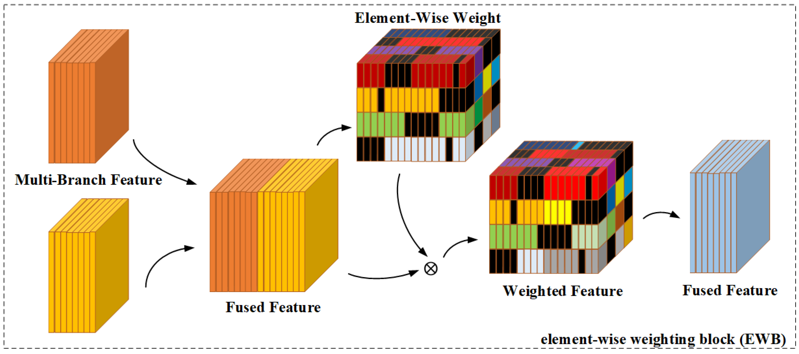
  • We propose an element-wise weighting block (EWB) module to perform high-fine-grained feature enhancement and suppression on feature cubes, addressing the limitations of simple channel attention and spatial attention mechanisms with low fine-grainedness.
  • We propose a chained deduced classification strategy (CDCS) to improve the overall accuracy of multi-temporal semantic segmentation tasks and ensure that the multi-temporal classification results are consistent with the real changes of ground objects.
  • To validate our proposed method, we make a large-scale multi-temporal Landsat dataset. Extensive experiments demonstrate that our method achieves state-of-the-art performance on Landsat images. The classification accuracy of our proposed method is much higher than other mainstream semantic segmentation networks.

2. Methodology

2.1. Multi-Temporal Network

UNet is a relatively simple and most commonly used encoder-decoder network. It is used as the baseline network in this work. UNet has low GPU memory overhead and fast running speed. We design a dual-branch encoder network to introduce the previous phase images and the corresponding ground-truth labels to assist the segmentation of the latter phase images. Each encoder branch extracts image features in different time phases. We take the ground-truth label of the previous phase as the known prior knowledge and input it into the network together with the image of the previous phase to assist the network learning. It makes the network focus more on the features of the changing area and reduces the difficulty of feature extraction. The network evolves from fully learning all feature information to focusing on learning the feature information of changing regions. When a certain position does not change, the category of the prior knowledge of the previous phase is directly brought into the classification result; when a certain position changes, the feature information of the ground object category before and after the change is learned by the network. At this time, feature learning is optimized from relatively dense learning to relatively sparse learning, significantly improving the network’s feature extraction ability. It can avoid the pseudo-change phenomenon caused by the difference in color distribution of images in different phases.
We named the input data of the two phases the reference phase data and the unknown phase data, respectively. Suppose the number of bands of the image is N. In that case, the reference phase data is formed by stacking the image and the corresponding label, so the number of input channels is N + 1 . We call this branch the reference branch. The unknown phase data is only image data, so the number of input channels is N. We call this branch the unknown branch. Both the reference branch and the unknown branch use the ResNet-50 [45] encoder for feature extraction. Since the number of channels of the input data of the two branches is different, the encoder weights are independent of each other and do not share weights. The features of each stage of the two encoders are fused by the EWB module. The fused features are transferred to the decoder for low- and high-level fusion. The decoder is a standard UNet decoder. We call this network architecture the dual temporal network (DTNet). The overall architecture of the DTNet is shown in Figure 3.
The DTNet can be denoted as follows:
f D T = f d e c ( f E W B ( f r e f ( x 1 N + 1 ) , f u n k ( x 2 N ) ) ) ,
where x 1 N + 1 represents the N + 1 band image and label input in the first phase, x 2 N represents the N-band image input in the second phase, f r e f represents the reference branch encoder, f u n k represents the unknown branch encoder, f E W B represents the EWB module, and f d e c represents the decoder.
The number of input channels of the two branches is N + 1 and N, respectively. Therefore, the network is an asymmetric two-branch network. In the training phase, the labels corresponding to the unknown phase data are used to calculate the loss value at the end of the network and guide the network backpropagation and gradient update. In the inference stage, we need to input the images and labels of the previous phase and the images of the latter phase to obtain the latter phase’s segmentation results.
Based on DTNet, we can introduce more previous phase images and the corresponding ground-truth labels to obtain richer temporal information and more stable ground object change information. Similar to the DTNet architecture, but in the encoder part, we add a new reference branch, which is used to extract features of the newly added reference phase data. The newly added reference branch is similar to the reference branch of DTNet. The image of this phase and the corresponding ground-truth label are stacked as input data. ResNet-50 is also used as the encoder to extract features. The number of input data channels of the two reference branches is N + 1 . To reduce the network’s number of parameters and the network’s training difficulty, we share the weights of the ResNet-50 encoders of the two reference branches. It means letting the same encoder extract the feature information from the first two reference phase data. After sharing the weights, the positions of the features extracted by the two reference branches in the feature cube can also be the same. So that the network can compare the differences between the two-phase features and learn the change feature information in the ground objects. During the backpropagation stage, when training the network, the two reference branches jointly update the weights of the same encoder. Since the number of input channels of the unknown branch is different from that of the reference branch, the unknown branch still uses an independent encoder and does not share weights. Like DTNet, the features of each stage of the three branches are fused by the EWB module. The decoder is a standard UNet decoder. We call this network architecture the triple temporal network (TTNet). The overall architecture of the TTNet is shown in Figure 4.
The TTNet can be denoted as follows:
f T T = f d e c ( f E W B ( f r e f ( x 1 N + 1 ) , f r e f ( x 2 N + 1 ) , f u n k ( x 3 N ) ) ) ,
where x 1 N + 1 and x 2 N + 1 represents the N + 1 band image and label input in the first and second phase, x 3 N represents the N-band image input in the third phase, f r e f represents the weight-sharing reference branch encoder, f u n k represents the independent unknown branch encoder, f E W B represents the EWB module, and f d e c represents the decoder.
The number of input channels of the three branches is N + 1 , N + 1 , and N, respectively. Two N + 1 branches are weight-sharing branches. Therefore, the network is an asymmetric weight-sharing three-branch network. In the training phase, the labels corresponding to the unknown phase data are used to calculate the loss value at the end of the network and guide the network backpropagation and gradient update. In the inference stage, we need to input the images and labels of the previous two phases and the images of the latter phase to obtain the latter phase’s segmentation results.
In theory, when there are more phase input data, more reference branches can be stacked to build a multi-temporal network (MTNet). The reference branch in the MTNet uses a weight-shared encoder, the unknown branch uses an independent encoder, and the multi-branch feature fusion uses the EWB module. MTNet is a plug-and-play network framework. In addition to using UNet, various mainstream semantic segmentation networks can be transformed into MTNet architectures. The more reference branches, the richer the temporal information of the ground objects and the more conducive to the network to exploit the feature information of the ground objects. The segmentation result of the last unknown phase can be classified more accurately.
The MTNet can be denoted as follows:
f M T = f d e c ( f E W B ( f r e f ( x 1 N + 1 ) , f r e f ( x 2 N + 1 ) , , f r e f ( x m 1 N + 1 ) , f u n k ( x m N ) ) ) ,
where x 1 N + 1 , x 2 N + 1 , …, and x m 1 N + 1 represents the N + 1 band image and label input in the first, second to the m 1 th phase, respectively, x m N represents the N-band image input in the mth phase, f r e f represents the weight-sharing reference branch encoder, f u n k represents the independent unknown branch encoder, f E W B represents the EWB module, and f d e c represents the decoder.

2.2. Element-Wise Weighting Block

We build a weight feature cube the same size as the original feature cube. Attention learning is performed for each spatial position and each channel, enhancing or suppressing the features of different channels at different spatial positions more flexibly. Compared with simple channel attention and spatial attention, our proposed element-wise weighting block (EWB) module can improve the fine-grainedness of attention weights. As shown in Figure 5, the color represents the enhanced feature, and the black represents the suppressed feature. According to the response of different categories of features at different spatial positions and channels, the network suppresses redundant useless information and enhances effective information, thereby improving the efficiency and accuracy of network learning. For multi-temporal branch feature fusion, the EWB module can exploit the effective information of different temporal features with high fine-grainedness and learn the change feature information by itself.
As shown in Figure 6, we first concatenate the features of multiple encoder branches to obtain the combined features. Then we use a 1 × 1 convolution operation to obtain initial feature weights and the rectified linear unit (ReLU) function to deactivate some features. Next, we use a 1 × 1 convolution operation again and then use the sigmoid function to transform the feature weights to obtain the final feature weights. The feature weights are weighted to the combined features to obtain weighted fusion features.
We express a convolution layer W n ( x ) as follows:
W n ( x ) = W n × n x + b ,
where ⊙ represents the convolution operator, W n × n represents the n × n convolutional kernel, b represents the vector of bias, and x represents the input data.
We denote the concatenation operation as follows:
x c o n c a t = x 1 x 2 ,
where ⊕ represents the concatenation operator, and x 1 and x 2 represents the features of the two branches.
The EWB module can be denoted as follows:
f E W B ( x ) = x c o n c a t ( f s i g m o i d ( W 2 1 ( f R e L U ( W 1 1 ( x c o n c a t ) ) ) ) ) ,
where ⊗ represents the dot multiply operator, f s i g m o i d represents the sigmoid function, f R e L U represents the ReLU function, W 1 1 and W 1 2 represents the first and second 1 × 1 convolution layer, respectively, and x c o n c a t represents the combined feature.

2.3. Chained Deduced Classification Strategy

Suppose we have 4 phase images, labeled I t 1 , I t 2 , I t 3 , and I t 4 , respectively. We also have the ground-truth labels for the two phases t 1 and t 2 , labeled L t 1 and L t 2 , respectively. The number of image phases of 4 and the number of label phases of 2 are only for ease of understanding. In practice, the phase number of both images and labels can be a larger value.
First, we use the images and ground-truth labels of the two phases t 1 and t 2 as samples and the DTNet in Section 2.1 for training. I t 1 , L t 1 , and I t 2 are the input data for the network, L t 2 is the label for supervised learning. We can obtain model M t 1 _ t 2 after training. We denote this process as follows:
f D T ( ( I t 1 + L t 1 ) , I t 2 ) L t 2 M t 1 _ t 2 ,
where f D T represents the DTNet, both sides of ‖ represent the network output and supervised learning labels, respectively, and ⇔ represents the training task, including forward and backward propagation.
Then, we use the trained model M t 1 _ t 2 to predict the classification result C t 3 of phase t 3 . The input data of the network is replaced by two phases t 1 and t 2 with two phases t 2 and t 3 . We denote this process as follows:
f D T ( ( I t 2 + L t 2 ) , I t 3 ) M t 1 _ t 2 C t 3 ,
where f D T represents the DTNet, both sides of ⊙ represent the data and model, respectively, and ⇒ represents the inference task, only including forward propagation.
Then we use the classification result C t 3 of phase t 3 as the pseudo label to train adaptively the model M t 2 _ t 3 for two phases t 2 and t 3 . We denote this process as follows:
f D T ( ( I t 2 + L t 2 ) , I t 3 ) C t 3 M t 2 _ t 3 ,
where f D T represents the DTNet, both sides of ‖ represent the network output and supervised learning labels, respectively, and ⇔ represents the training task, including forward and backward propagation.
Then we use the trained model M t 2 _ t 3 to predict the classification result C t 4 of phase t 4 . The input data of the network is replaced by two phases t 2 and t 3 with two phases t 3 and t 4 . We denote this process as follows:
f D T ( ( I t 3 + C t 3 ) , I t 4 ) M t 2 _ t 3 C t 4 ,
where f D T represents the DTNet, both sides of ⊙ represent the data and model, respectively, and ⇒ represents the inference task, only including forward propagation.
So far, we have completed the semantic segmentation of the two phases t 3 and t 4 . When we have more follow-up phase images, we can continue to deduce the new phase result according to the above rules.
In summary, we use the classification result C t [ n 1 ] of phase t [ n 1 ] as the pseudo label to train adaptively the model M t [ n 2 ] _ t [ n 1 ] for two phases t [ n 2 ] and t [ n 1 ] . We denote this process as follows:
f D T ( ( I t [ n 2 ] + C t [ n 2 ] ) , I t [ n 1 ] ) C t [ n 1 ] M t [ n 2 ] _ t [ n 1 ] ,
where f D T represents the DTNet, both sides of ‖ represent the network output and supervised learning labels, respectively, and ⇔ represents the training task, including forward and backward propagation.
Then we use the trained model M t [ n 2 ] _ t [ n 1 ] to predict the classification result C t [ n ] of phase t [ n ] . The input data of the network is replaced by two phases t [ n 2 ] and t [ n 1 ] with two phases t [ n 1 ] and t [ n ] . We denote this process as follows:
f D T ( ( I t [ n 1 ] + C t [ n 1 ] ) , I t [ n ] ) M t [ n 2 ] _ t [ n 1 ] C t [ n ] ,
where f D T represents the DTNet, both sides of ⊙ represent the data and model, respectively, and ⇒ represents the inference task, only including forward propagation.
We refer to this training/inference alternating classification strategy as the chained deduced classification strategy (CDCS). The schematic diagram of CDCS is shown in Figure 7. This idea can also be extended to TTNet and MTNet frameworks. This strategy requires that the classification results of the next phase be deduced sequentially in chronological order. Because the changing rules of some ground objects, such as residential areas, generally show an overall increasing trend, if the later phase is placed in the previous, it will cause the error phenomenon of “reduction of residential areas”.
Considering the real surface changes and the differences in the color distribution of multi-temporal images, the change feature information from t 1 to t 2 , t 3 or t 4 will be quite different. When the model M t 1 _ t 2 is directly applied to the t 3 or t 4 classification, the error will be larger than the CDCS. Therefore, the multi-temporal classification results using the CDCS will be more stable and consistent with the actual changes.

3. Experimental Results

3.1. Datasets

To test our proposed network architecture, we need multiple phases of images. Each phase of images is fully registered. Each phase of the image needs to have a corresponding classification label. The currently published remote sensing semantic segmentation datasets cannot meet the requirements of multi-phase image registration. Some remote sensing change detection datasets have multiple registered images, but each image is not labeled pixel by pixel. Only the change area is labeled in those change detection datasets. Therefore, it is indispensable to make our own Landsat dataset.
We choose parts of northern and southwestern China as the study areas. We downloaded Landsat images in 2000, 2005, 2010, 2015, and 2020, each containing 102 images. All downloaded images are at the L1TP level, and the surface reflectance data are obtained after FLAASH processing of ENVI software. We only used six bands of data, including blue, green, red, near-infrared, shortwave infrared 1, and shortwave infrared 2. We stitched images of the two study areas by year, cut out the redundant parts, and only kept the images in the study area. We finally cropped all images according to the standardized grid and obtained 20 tiles of images with 10 , 240 × 10 , 240 pixels each year. Region-I is the name defined for the study area in the northern China. It has 16 tiles covering an area of 1,440,000 km 2 and is located between 110 . 9 E 122 . 3 E and between 34 . 1 N 45 . 5 N . Region-II is the name defined for the study area in the southwest China. It has 4 tiles covering an area of 360,000 km 2 and is located between 102 . 4 E 108 . 1 E and between 28 . 4 N 34 . 1 N . As shown in Figure 8 and Figure 9, all images in 2000, 2005, and 2010 are pixel-level labeled, including 7 categories: woodland, grassland, wetland, waterbody, cultivated land, artificial surface, and bare land. As shown in Figure 10, the images in 2015 and 2020 are not labeled and are only used to visually evaluate the effect of the CDCS.
All samples were visually interpreted manually in ArcGIS software by a workgroup of more than ten people, within six months. Since some small ground objects are difficult to interpret visually, the workgroup used multi-temporal high-resolution images as a reference. In order to ensure high-quality labels, the entire workgroup has basic knowledge of landcover, and some controversial sample sites were confirmed through field surveys. All samples were randomly cross-checked three times, and disputed samples were uniformly determined. Although there is a certain possibility of error in manual labeling, we try our best to minimize it and make the label accuracy as close to 100% as possible.
The ground objects in the adjacent area have certain correlations and similarities, so the pixel value distribution on the image also has a certain correlation. Therefore, if all image slices are directly divided into the training sub-dataset and the test sub-dataset randomly, there is no way to de-correlate the two sub-datasets, resulting in an inaccurate evaluation of the model’s generalization ability. Therefore, we must keep the different sub-datasets in relatively independent geographic locations. As shown in Figure 11a, the inner 4 tiles (IDs 6, 7, 10, 11) of Region-I are used for the training and validation dataset. We name it Landsat dataset I (LSDS-I). The outer 12 tiles (IDs 1, 2, 3, 4, 5, 8, 9, 12, 13, 14, 15, 16) of Region-I are used for the test dataset. We name it Landsat dataset II (LSDS-II). To further validate the model’s cross-region generalization ability, the images in Region-II are chosen only for prediction and do not involve in the training stage. Region-II is far away from Region-I. As shown in Figure 11b, all 4 tiles (IDs 17, 18, 19, 20) of Region-II are used for the test dataset. We name it Landsat dataset III (LSDS-III).

3.2. Implement Details

3.2.1. Data Preprocessing

For LSDS-I, we cropped the big tiles of LSDS-I with a sliding window to generate 1600 small tiles with 512 × 512 pixels. We randomly divided the cropped tiles into training set and validation set in a ratio of 8:2. For LSDS-II and LSDS-III, these two datasets do not participate in training and validation. They are only used as test sets for generalization ability testing. Since the mainstream semantic segmentation network and our proposed MTNet are all fully convolutional neural networks, which can adapt to any image size. Therefore, LSDS-II and LSDS-III are not cropped. All bands in the data are used for training and prediction.
Three phases of samples are included in the three LSDS series datasets. The mainstream semantic segmentation network adapts to single-temporal input, our proposed DTNet adapts to dual-temporal input, and the TTNet adapts to triple-temporal input. To ensure that all three phases of samples can be trained in the single-temporal network and DTNet, we preprocessed the multi-phase samples. For the single-temporal network, we mix the three-phase samples together to generate pseudo-single-phase samples for training. For the DTNet, we mix the three-phase samples in pairs to generate pseudo-dual-temporal samples for training.
We normalize the training image data according to Equation (13) to conform to the network’s standard input format.
D = D m e a n s t d d e v ,
where D represents the normalized data, D represents the input data, m e a n represents the mean value of the corresponding channel in the training image data, and s t d d e v represents the standard deviation of the corresponding channel in the training image data.

3.2.2. Training Settings

PyTorch deep learning framework [46] is used to train the MTNet proposed in this paper. Some mainstream semantic segmentation models are also implemented by the PyTorch framework. We use four NVIDIA RTX 3090 GPUs with 24 GB memory each GPU for training. The data augmentation operations include random horizontal flip, random vertical flip, and random rotation. We choose 32 as the batch size and AdamW [47] as the optimizer. The initial learning rate LR is set to 1 × 10 5 . First, we use a warm-up strategy to adjust LR. According to Equation (14), the LR rises to 1 × 10 3 after 10 epochs. Then, we use reduce-LR-on-plateau strategy to adjust LR. According to Equation (16), the LR is multiplied by a factor of 0.3 if the validation accuracy does not increase in 20 epochs. The training process will be stopped if the LR is lower than 1 × 10 7 .
l r = l r 0 · ( l r * l r 0 ) t n ,
where l r represents the current LR, l r 0 represents the initial LR, l r * represents the LR after the warm-up stage, t represents the current iteration number, and n represents the total iteration number in the warm-up stage. n is defined as follows:
n = e · k ,
where e represents the total epoch number, and k represents the iteration number per epoch.
l r = α · l r ,
where l r represents the current LR, l r represents the last LR, and α represents the adjustment factor in the reduce-LR-on-plateau stage.
To speed up network convergence and improve learning ability, we use cross-entropy loss to calculate pixel-level loss and Lovasz-softmax loss to calculate region-level loss simultaneously. To avoid the effects of differences in hardware and hyperparameters, we configure each model training with the same hardware and hyperparameters. There will be random errors in the training stage, resulting in slight fluctuations in the accuracy of each training. To make the accuracy more objective, we randomly trained each model 10 times. We compute the average accuracy of each model as the metric of the final accuracy comparison.

3.2.3. Evaluation Metrics

Overall accuracy (OA) is the proportion of correctly classified pixels, which can be defined as follows:
O A = { y = y ^ } { y = y ^ } { y y ^ } ,
where y represents the ground truth of samples, and y ^ represents the predicted results.
Each single-class accuracy uses the F 1 score as the evaluation metric. True positive (TP) means that the sample is true and the prediction result is also true. False positive (FP) means that the sample is false and the prediction result is true. False negative (FN) means that the sample is true and the prediction result is false. The p r e c i s i o n and r e c a l l can be calculated by TP, FP, and FN as follows:
p r e c i s i o n = T P T P + F P ,
r e c a l l = T P T P + F N
Therefore, the F 1 score is defined as follows:
F 1 = 2 · p r e c i s i o n · r e c a l l p r e c i s i o n + r e c a l l
Since OA is not sensitive enough to the category with a small proportion [48], we additionally use mean F 1 score ( mF 1 ) as the second metric for the overall evaluation. The mF 1 is defined as the mean of the F 1 scores for every category, shown as follows:
mF 1 = 1 N i = 1 N F 1 i ,
where F 1 i represents the F 1 score of the ith category, and N represents the number of categories.

3.3. Experiments on the Landsat Dataset I

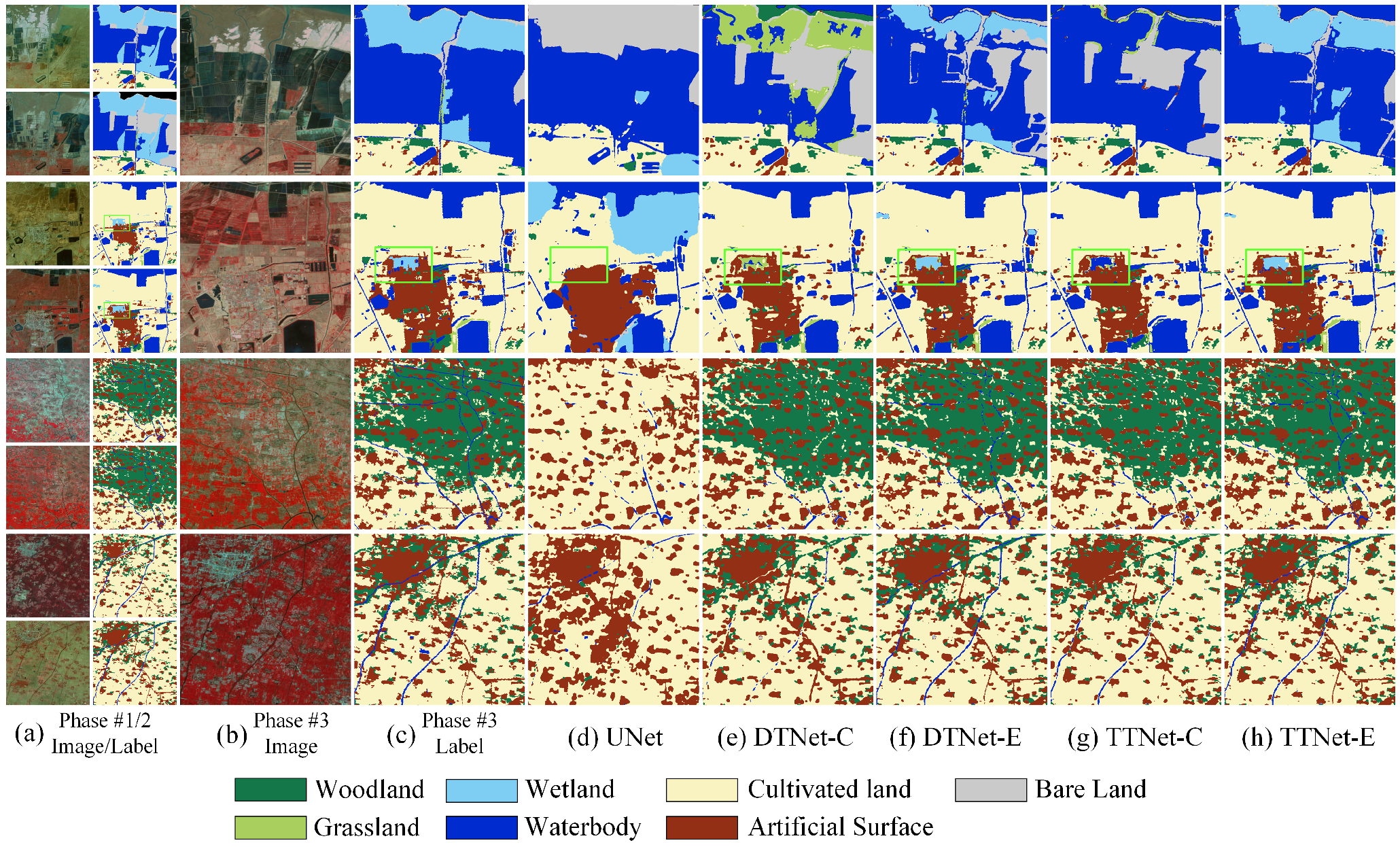
3.3.1. Ablation Study

Based on the baseline UNet, we incrementally build DTNet and TTNet in turn and introduce the EWB module to evaluate the effect of each module and structure on improving the classification accuracy. Table 1 shows the ablation comparison accuracy of the MTNet on the validation set of LSDS-I. The OA of UNet is 81.1%. We add a reference branch and use the Concat method for dual branch fusion to build the network DTNet-C. Due to the prior information and constraints provided by the previous phase data, the accuracy of each category has been increased. The accuracy of bare land has been greatly increased. The OA of DTNet-C has reached 89.4%. We further add the previous reference branch and still use the Concat method to achieve triple branch fusion to build the network TTNet-C. Since we have obtained richer temporal information and more change feature information in ground objects, the accuracy of all classes has been further increased. The OA of TTNet-C has reached 90.6%. To verify the effect of the EWB module, we replace the Concat modules of DTNet-C and TTNet-C with the EWB module to build DTNet-E and TTNet-E, respectively. Since the EWB module allows the network to select effective features more efficiently from multi-branch features and reduce the interference of redundant and useless features, the accuracy of all classes has been greatly increased compared to the Concat fusion method. On the Landsat image, two groups of easily confused ground objects, wetland/waterbody and grassland/bare land, are better distinguished with the help of the EWB module. Therefore, the accuracy of those confused categories is improved obviously. The accuracies of DTNet-E and TTNet-E reach 91.3% and 93.2%, respectively. Compared with the baseline UNet, the accuracy of the best MTNet member TTNet-E proposed in this paper is improved by 12.1%.
The visualization results of our proposed MTNet family networks and the baseline UNet on LSDS-I are shown in Figure 12. In the first row, UNet cannot extract the wetlands in the red rectangle. Although DTNet-C has added a reference branch, there is no EWB module to filter and optimize the multi-branch effective features. Therefore, the wetlands are misclassified. Also, the grassland is wrongly classified as woodland in the lower right corner. TTNet-C introduces richer temporal information, but without the help of the EWB module, it misclassifies wetlands as waterbodies. DTNet-E can correctly extract wetlands. However, due to the short phase, the network only obtains information about previously cultivated land from the previous phase. Therefore, the waterbody is misclassified as cultivated land. Under the optimization of rich temporal information and the EWB module, TTNet-E has learned the change feature information in ground objects. Therefore, the waterbodies and wetlands in this area are correctly classified. In the second row, UNet mistakenly classifies the wetland in the yellow rectangle as woodland. The artificial surface is also roughly classified, and the woodland is incorrectly classified into cultivated land. After DTNet-C and TTNet-C introduced the image and label information of the previous phase, the misclassification problem of large areas of woodland was solved. However, the wetland in the yellow rectangle was still wrongly classified as grassland. The boundary detail of the artificial surface is improved, but the river has disconnection problems. After DTNet-E and TTNet-E introduced the EWB module, the multi-branch features were filtered and optimized. The wetlands in the yellow rectangle were correctly classified, and the river connectivity was better. The boundaries between ground objects were more accurate. In the third and fourth rows, the details of small objects have been greatly improved after adding the previous phase label information. From the results, the MTNet and EWB module proposed in this paper are effective, especially for small targets and boundary details optimization.

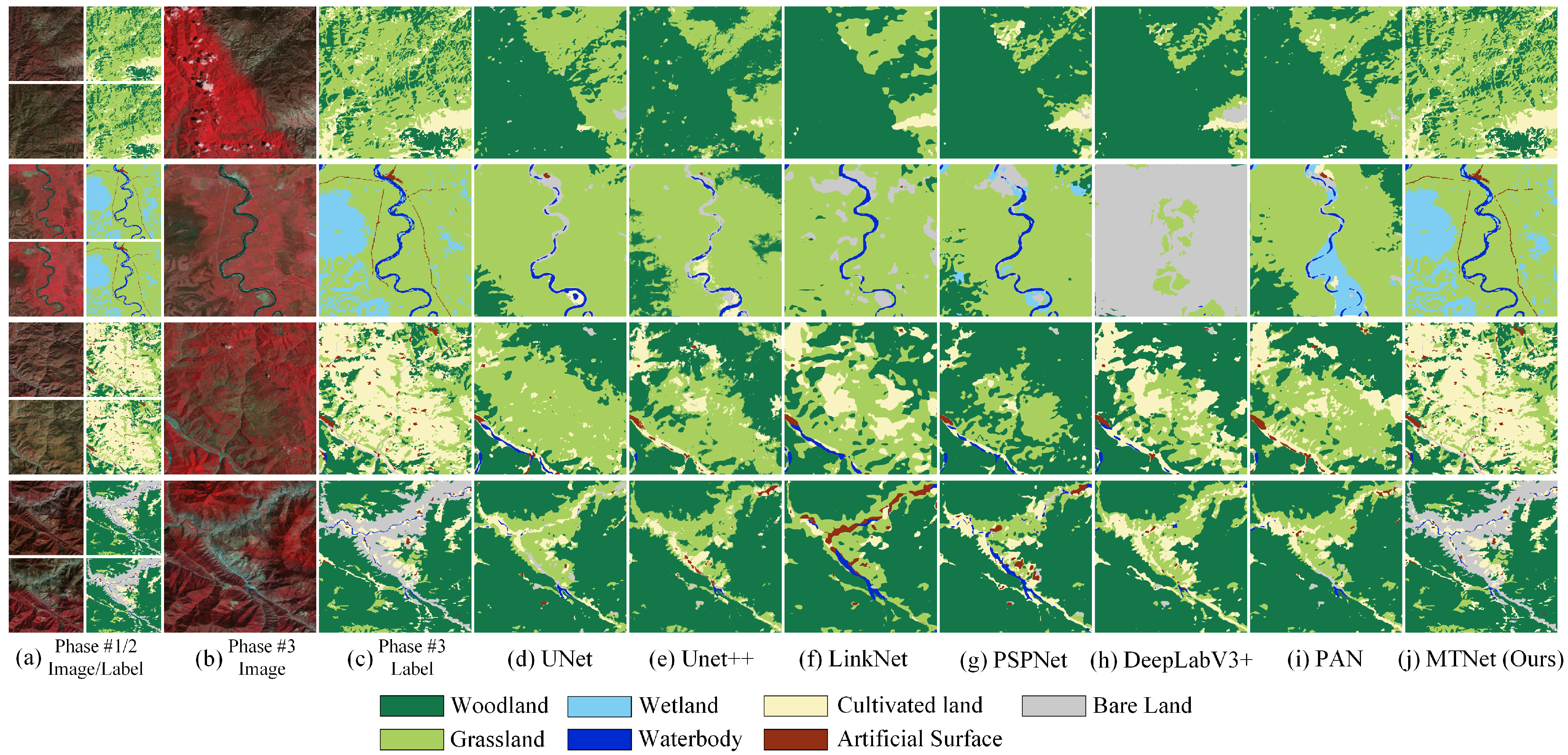
3.3.2. Comparing Methods

We trained some mainstream semantic segmentation networks and our best-performing MTNet member TTNet-E on LSDS-I. Table 2 shows that the OA of mainstream networks is around 79% to 81%, but TTNet-E can reach 93.2%. All categories’ accuracy is much higher than mainstream networks, which perform poorly on bare land. However, TTNet-E improves the accuracy of bare land to 81.1%, and the improvement of other categories is about 13.6% to 33.1% compared to UNet.
The mainstream semantic segmentation networks we trained in this work are listed as follows:
(1)
UNet [33]: UNet uses an encoder to extract each stage’s features as spatial feature information. The decoder gradually restores the original size of the pooled features and fuses them with the corresponding spatial feature information of the encoder.
(2)
UNet++ [49]: UNet++ adds more node modules in each stage of UNet’s decoder, making feature processing more intensive.
(3)
LinkNet [50]: LinkNet simplifies the network structure and accelerates the speed of network training and prediction while ensuring accuracy, thereby implementing real-time segmentation tasks.
(4)
PSPNet [31]: PSPNet replaces the ordinary convolution in the encoder with dilated convolution, which can maintain the resolution of the features. It uses the SPP module to extract features of different scales and perform multi-scale feature fusion.
(5)
DeepLabV3+ [51]: DeepLabV3+ is a hybrid-style network that integrates backbone style and encoder-decoder style. It replaces the ordinary convolution operation in the encoder with atrous convolution, which preserves the resolution of features. It uses the ASPP module to extract features of different scales and perform multi-scale feature fusion.
(6)
PAN [52]: PAN extracts multi-scale features by the feature pyramid attention (FPA) module, and progressively fuse the multi-scale features by the global attention upsample (GAU) module.
(7)
MTNet: Our MTNet is a network by adding the reference data of the previous two phases and the EWB module based on UNet, namely TTNet-E. Since TTNet-E is the best performer on LSDS-I in the MTNet member networks, we denote the TTNet-E in Section 3.3.1 as MTNet here.
Figure 13 shows the visualized results of MTNet and mainstream networks on the LSDS-I. In the first row, the mainstream networks cannot correctly extract the bare land, and the grass in the upper left corner was incorrectly classified as woodland. However, MTNet relies on multi-temporal information constraints and the EWB module optimization to correctly classify bare land and grassland, and the boundaries of ground objects are excellent. In the second row, the location distribution of woodland, grassland, and wetland is very complicated, and there is a certain degree of confusion. The mainstream networks have poor classification results in this area. The artificial surface also cannot extract correctly in the lower left corner. However, MTNet can effectively classify complex and interlaced ground objects after the feature optimization of the EWB module. The classification result is very close to the label, and the accuracy is very high. In the third and fourth rows, there are a lot of misclassifications in other mainstream models. MTNet relies on the pre-phase label and the change information constraints to improve classification accuracy significantly. Therefore, the MTNet proposed in this paper far exceeds the current mainstream networks and reaches the state-of-the-art level.

3.4. Experiments on the Landsat Dataset II

3.4.1. Ablation Study

We performed prediction and accuracy evaluation on LSDS-II to test our proposed model’s generalization ability on Landsat images. Table 3 shows that all networks’ accuracy decreases slightly relative to LSDS-I. LSDS-I is used for accuracy validation in the training stage. The best model weights are selected according to the accuracy of the LSDS-I validation set. Whereas LSDS-II is only used for prediction, the accuracy of the same model is usually lower on LSDS-II than on LSDS-I. The accuracy of our proposed TTNet-E still has a significant improvement on LSDS-II, which can achieve 91.3% OA. It indicates that our MTNet has good generalization ability.
The visualization results of our proposed MTNet family networks and the baseline UNet on LSDS-II are shown in Figure 14. In the first row, waterbodies and wetlands are the main ground objects. UNet, without the help of pre-phase information, mistakenly classified wetlands into bare land. On Landsat images, wetlands and grasslands are easily confused. Therefore, DTNet-C did not use the EWB module to filter and optimize features, so the wetlands were mistakenly classified as grasslands. Wetlands and waterbodies are also prone to confusion. Therefore, TTNet-C incorrectly classified wetlands into waterbodies without the EWB module. After introducing the EWB module, DTNet-E can correctly extract most of the wetlands. However, the two-branch network has limited change information on the ground objects. Under the influence of the bare land in the previous phase, many waterbodies are wrongly classified as bare land. TTNet-E has further optimized the classification results through richer change feature information in ground objects and feature selection and optimization of the EWB module. In the second row, the artificial surface classified by UNet is relatively rough. A large number of cultivated land are also wrongly classified as wetlands. Without the EWB module, both DTNet-C and TTNet-C misclassify a small wetland in the middle as grassland or waterbody. TTNet-E solves the problem of change information learning and multi-branch effective feature selection and optimization. Therefore, the classification result has been significantly optimized. In the third and fourth rows, it can be clearly seen that after adding the pre-phase label information, the long and narrow objects can be correctly extracted, and the details have been greatly improved. Therefore, the MTNet family and EWB module proposed in this paper have excellent generalization ability on multi-temporal Landsat images.

3.4.2. Comparing Methods

We performed prediction and accuracy evaluation on LSDS-II to test our proposed model’s generalization ability on Landsat images and compare it with the mainstream networks. TTNet-E is chosen as the representative of MTNet. As shown in Table 4, although the accuracies of all models have a slight drop on LSDS-II, TTNet-E still outperforms other mainstream networks with 91.3% OA. Compared with the best performing UNet and PAN in mainstream networks, the accuracy is improved by 13.1%. The mainstream networks used for comparison are the same as Section 3.3.2. Our TTNet-E continues to be denoted as MTNet here.
Figure 15 shows the visualized results of MTNet and mainstream networks on the LSDS-II. In the first row, MTNet can correctly extract the woodland below, and the details of the artificial surface are more accurate. However, other networks cannot effectively distinguish the woodland from the cultivated land, and parts of the artificial surface have been missed. In the second row, MTNet, with the help of the pre-phase information, the outline of the woodland is very accurate, and the artificial surface can also be completely classified. However, the woodland boundaries extracted by other networks are very inaccurate, and there are a lot of omissions on the artificial surface. In the third and fourth rows, other mainstream networks have the phenomenon that small objects are missed, and large areas are misclassified. With the help of the pre-phase information, the MTNet is more focused on the feature information extraction of the changing area, preventing the unchangeable area from misclassifying and significantly improving the classification accuracy. Therefore, the MTNet proposed in this paper has advanced performance and good generalization ability.

3.5. Experiments on the Landsat Dataset III

We performed prediction and accuracy evaluation on LSDS-III to further test our proposed model’s generalization ability on multi-temporal Landsat images. As shown in Table 5, since Region-II is far away from Region-I, the accuracy of all models dropped in a certain. Since DCNN is trained for the existing scene in the sample, the accuracy will inevitably drop when facing a scene that has not been faced before. At this time, the accuracy retention ability can indicate the model’s generalization ability. Our proposed MTNet mainly focuses on the changed information. When the network thinks that a certain region has not changed, it will retain the label of the previous phase as the classification result. Hence, the stability of the classification result for MTNet is very high. On LSDS-III, the accuracy drop of MTNet is very small. It is obvious that MTNet still has a strong generalization ability. The MTNet can still achieve 90.1% OA on LSDS-III, far exceeding other mainstream networks. Since other mainstream networks need to learn complex features and have poor adaptability to unfamiliar scenes, the generalization ability is severely reduced. However, the MTNet mainly focuses on changing feature information and has strong adaptability in the face of unfamiliar scenes, so it can still keep the good generalization ability. Figure 16 shows the visualized results of MTNet and mainstream networks on the LSDS-III. Obviously, other mainstream networks have many misclassifications due to their poor generalization ability, while MTNet can still keep the high classification accuracy.

3.6. Experiments for Chained Deduced Classification Strategy

3.6.1. Experimental Settings

To test the robustness and generalization ability of the CDCS, we reserve all the samples in 2010, do not use them for training, and only for inference and accuracy evaluation. Therefore, there are only two phases of samples in 2000 and 2005 used for training. We choose the DTNet for the CDCS experiment. In addition, there are two phases of unlabeled images in 2015 and 2020, which are also used for prediction and only evaluation visually. To compare with the mainstream single-temporal networks, we mixed the samples in 2000 and 2005 for training and performed classification on three phases of images in 2010, 2015, and 2020. We used the classification results in 2010 to calculate the quantification accuracy and the classification results in 2015 and 2020 to evaluate accuracy visually.
All data preprocessing operations and network training settings are the same as in Section 3.2. For the CDCS of the DTNet, we first stack the samples in 2000 and 2005 as the dual-temporal samples to train the model M 00 _ 05 . Then, we stack the samples in 2005 and images in 2010 and use the model M 00 _ 05 to predict the classification results in 2010. To make the model weight distribution closer to the image features in 2005 and 2010, we regard the classification results in 2010 as pseudo-labels and train the model M 05 _ 10 for the two phases of 2005 and 2010. Then, we stack the images in 2010, the corresponding classification results in 2010, and images in 2015, and use the model M 05 _ 10 to predict the classification results in 2015. Next, according to the rules mentioned above, we continue to regard the classification results in 2015 as pseudo-labels and train the model M 10 _ 15 for the two phases of 2010 and 2015. Finally, we stack the images in 2015, the corresponding classification results in 2015, and images in 2020, and use the model M 10 _ 15 to predict the classification results in 2020. For the DTNet without CDCS, we first stack the samples in 2000 and 2005 as the dual-temporal samples to train the model M 00 _ 05 . Then, we stack the samples in 2000 and images in 2010 and use the model M 00 _ 05 to predict the classification results in 2010. Then we repeat the prediction tasks in 2015 and 2020, both using 2000 samples as constraints and M 00 _ 05 as the model. For the mainstream single-temporal networks, firstly, the mixed pseudo-single-temporal samples in 2000 and 2005 are input for training, and then the images of 2010, 2015, and 2020 are classified by pixel level.

3.6.2. Ablation Study

Table 6 shows the quantitative accuracy comparison of the baseline UNet, MTNet without CDCS, and MTNet with CDCS. For convenience, our DTNet-E is noted as MTNet here. LSDS-I and LSDS-II located in Region-I were evaluated for accuracy together, and LSDS-III located in Region-II was independently evaluated for accuracy to compare the geospatial generalization ability. All models were optimized with the data in 2005 as the training target. The data in 2010 were not used for training, which was used to compare the multi-temporal generalization ability. Since the 2005 results of MTNet without CDCS and MTNet with CDCS were predicted by the same model, and CDCS began to work in the 2010 results, the 2010 results and labels were used for accuracy evaluation. It can be seen that CDCS has improved the network performance. Although it is less than the improvement brought by the multi-temporal reference branch, it still has an improvement effect. It is because, in CDCS, the model undergoes deduced training and gradually adapts to the next phase image’s color distribution and feature pattern. The classification results in the next phase have a more stable performance. Without the assistance of CDCS, the model is prone to unstable classification results due to differences in image color distribution.
The data in 2015 and 2020 have only images, and no corresponding ground-truth labels, so qualitative analysis and evaluation are mainly performed by visual inspection. To verify and compare the effect of CDCS in MTNet, we put the classification results in 2005, 2010, 2015, and 2020 together to obtain a multi-temporal classification result sequence. Figure 17 shows the multi-temporal classification results of MTNet without CDCS and MTNet with CDCS in Region-I. In the first group, without the help of CDCS, a large number of artificial surface false detections appeared in the 2015 results. After adding CDCS, the consistency of multi-temporal classification results was significantly improved. In the second group, without the support of CDCS, the 2015 and 2020 results showed an obvious false explosion of growth on the artificial surface. With the constraints of CDCS added, false classification results are suppressed. The growth trend of the artificial surface is more in line with the actual situation. In the third group, without the assistance of CDCS, the 2020 classification results showed an unreasonable explosion of artificial surfaces. Under the action of CDCS, the problem of false detection has been solved, and the growing trend of the artificial surface is more in line with the actual situation.
Figure 18 shows the multi-temporal classification results of MTNet without CDCS and MTNet with CDCS in Region-II. In the first group, in the absence of CDCS, the artificial surface was reduced anomalously in the 2020 results. With the assistance of CDCS, the artificial surface shows a gradual and slight growth trend, which is more in line with the actual situation. In the second group, when there is no CDCS, the classification results show an abnormal phenomenon of more and fewer waterbodies. Under the constraint of CDCS, abnormal waterbody results are suppressed, and the consistency of classification results is improved significantly. In the third group, without CDCS, the 2015 results showed a large amount of grassland, while the other years were woodland. With the help of CDCS, the falsely detected grasslands were suppressed, and the multi-temporal classification results had excellent consistency.
It can be seen that, although the overall consistency is good, when the color difference of the image is apparent, the artificial surface, waterbody, and grassland are prone to false detection, resulting in a wrong trend of change. The CDCS can gradually adapt to the color distribution and feature pattern of the next phase image, thereby significantly improving the consistency of multi-temporal results.

3.6.3. Comparing Methods

Table 7 shows the quantitative accuracy comparison between the mainstream single-temporal networks and our proposed MTNet with the CDCS. For convenience, our DTNet-E is noted as MTNet here. LSDS-I and LSDS-II located in Region-I were evaluated for accuracy together, and LSDS-III located in Region-II was independently evaluated for accuracy to compare the geospatial generalization ability. All models were optimized with the data in 2005 as the training target. The data in 2010 were not used for training, which was used to compare the multi-temporal generalization ability. It can be seen that the overall performance of the MTNet is greatly higher than that of single-temporal networks. From 2005 to 2010 in Region-I, the accuracy of each category of the single-temporal networks decreased to varying degrees. The wetland category decreased very seriously, even lower than 10% OA. The single-temporal networks completely lose the generalization ability for the multi-temporal classification task of wetland categories. However, the accuracy of each category of the MTNet is kept, with only a slight decline. Considering that the samples in 2010 were participating in the training stage, this decline is normal. The single-temporal network cannot solve the wetland generalization problem. However, MTNet can keep 78.2% OA for the wetland category. It shows that the MTNet fully uses the advantages of multi-temporal data in multi-temporal tasks and has outstanding generalization ability. For LSDS-III, which does not participate in the training stage and has a very low geographic correlation, the accuracy of each category of the single-temporal networks also decreases to varying degrees. In addition to the severe decline in the accuracy of wetlands, the accuracy of grasslands, waterbodies, and artificial surfaces has also dropped significantly. That is to say, the generalization ability of single-temporal networks in both geographic space and temporal changes is fragile. However, in unfamiliar geographic scenes, MTNet can enhance the learning of changing information with the help of multi-temporal information and reduce the burden of unchanging information in the feature extraction stage. It has a powerful generalization ability regarding geographic space and temporal changes.
The data in 2015 and 2020 have only images, and no corresponding ground-truth labels, so qualitative analysis and evaluation are mainly performed by visual inspection. Table 7 shows that the overall performance of the single-temporal networks is relatively similar. Therefore, we choose UNet++ as the representative of the single-temporal network and compare it with the MTNet with the CDCS. To compare the effect of the MTNet with the CDCS, we put the classification results in 2005, 2010, 2015, and 2020 together to obtain a multi-temporal classification result sequence. Figure 19 shows the multi-temporal classification results of UNet++ and MTNet in Region-I. In the first group, the classification results of UNet++ will miss a lot of small ground objects and details, such as woodlands, small villages, and roads. Residential areas increased significantly in 2015 but declined obviously in 2020. The changes in the residential area are completely inconsistent with the real scene. MTNet can effectively extract small ground objects and keep good details. The residential area is gradually increasing, in line with the real natural scene. In the second group, the results of UNet++ showed that the grassland and cultivated land changed repeatedly, but the cultivated land should not change greatly in the actual scene. In addition, the details of the classification results are poor. MTNet can keep the distribution of grassland and cultivated land stable with few changes. Only the artificial surface has a slight increase. It shows that MTNet has good stability and consistency. In the third group, the results of UNet++ are not stable enough. Although there is no major change in the ground objects from the image, the results are chaotic changes among woodland, grassland, waterbody, bare land, artificial surface, and cultivated land, which are completely inconsistent with reality. MTNet can keep the stability of the classification results with only a few changes, which is consistent with the real situation. It can be seen that UNet++ cannot establish multi-temporal correlation and the classification results are unstable. Obvious errors that do not conform to the actual situation always occur. The results of MTNet are consistent with the real changes in ground objects. It has good stability and consistency. It also has a strong ability to keep details.
Figure 20 shows the multi-temporal classification results of UNet++ and MTNet in Region-II. In the first group, UNet++ was unable to separate the relatively finely fragmented grassland in the upper right corner from the woodland. The wetland changed too much, and the waterbody was missed by UNet++. The surrounding woodland was misclassified. MTNet can keep the outline of the wetland, and the waterbody in the wetland is increased, which is consistent with the image. In the second group, the woodland, grassland, and cultivated land in the UNet++ results have changed too much. But from the image, the change in this area is very small. MTNet can keep the stability and consistency of classification results. In the third group, UNet++ missed a lot of small ground objects. In 2015, there were many false detections of woodland, and in 2020, there were many unreasonable increases in residential areas. MTNet can effectively extract small ground objects. The residential area gradually increases, which is in line with the law of natural development. The results of UNet++ and MTNet on Region-II are similar to that on Region-I. Obviously, the MTNet has better time deduction logic than the single-temporal network.
To sum up, MTNet with the CDCS has excellent stability, robustness, and powerful spatial-temporal generalization ability when facing multi-temporal classification tasks. For multi-temporal classification, single-temporal networks cannot establish the temporal correlation of ground objects, and images of different phases will be regarded as a new region to a certain extent. Due to differences in imaging conditions and image preprocessing, the color distribution of similar objects in different phases is different, resulting in inconsistent classification results, serious misclassification, abnormal changes in ground objects, and inconsistency with natural laws. The MTNet uses the help of the pre-phase samples to establish the change feature information of the ground objects and reduce the interference caused by the pseudo color changes of the images. In addition, MTNet makes the model continuously adapt to the characteristics of the following phases by alternating training/prediction, keeping the stability and consistency of multi-temporal classification, and the changes of ground objects conform to natural laws.

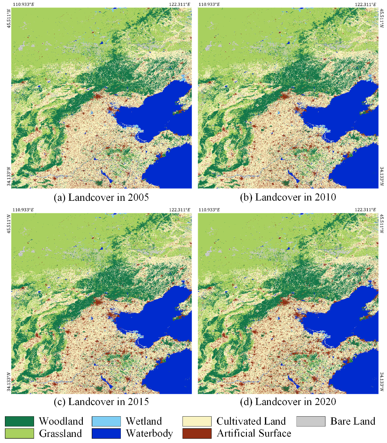
3.7. Large-Scale Multi-Temporal Landcover Mapping

We finally adopted the DTNet-E and the CDCS as the representative of the MTNet to classify Landsat images in 2005, 2010, 2015, and 2020 in the two study areas. We stitched all the classification results by year. Figure 21 and Figure 22 show the large-scale multi-temporal classification results of Region-I and Region-II, respectively. Intuitively, the classification results have been greatly improved with the help of multi-temporal label prior knowledge and change feature information. Our proposed MTNet has strong generalization ability on multi-temporal Landsat images and good robustness, stability, and consistency. The change of landcover is in line with the real situation of 15 years, which has a high research and application value.

4. Discussion

4.1. Trade-Off Problem

The MTNet and CDCS proposed in this paper can effectively solve the consistency problem of multi-temporal classification, but there are some trade-off problems in accuracy and efficiency.
The trade-off problem of sample labeling and multi-temporal consistency. MTNet has high requirements for samples, requiring at least two samples that have been strictly registered, and the preparatory work is relatively large. However, after the samples are prepared, the multi-temporal landcover classification can be completed very quickly. It has excellent consistency and can be used for quantitative analysis of landcover changes. The traditional mainstream single-temporal network has low requirements for sample labeling and small preparatory work. But it cannot guarantee multi-temporal consistency, and the classification results have poor details, which cannot ensure the accuracy requirements of quantitative analysis. Therefore, we can choose the traditional single-temporal network or the MTNet proposed in this paper according to the actual application requirements.
The trade-off problem of parameter quantity and multi-temporal consistency. When using CDCS to deduce the multi-temporal landcover classification, it is necessary to train a model for each phase, so the number of parameters of the model inevitably increases linearly. The linear dynamic grown amount of parameters is directly related to the number of phases, which will not cause explosive uncontrollability. The multi-temporal consistency can be significantly improved. Therefore, according to the actual computing resources, we can choose whether to use CDCS in MTNet.
The trade-off problem of running time and multi-temporal consistency. When using CDCS to deduce the multi-temporal landcover classification, in addition to the linear increase in the number of parameters, the running time also increases linearly. CDCS will improve the adaptation of the model to the image color distribution through time-phased training, thereby further improving the consistency of the results of multi-temporal landcover classification. Therefore, it is possible to choose whether to use CDCS in MTNet according to the limitation of actual computing time.
Table 8 shows the effects of CDCS on the number of parameters, training time, and inference time. It can be seen that since MTNet has one more encoder branch, the amount of network parameters is directly doubled compared to UNet. Without the use of CDCS, the running time difference between UNet and MTNet is not much different. Since MTNet is twice the size of UNet, it is normal for a slight drop in running speed. After using CDCS, the number of network parameters and the running time increases linearly.
In summary, the MTNet and CDCS proposed in this paper must be selected according to the application requirements. Traditional single-temporal networks are used when we cannot obtain multi-temporal registered samples. Our proposed MTNet is used when we need good consistency. When storage resources are limited, and large models cannot be deployed, MTNet without CDCS can be used. MTNet without CDCS is used when there is a strict limit on the running speed and cannot be trained multiple times. When only pursuing high precision and excellent multi-temporal consistency, and there is no computational resource limitation at all, we can use NTNet with CDCS.

4.2. Implications and Limitations

The MTNet proposed in this paper solves two critical problems of classical semantic segmentation networks in multi-temporal landcover classification. The first problem is that the classical networks only perform feature extraction and classification on single-temporal images and do not establish the association between multi-temporal images and labels. The second problem is that when the classical networks perform multi-temporal classification, the classification results are not stable enough, the consistency is poor, and the changes in ground objects do not match the real situation.
Based on the classic semantic segmentation network, this paper introduces the images and labels of the previous phase, and extends the network to a multi-branch network. Since the labels of previous phases are input to the network as prior knowledge, the network evolves from classical dense full-semantic learning to sparsely focused learning. It dramatically reduces the difficulty of the network’s feature extraction and network training. With the help of the pre-phase label information, it will not be affected by the difference in the color distribution of the image. Only when the change is obvious, the network regards the position as a change to avoid the interference of pseudo-changes. In a classic network, small objects tend to be swallowed by larger objects around them. Thanks to the reduced burden of sparse key learning on network feature expression, the multi-temporal network can pay attention to more detailed features, and small objects that are difficult to classify can also be accurately extracted. For the more difficult categories that are easy to confuse, the pre-phase label can play a very key reference role. Therefore, the accuracy of each category of the multi-temporal network is very high, and the anti-interference ability is very strong, so there is no need to worry about the long-tail effect that is most often encountered in semantic segmentation. Since MTNet focuses on whether the two images have changed, it still has a very good generalization ability when the image to be classified is quite different from the sample. However, the classical semantic segmentation network often suffers from serious degradation in accuracy due to sample mismatch and cannot be used.
We have made minor modifications to the common attention mechanism, making the weight cube in the attention module more fine-grained, enabling finer filtering and optimization of features. Due to the characteristics of sparsely focused learning in MTNet, the feature cube will have many useless and redundant features. The EWB module can fine-tune the optimized features, which can be used together to improve the classification accuracy further. However, the improvement of the EWB module is small, and the main contribution is provided by MTNet. MTNet can actually be regarded as a plug-and-play framework, and any classical semantic segmentation network can be upgraded to MTNet by adding reference branches. It can simultaneously take advantage of the high-performance feature extraction capability of state-of-the-art semantic segmentation networks and the sparsely focused learning of MTNet.
In the multi-temporal classification task, when the time span of the images to be classified is large, the training/prediction is alternated phase by phase so that the model can continuously adapt to the characteristics of subsequent phase images. Classical semantic segmentation networks tend to use all available samples, in conjunction with a large number of data augmentation strategies, to try to simulate the color distribution of images to be classified. However, it is often encountered that the difference in color processing is too large, which leads to the abnormal phenomenon that the variation range of the ground objects in the multi-temporal classification results is outrageous, or even more and more suddenly less. In multi-temporal classification tasks, many errors occur in single-temporal networks. The advantage of MTNet is that it focuses on learning the features of changing regions. The advantage of CDCS is that it controls the magnitude of change and continuously adapts to the changing features gradually. Therefore, MTNet with CDCS can ensure that in multi-temporal classification, the classification results can be deduced phase by phase, the classification accuracy can be kept at a high level, and the change rule is completely consistent with the real situation. Since the deep learning network relies on big data-driven training and has certain fault tolerance, the error in CDCS is within an acceptable range.
All in all, compared with mainstream single-temporal semantic segmentation networks, the method proposed in this paper works by introducing additional reference constraint information. It has solved the consistency problem encountered in multi-temporal semantic segmentation from another perspective and greatly improved the classification accuracy and the stability of multi-temporal classification. This method is helpful for studying the changes in landcover and can be applied to scenarios such as urban expansion, cultivated land changes, geological disaster monitoring, ecological and environmental protection, wetland monitoring, woodland protection, etc., and has significant application value.
However, this method also has certain limitations, requiring strict registration of multi-temporal images. Additional one-phase images and labels are required as reference input in both the training and prediction stages. Therefore, if there is only one phase sample, the method proposed in this paper will not be applicable. In future research, we will explore using samples in non-corresponding positions as reference constraint information to reduce the dependence and limitations on multi-temporal registered samples. Since few-shot learning, self-supervised learning, and active learning have gradually become more popular, we will try to build no-label or less-label models in our future research work.

5. Conclusions

In this paper, we proposed a multi-temporal network. Based on the single-temporal semantic segmentation network, we added one or more reference phases of samples as prior constraint knowledge, which solves the problem of pseudo changes and misclassification caused by the difference in color distribution of images in different phases. We proposed an element-wise weighting block module, which improves the attention weight’s fine-grainedness and can improve feature cubes’ filtering and optimization effect. We proposed a chained deduced classification strategy, which improves the stability and consistency of multi-temporal landcover classification and ensures that the multi-temporal classification results are consistent with the real changes of ground objects. In large-scale multi-temporal Landsat landcover classification, our method surpasses most mainstream networks, achieves state-of-the-art performance, and has strong robustness and generalization ability. In future research, we will generalize our proposed MTNet to more and higher resolution multi-temporal remote sensing data.

Author Contributions

X.Y. wrote the manuscript, designed the methodology, and conducted experiments; B.Z. and Z.C. supervised the research; Y.B. and P.C. preprocessed the data of the study area and made the datasets. All authors have read and agreed to the published version of the manuscript.

Funding

This research was supported by the National Key Research and Development Program of China under Grant No. 2021YFB390110302.

Institutional Review Board Statement

Not applicable.

Informed Consent Statement

Not applicable.

Data Availability Statement

Not applicable.

Acknowledgments

The authors thank the editors and anonymous reviewers for their valuable comments, which greatly improved the quality of the paper.

Conflicts of Interest

The authors declare no conflict of interest.

Abbreviations

The following abbreviations are used in this manuscript:
ASPPatrous spatial pyramid pooling
CDCSchained deduced classification strategy
DCNNdeep convolutional neural network
DTNetdual temporal network
EWBelement-wise weighting block
F 1 F 1 score
mF 1 mean F 1 score
FNfalse negative
FPfalse positive
FPAfeature pyramid attention
GAUglobal attention upsample
GPUgraphics processing unit
LRlearning rate
LSDS-ILandsat dataset I
LSDS-IILandsat dataset II
LSDS-IIILandsat dataset III
MTNetmulti-temporal network
NDBInormalized difference built-up index
NDVInormalized difference vegetation index
NDWInormalized difference water index
OAoverall accuracy
ReLUrectified linear unit
SPPspatial pooling pyramid
TPtrue positive
TTNettriple temporal network

References

  1. Ma, Y.; Wu, H.; Wang, L.; Huang, B.; Ranjan, R.; Zomaya, A.; Jie, W. Remote sensing big data computing: Challenges and opportunities. Future Gener. Comput. Syst. 2015, 51, 47–60. [Google Scholar] [CrossRef] [Green Version]
  2. Zhang, B. Remotely sensed big data era and intelligent information extraction. Geomat. Inf. Sci. Wuhan Univ. 2018, 43, 1861–1871. [Google Scholar]
  3. Zhang, B.; Chen, Z.; Peng, D.; Benediktsson, J.A.; Liu, B.; Zou, L.; Li, J.; Plaza, A. Remotely sensed big data: Evolution in model development for information extraction [point of view]. Proc. IEEE 2019, 107, 2294–2301. [Google Scholar] [CrossRef]
  4. Karra, K.; Kontgis, C.; Statman-Weil, Z.; Mazzariello, J.C.; Mathis, M.; Brumby, S.P. Global land use/land cover with Sentinel 2 and deep learning. In Proceedings of the 2021 IEEE International Geoscience and Remote Sensing Symposium IGARSS, Brussels, Belgium, 11–16 July 2021; IEEE: Piscataway, NJ, USA, 2021; pp. 4704–4707. [Google Scholar]
  5. Li, L. Deep residual autoencoder with multiscaling for semantic segmentation of land-use images. Remote Sens. 2019, 11, 2142. [Google Scholar] [CrossRef] [Green Version]
  6. Qi, K.; Wu, H.; Shen, C.; Gong, J. Land-use scene classification in high-resolution remote sensing images using improved correlatons. IEEE Geosci. Remote Sens. Lett. 2015, 12, 2403–2407. [Google Scholar]
  7. Costa, H.; Foody, G.M.; Boyd, D.S. Supervised methods of image segmentation accuracy assessment in land cover mapping. Remote Sens. Environ. 2018, 205, 338–351. [Google Scholar] [CrossRef] [Green Version]
  8. Somasunder, S.; Shih, F.Y. Land Cover Image Segmentation Based on Individual Class Binary Masks. Int. J. Pattern Recognit. Artif. Intell. 2021, 35, 2154034. [Google Scholar] [CrossRef]
  9. Zhou, K.; Ming, D.; Lv, X.; Fang, J.; Wang, M. CNN-based land cover classification combining stratified segmentation and fusion of point cloud and very high-spatial resolution remote sensing image data. Remote Sens. 2019, 11, 2065. [Google Scholar] [CrossRef] [Green Version]
  10. Chen, G.; Sui, X.; Kamruzzaman, M. Agricultural remote sensing image cultivated land extraction technology based on deep learning. Technology 2019, 9, 10. [Google Scholar]
  11. Lingwal, S.; Bhatia, K.K.; Singh, M. Semantic segmentation of landcover for cropland mapping and area estimation using Machine Learning techniques. Data Intell. 2022, 4, 552–569. [Google Scholar]
  12. Xu, W.; Lan, Y.; Li, Y.; Luo, Y.; He, Z. Classification method of cultivated land based on UAV visible light remote sensing. Int. J. Agric. Biol. Eng. 2019, 12, 103–109. [Google Scholar] [CrossRef] [Green Version]
  13. Gui, Y.; Li, W.; Wang, Y.; Yue, A.; Pu, Y.; Chen, X. Woodland Detection Using Most-Sure Strategy to Fuse Segmentation Results of Deep Learning. In Proceedings of the IGARSS 2019-2019 IEEE International Geoscience and Remote Sensing Symposium, Yokohama, Japan, 28 July–2 August 2019; IEEE: Piscataway, NJ, USA, 2019; pp. 6724–6727. [Google Scholar]
  14. Gui, Y.; Li, W.; Zhang, M.; Yue, A. Woodland Segmentation of Gaofen-6 Remote Sensing Images Based on Deep Learning. In Proceedings of the 2021 IEEE International Geoscience and Remote Sensing Symposium IGARSS, Brussels, Belgium, 11–16 July 2021; IEEE: Piscataway, NJ, USA, 2021; pp. 5409–5412. [Google Scholar]
  15. Perumal, B.; Kalaiyarasi, M.; Deny, J.; Muneeswaran, V. Forestry land cover segmentation of SAR image using unsupervised ILKFCM. Mater. Today Proc. 2021, 1, 79. [Google Scholar] [CrossRef]
  16. Chen, Y.; Fan, R.; Yang, X.; Wang, J.; Latif, A. Extraction of urban water bodies from high-resolution remote-sensing imagery using deep learning. Water 2018, 10, 585. [Google Scholar] [CrossRef] [Green Version]
  17. Feng, W.; Sui, H.; Huang, W.; Xu, C.; An, K. Water body extraction from very high-resolution remote sensing imagery using deep U-Net and a superpixel-based conditional random field model. IEEE Geosci. Remote Sens. Lett. 2018, 16, 618–622. [Google Scholar] [CrossRef]
  18. Wang, Z.; Gao, X.; Zhang, Y.; Zhao, G. MSLWENet: A novel deep learning network for lake water body extraction of Google remote sensing images. Remote Sens. 2020, 12, 4140. [Google Scholar] [CrossRef]
  19. Li, W.; Liu, H.; Wang, Y.; Li, Z.; Jia, Y.; Gui, G. Deep learning-based classification methods for remote sensing images in urban built-up areas. IEEE Access 2019, 7, 36274–36284. [Google Scholar] [CrossRef]
  20. Park, J.; Li, S.; Li, Z.; Steven, X. A Novel Active-Learning Based Residential Area Segmentation Algorithm. In Proceedings of the 2021 IEEE 4th International Conference on Computer and Communication Engineering Technology (CCET), Beijing, China, 13–15 August 2021; IEEE: Piscataway, NJ, USA, 2021; pp. 96–100. [Google Scholar]
  21. Zhang, L.; Ma, J.; Lv, X.; Chen, D. Hierarchical weakly supervised learning for residential area semantic segmentation in remote sensing images. IEEE Geosci. Remote Sens. Lett. 2019, 17, 117–121. [Google Scholar] [CrossRef]
  22. Phiri, D.; Morgenroth, J. Developments in Landsat land cover classification methods: A review. Remote Sens. 2017, 9, 967. [Google Scholar] [CrossRef] [Green Version]
  23. Bhandari, A.; Kumar, A.; Singh, G. Feature extraction using Normalized Difference Vegetation Index (NDVI): A case study of Jabalpur city. Procedia Technol. 2012, 6, 612–621. [Google Scholar] [CrossRef] [Green Version]
  24. Xing, D.P. One Method of Urban Land Covers Information Extraction. In Proceedings of the Applied Mechanics and Materials. Trans Tech. Publ. 2013, 380, 4011–4014. [Google Scholar]
  25. Xu, H. Modification of normalised difference water index (NDWI) to enhance open water features in remotely sensed imagery. Int. J. Remote Sens. 2006, 27, 3025–3033. [Google Scholar] [CrossRef]
  26. Wei, W.; Chen, X.; Ma, A. Object-oriented information extraction and application in high-resolution remote sensing image. In Proceedings of the 2005 IEEE International Geoscience and Remote Sensing Symposium, IGARSS’05, Seoul, Korea, 25–29 July 2005; IEEE: Piscataway, NJ, USA, 2005; Volume 6, pp. 3803–3806. [Google Scholar]
  27. LeCun, Y.; Bengio, Y.; Hinton, G. Deep learning. Nature 2015, 521, 436–444. [Google Scholar] [CrossRef] [PubMed]
  28. Kawaguchi, K.; Kaelbling, L.P.; Bengio, Y. Generalization in deep learning. arXiv 2017, arXiv:1710.05468. [Google Scholar]
  29. Ma, L.; Liu, Y.; Zhang, X.; Ye, Y.; Yin, G.; Johnson, B.A. Deep learning in remote sensing applications: A meta-analysis and review. ISPRS J. Photogramm. Remote Sens. 2019, 152, 166–177. [Google Scholar] [CrossRef]
  30. Yuan, X.; Shi, J.; Gu, L. A review of deep learning methods for semantic segmentation of remote sensing imagery. Expert Syst. Appl. 2021, 169, 114417. [Google Scholar] [CrossRef]
  31. Zhao, H.; Shi, J.; Qi, X.; Wang, X.; Jia, J. Pyramid scene parsing network. In Proceedings of the IEEE Conference on Computer Vision and Pattern Recognition, Honolulu, HI, USA, 21–26 July 2017; pp. 2881–2890. [Google Scholar]
  32. Chen, L.C.; Papandreou, G.; Schroff, F.; Adam, H. Rethinking atrous convolution for semantic image segmentation. arXiv 2017, arXiv:1706.05587. [Google Scholar]
  33. Ronneberger, O.; Fischer, P.; Brox, T. U-net: Convolutional networks for biomedical image segmentation. In Proceedings of the International Conference on Medical Image Computing and Computer-Assisted Intervention, Munich, Germany, 5–9 October 2015; Springer: Berlin/Heidelberg, Germany, 2015; pp. 234–241. [Google Scholar]
  34. Badrinarayanan, V.; Kendall, A.; Cipolla, R. Segnet: A deep convolutional encoder-decoder architecture for image segmentation. IEEE Trans. Pattern Anal. Mach. Intell. 2017, 39, 2481–2495. [Google Scholar] [CrossRef]
  35. Chen, L.C.; Papandreou, G.; Kokkinos, I.; Murphy, K.; Yuille, A.L. Deeplab: Semantic image segmentation with deep convolutional nets, atrous convolution, and fully connected crfs. IEEE Trans. Pattern Anal. Mach. Intell. 2017, 40, 834–848. [Google Scholar] [CrossRef] [Green Version]
  36. Sexton, J.O.; Urban, D.L.; Donohue, M.J.; Song, C. Long-term land cover dynamics by multi-temporal classification across the Landsat-5 record. Remote Sens. Environ. 2013, 128, 246–258. [Google Scholar] [CrossRef]
  37. Zhao, X.; Gao, L.; Chen, Z.; Zhang, B.; Liao, W. Large-scale Landsat image classification based on deep learning methods. APSIPA Trans. Signal Inf. Process. 2019, 8. [Google Scholar] [CrossRef] [Green Version]
  38. Wang, S.; Chen, W.; Xie, S.M.; Azzari, G.; Lobell, D.B. Weakly supervised deep learning for segmentation of remote sensing imagery. Remote Sens. 2020, 12, 207. [Google Scholar] [CrossRef] [Green Version]
  39. Storie, C.D.; Henry, C.J. Deep learning neural networks for land use land cover mapping. In Proceedings of the IGARSS 2018-2018 IEEE International Geoscience and Remote Sensing Symposium, Valencia, Spain, 22–27 July 2018; IEEE: Piscataway, NJ, USA, 2018; pp. 3445–3448. [Google Scholar]
  40. Zhong, L.; Hu, L.; Zhou, H. Deep learning based multi-temporal crop classification. Remote Sens. Environ. 2019, 221, 430–443. [Google Scholar] [CrossRef]
  41. Chen, T.H.K.; Qiu, C.; Schmitt, M.; Zhu, X.X.; Sabel, C.E.; Prishchepov, A.V. Mapping horizontal and vertical urban densification in Denmark with Landsat time-series from 1985 to 2018: A semantic segmentation solution. Remote Sens. Environ. 2020, 251, 112096. [Google Scholar] [CrossRef]
  42. Hu, J.; Shen, L.; Sun, G. Squeeze-and-excitation networks. In Proceedings of the IEEE Conference on Computer Vision and Pattern Recognition, Salt Lake City, UT, USA, 18–23 June 2018; pp. 7132–7141. [Google Scholar]
  43. Woo, S.; Park, J.; Lee, J.Y.; Kweon, I.S. Cbam: Convolutional block attention module. In Proceedings of the European Conference on Computer Vision (ECCV), Munich, Germany, 8–14 September 2018; pp. 3–19. [Google Scholar]
  44. Fu, J.; Liu, J.; Tian, H.; Li, Y.; Bao, Y.; Fang, Z.; Lu, H. Dual attention network for scene segmentation. In Proceedings of the IEEE/CVF Conference on Computer Vision and Pattern Recognition, Long Beach, CA, USA, 15–20 June 2019; pp. 3146–3154. [Google Scholar]
  45. He, K.; Zhang, X.; Ren, S.; Sun, J. Deep residual learning for image recognition. In Proceedings of the IEEE Conference on Computer Vision and Pattern Recognition, Las Vegas, NV, USA, 27–30 June 2016; pp. 770–778. [Google Scholar]
  46. Paszke, A.; Gross, S.; Massa, F.; Lerer, A.; Bradbury, J.; Chanan, G.; Killeen, T.; Lin, Z.; Gimelshein, N.; Antiga, L.; et al. PyTorch: An imperative style, high-performance deep learning library. In Proceedings of the Advances in Neural Information Processing, Vancouver, BC, Canada, 8–14 December 2019; pp. 8024–8035. [Google Scholar]
  47. Loshchilov, I.; Hutter, F. Decoupled weight decay regularization. arXiv 2017, arXiv:1711.05101. [Google Scholar]
  48. Yue, K.; Yang, L.; Li, R.; Hu, W.; Zhang, F.; Li, W. TreeUNet: Adaptive tree convolutional neural networks for subdecimeter aerial image segmentation. ISPRS J. Photogramm. Remote Sens. 2019, 156, 1–13. [Google Scholar] [CrossRef]
  49. Zhou, Z.; Rahman Siddiquee, M.M.; Tajbakhsh, N.; Liang, J. Unet++: A nested u-net architecture for medical image segmentation. In Deep learning in Medical Image Analysis and Multimodal Learning for Clinical Decision Support; Springer: Berlin/Heidelberg, Germany, 2018; pp. 3–11. [Google Scholar]
  50. Chaurasia, A.; Culurciello, E. Linknet: Exploiting encoder representations for efficient semantic segmentation. In Proceedings of the 2017 IEEE Visual Communications and Image Processing (VCIP), St. Petersburg, FL, USA, 10–13 December 2017; IEEE: Piscataway, NJ, USA, 2017; pp. 1–4. [Google Scholar]
  51. Chen, L.C.; Zhu, Y.; Papandreou, G.; Schroff, F.; Adam, H. Encoder-decoder with atrous separable convolution for semantic image segmentation. In Proceedings of the European Conference on Computer Vision (ECCV), Munich, Germany, 8–14 September 2018; pp. 801–818. [Google Scholar]
  52. Li, H.; Xiong, P.; An, J.; Wang, L. Pyramid attention network for semantic segmentation. arXiv 2018, arXiv:1805.10180. [Google Scholar]
Figure 1. Unnatural errors of single-temporal networks in multi-temporal classification tasks.
Remotesensing 14 05062 g001
Figure 2. Schematic diagram of the simple attention mechanism. (a) The channel attention. (b) The spatial attention.
Remotesensing 14 05062 g002
Figure 3. Schematic diagram of dual temporal network (DTNet).
Remotesensing 14 05062 g003
Figure 4. Schematic diagram of triple temporal network (TTNet).
Remotesensing 14 05062 g004
Figure 5. Schematic diagram of element-wise weighting block (EWB) module.
Remotesensing 14 05062 g005
Figure 6. Details of element-wise weighting block (EWB) module.
Remotesensing 14 05062 g006
Figure 7. Schematic diagram of chained deduced classification strategy (CDCS).
Remotesensing 14 05062 g007
Figure 8. Overview of all images and labels in Region-I in 2000, 2005, and 2010. (a) Images. (b) Labels.
Remotesensing 14 05062 g008
Figure 9. Overview of all images and labels in Region-II in 2000, 2005, and 2010. (a) Images. (b) Labels.
Remotesensing 14 05062 g009
Figure 10. Overview of all images in Region-I and Region-II in 2015 and 2020.
Remotesensing 14 05062 g010
Figure 11. Geographical distribution diagram of Landsat dataset I (LSDS-I) and Landsat dataset II (LSDS-II) in Region-I and Landsat dataset III (LSDS-III) in Region-II. LSDS-I IDs: 6, 7, 10, 11. LSDS-II IDs: 1, 2, 3, 4, 5, 8, 9, 12, 13, 14, 15, 16. LSDS-III IDs: 17, 18, 19, 20.
Remotesensing 14 05062 g011
Figure 12. Ablation study with the dual temporal network, the triple temporal network, and the element-wise weighting block module on Landsat dataset I. (a) Images and labels on phase 1 and 2. (b) Images on phase 3. (c) Labels on phase 3. Inference result of (d) the UNet, (e) the dual temporal network with the Concat fusion method (DTNet-C), (f) the dual temporal network with the element-wise weighting block module (DTNet-E), (g) the triple temporal network with the Concat fusion method (TTNet-C), and (h) the triple temporal network with the element-wise weighting block module (TTNet-E).
Remotesensing 14 05062 g012
Figure 13. Visualized results of our MTNet and other methods on Landsat dataset I. (a) Images and labels on phase 1 and 2. (b) Images on phase 3. (c) Labels on phase 3. Inference result of (d) the UNet, (e) the UNet++, (f) the LinkNet, (g) the PSPNet, (h) the DeepLabV3+, (i) the PAN, and (j) our proposed MTNet.
Remotesensing 14 05062 g013
Figure 14. Ablation study with the dual temporal network, the triple temporal network, and the element-wise weighting block module on Landsat dataset II. (a) Images and labels on phase 1 and 2. (b) Images on phase 3. (c) Labels on phase 3. Inference result of (d) the UNet, (e) the dual temporal network with the Concat fusion method (DTNet-C), (f) the dual temporal network with the element-wise wieghting block module (DTNet-E), (g) the triple temporal network with the Concat fusion method (TTNet-C), and (h) the triple temporal network with the element-wise weighting block module (TTNet-E).
Remotesensing 14 05062 g014
Figure 15. Visualized results of our MTNet and other methods on Landsat dataset II. (a) Images and labels on phase 1 and 2. (b) Images on phase 3. (c) Labels on phase 3. Inference result of (d) the UNet, (e) the UNet++, (f) the LinkNet, (g) the PSPNet, (h) the DeepLabV3+, (i) the PAN, and (j) our proposed MTNet.
Remotesensing 14 05062 g015
Figure 16. Visualized results of our MTNet and other methods on Landsat dataset III. (a) Images and labels on phase 1 and 2. (b) Images on phase 3. (c) Labels on phase 3. Inference result of (d) the UNet, (e) the UNet++, (f) the LinkNet, (g) the PSPNet, (h) the DeepLabV3+, (i) the PAN, and (j) our proposed MTNet.
Remotesensing 14 05062 g016
Figure 17. Ablation study with the chained deduced classification strategy in Region-I.
Remotesensing 14 05062 g017
Figure 18. Ablation study with the chained deduced classification strategy in Region-II.
Remotesensing 14 05062 g018
Figure 19. Some examples of the results in Region-I. Comparison between single-temporal network UNet++ and our MTNet with the chained deduced classification strategy.
Remotesensing 14 05062 g019
Figure 20. Some examples of the results in Region-II. Comparison between single-temporal network UNet++ and our MTNet with the chained deduced classification strategy.
Remotesensing 14 05062 g020
Figure 21. Large-scale multi-temporal classification results in Region-I.
Remotesensing 14 05062 g021
Figure 22. Large-scale multi-temporal classification results in Region-II.
Remotesensing 14 05062 g022
Table 1. The effect of the dual temporal network, triple temporal network, and element-wise weighting block module on Landsat dataset I.
MethodWoodlandGrasslandWetlandWaterbodyCultivated
Land
Artificial
Surface
Bare Land mF 1 OA
UNet78.061.558.263.184.370.230.763.781.1
DTNet-C88.379.170.463.793.682.172.478.589.4
DTNet-E89.783.887.577.094.986.776.985.291.3
TTNet-C89.180.574.061.494.184.375.279.890.6
TTNet-E91.884.791.181.695.388.781.187.793.2
Table 2. Quantitative accuracy for MTNet and mainstream methods on Landsat dataset I.
MethodWoodlandGrasslandWetlandWaterbodyCultivated
Land
Artificial
Surface
Bare Land mF 1 OA
UNet78.261.458.063.184.470.530.463.781.1
UNet++78.160.354.160.783.871.327.462.280.4
LinkNet78.060.652.560.783.569.226.461.580.1
PSPNet77.659.349.458.083.065.528.060.179.6
DeepLabV3+78.059.357.461.983.968.628.762.580.4
PAN77.759.760.761.683.969.128.062.980.4
MTNet (Ours)91.884.791.181.695.388.781.187.793.2
Table 3. The effect of the dual temporal network, triple temporal network, and element-wise weighting block module on Landsat dataset II.
MethodWoodlandGrasslandWetlandWaterbodyCultivated
Land
Artificial
Surface
Bare Land mF 1 OA
UNet69.279.732.659.581.564.822.958.678.2
DTNet-C72.690.453.970.488.779.181.276.685.2
DTNet-E85.191.280.179.190.580.283.784.290.1
TTNet-C84.091.057.272.790.279.783.679.789.4
TTNet-E87.292.381.581.492.183.586.086.291.3
Table 4. Quantitative accuracy for MTNet and mainstream methods on Landsat dataset II.
MethodWoodlandGrasslandWetlandWaterbodyCultivated
Land
Artificial
Surface
Bare Land mF 1 OA
UNet69.379.932.659.781.364.522.958.678.2
UNet++68.979.424.158.481.465.519.056.677.7
LinkNet69.179.525.859.580.963.921.757.277.9
PSPNet67.478.915.654.880.259.315.353.076.6
DeepLabV3+67.579.321.261.381.262.923.356.677.5
PAN68.479.836.660.481.463.922.959.078.2
MTNet (Ours)87.292.381.581.492.183.586.086.291.3
Table 5. Quantitative accuracy for MTNet and mainstream methods on Landsat dataset III.
MethodWoodlandGrasslandWetlandWaterbodyCultivated
Land
Artificial
Surface
Bare Land mF 1 OA
UNet72.466.433.757.172.773.622.256.867.3
UNet++71.365.832.355.870.672.921.355.766.4
LinkNet70.267.328.253.769.569.520.154.065.1
PSPNet72.964.130.450.468.470.221.053.964.9
DeepLabV3+72.566.133.052.471.969.122.655.365.9
PAN74.462.032.554.570.171.422.155.265.9
MTNet (Ours)86.591.780.281.190.983.784.485.590.1
Table 6. The effect of the chained deduced classification strategy.
RegionMethodWoodlandGrasslandWetlandWaterbodyCultivated
Land
Artificial
Surface
Bare
Land
mF 1 OA
Region-IUNet70.966.510.267.473.462.723.753.568.7
MTNet
without CDCS
88.792.376.880.192.080.482.584.690.4
MTNet
with CDCS
90.694.078.281.893.582.784.886.591.9
Region-IIUNet71.637.84.046.066.322.024.438.962.8
MTNet
without CDCS
91.485.783.277.888.371.786.583.589.9
MTNet
with CDCS
93.087.984.179.689.773.087.284.990.6
Table 7. Quantitative accuracy comparison between our MTNet with the chained deduced classification strategy and other single-temporal networks.
RegionYearMethodWoodlandGrasslandWetlandWaterbodyCultivated
Land
Artificial
Surface
Bare
Land
mF 1 OA
Region-I2005UNet76.076.645.270.580.465.125.562.875.7
UNet++75.779.144.570.480.165.729.663.676.9
LinkNet76.077.144.970.280.465.128.563.275.8
PSPNet74.579.140.668.779.661.026.261.475.9
DeepLabV3+75.680.149.471.380.864.232.264.877.4
PAN75.579.650.970.880.164.332.164.877.2
MTNet (Ours)92.995.284.884.294.183.688.089.093.2
2010UNet70.966.510.267.473.462.723.753.568.7
UNet++72.472.87.868.675.462.218.353.971.8
LinkNet71.369.48.867.375.361.730.354.970.0
PSPNet70.774.77.066.174.458.828.354.371.6
DeepLabV3+71.775.48.569.276.160.825.455.372.9
PAN72.174.710.068.176.161.018.054.372.8
MTNet (Ours)90.694.078.281.893.582.784.886.591.9
Region-II2005UNet70.127.51.644.763.521.211.734.359.4
UNet++71.332.97.448.170.027.422.840.063.9
LinkNet72.625.03.139.063.120.321.635.059.2
PSPNet72.923.14.344.169.232.334.740.165.5
DeepLabV3+74.427.40.446.171.229.822.638.866.6
PAN75.432.12.148.769.425.711.437.866.9
MTNet (Ours)93.188.585.170.790.271.288.683.990.9
2010UNet71.637.84.046.066.322.024.438.962.8
UNet++71.243.06.350.566.623.227.741.263.2
LinkNet71.633.47.744.865.921.429.739.261.3
PSPNet72.031.510.242.666.925.438.141.063.7
DeepLabV3+73.241.80.350.370.029.131.742.366.5
PAN74.942.82.350.765.719.019.939.364.8
MTNet (Ours)93.087.984.179.689.773.087.284.990.6
Table 8. The number of parameters, training time, and inference time comparison between baseline UNet, MTNet without CSCD, and MTNet with CSCD.
Method#Phases#ParametersTraining TimeInference Time
UNet1123.70 M142 min40 s
N123.70 M142 min N × 40 s
MTNet without CDCS1257.06 M162 min42 s
N257.06 M162 min N × 42 s
MTNet with CDCS1257.06 M162 min42 s
N N × 257.06 M N × 162 min N × 42 s
Publisher’s Note: MDPI stays neutral with regard to jurisdictional claims in published maps and institutional affiliations.

