Abstract
The number density profiles of elements N and O in the altitude range of 120–250 km are retrieved by simulation based on X-ray occultation. Based on the parameters of the NICER telescope, the energy spectrum forward model of the Crab Nebula in the energy range of 0.25–8 keV during the occultation is constructed, and the energy spectrum simulation data are obtained by adding noise to the energy spectrum forward model at different tangent point altitudes. The NICER energy band includes the K-shell absorption edges (0.4 keV, 0.53 keV for N, O), and there are significant differences in X-ray cross sections at the K-shell absorption edges, which provides an opportunity to retrieve the atmospheric density of each element. The MCMC algorithm is used to fit the energy spectrum forward model and simulation data, and the density profiles of elements N and O are retrieved. It is found that the retrieved error of O element in the altitude range of 120–140 km is large, which may be related to the low proportion of O in the line of sight and the low signal-to-noise ratio of simulation data. In the altitude range of 140–200 km, the retrieved error of elements N and O is small, but in the altitude range of 200–250 km, the retrieved error of elements N and O becomes larger, and the inconsistency between the retrieved results and NRLMSISE-00 model values increases. This is because the number of absorbed photons is reduced due to the thin atmospheric density at higher altitude, which introduces great uncertainty into the retrieved results. This study lays a foundation for element density retrieval based on X-ray occultation measured data in the future.
1. Introduction
X-ray occultation is a common astronomical phenomenon. The remote sensing method of atmospheric diagnosis using X-ray occultation is a new interdisciplinary method. The extent of Titan’s atmosphere was measured based on the transit of the Crab Nebula captured by the Chandra X-ray Observatory on 5 January 2003 [1]. The neutral density of the Mars atmosphere was obtained in the altitude range of 50–100 km by the occultation of Scorpius X–1 observed by the SEP instrument on the MAVEN satellite [2].
Studies were also made using X-ray occultation to retrieve the Earth’s atmospheric density. Based on the X-ray occultation data of the Crab Nebula from RXTE/PCA and the X-ray occultation data of Cygnus X–2 from ARGOS/USA, the neutral atmospheric density at the altitude of 100–120 km and 70–90 km were obtained, which were approximately 50% and 86% of the NRLMSISE-00 [3] densities, respectively [4]. NRLMSISE-00 is a semi-empirical atmospheric model that provides neutral density and temperature of the Earth’s atmosphere from ground to thermospheric altitudes. This deviation between the retrieved results and the model values may be due to the consistent decline in density caused by the cooling effects of greenhouse gases in the Earth’s middle and upper atmosphere in recent decades [5,6]. The mean vertical density profile of the Earth’s atmosphere at low latitudes in the altitude range of 70–200 km was measured by analyzing 219 atmosphere occultations data of the Crab Nebula with Suzaku and Hitomi [6]. Yu et al. [7,8] developed a set of Bayesian atmosphere density analysis framework, and realized the retrieval of atmospheric density using the lightcurve fitting method and energy spectrum fitting method based on the occultation of the Crab Nebula observed by Insight-HXMT; the retrieved results of the two algorithms were qualitatively consistent with previous studies [4,6]. Due to the limitations of the detector’s energy band, previous studies based on X-ray occultation obtained the Earth’s total atmospheric density, but the atmospheric density of elements was not obtained. In addition, about 90% of the X-ray emission around 0.5 keV from the Crab Nebula is absorbed by the interstellar medium, and the photon signal reaching the Earth is extremely weak, so it is difficult to retrieve the density profile of each element when the throughput of the satellite is not large enough [6]. In this work, the atmospheric densities of elements are obtained by simulating the X-ray occultation process based on the parameters of the NICER telescope [9]. Through processing a large amount of NICER measured data, the data during the occultation are not found. That is because NICER is mounted on the zenith side of the International Space Station, and for the most part, cannot view the Earth due to mechanical stops. It is possible to collect a little data near the limb of the Earth, but these opportunities are very rare. Therefore, in this paper, element density is simulated and calculated based on the NICER telescope parameters.
The occultation sounding in the UV-visible-infrared band is used to retrieve atmospheric density of single component or trace gases. Russell et al. [10] obtained the number density profiles of trace gases such as O, HF, CH, HCl, NO, NO and HO based on the solar occultation data in infrared band with UARS/HALOE. The optimal estimation algorithm was used to obtain the O density profiles in the altitude range of 110–240 km by analyzing solar occultation data at three nominal wavelengths (144, 161 and 171 nm) [11]. Bramstedt et al. [12] used the solar occultation data observed by SCIAMACHY in the 940 nm band to retrieve the number density distribution of water vapor in the altitude range of 15–45 km. One advantage of X-ray occultation sounding compared with UV-visible-infrared occultation sounding is that the X-ray cross section is independent of the thermal state of the atmosphere, which makes the modeling of absorption process more simplified [2,4]. In addition, X-ray photons interact directly with the K-shell or L-shell electrons of atoms (including atoms in molecules), which does not involve photoelectron transport and excitation process, making X-ray cross section calculation more straightforward than UV-visible-infrared cross section calculation [4].
In this paper, we use NICER telescope parameters to simulate the photon counts during X-ray occultation of the Crab Nebula. Since the NICER’s useful energy band is 0.2–12 keV, including the K-shell absorption edges (0.4 keV, 0.53 keV and 3.2 keV for N, O and Ar), it provides an opportunity to retrieve atmospheric densities for each element. In addition, due to the NICER unprecedented throughput, the signal-to-noise ratio of simulated occultation data is high, allowing us to retrieve the density profile every single occultation [6]. The paper is structured as follows. Section 2 describes the basic principle of atmospheric density retrieval by X-ray occultation sounding, the construction of energy spectrum forward model, and the generation of simulation data. Section 3 shows the retrieval method of atmospheric density of elements and the retrieved results of atmospheric element density given by MCMC (Markov chain Monte Carlo). The discussion, summary, and prospects for future work are given in Section 4.
2. Forward Model and Simulation Spectrum
As the spacecraft orbits the Earth in orbit, the X-ray source falls from the limb of the Earth and rises from the other side. When an X-ray source rise from or set behind the limb of the Earth’s atmosphere, the X-ray photons in the line of sight are absorbed or scattered by atoms in the Earth’s atmosphere. The intensity of X-rays attenuated by Earth’s atmosphere is described by Beer-Lambert law
where is the transmittance, is the unattenuated spectrum, which is a function of energy (E), is the attenuated spectrum through the Earth’s atmosphere, which is a function of energy (E) and tangent point altitude (h), is the optical depth, which has the form
where s represents the types of elements in the Earth’s atmosphere, mainly including N, O, and Ar, is the X-ray cross sections of the elements in the atmosphere, is the position of the spacecraft, and is the position of the celestial X-ray source, is the initial value of atmospheric number density of each element, and in this paper, the initial value is from the NRLMSISE-00 model.
To simulate the Earth occultation of the Crab Nebula observed by NICER/XTI, we need to know the NICER detector response matrix (RSP). NICER is an X-ray telescope on the International Space Station, and X-ray Timing Instrument (XTI) is NICER’s primary science instrument, consisting of 56 X-ray concentrators and focal plane module detectors, with unprecedented throughput and low sensitivity to background noise [9]. RSP contains the effective area information of the telescope and the mapping relationship between the energy space and the pulse invariant space [13]
where is the forward model of energy spectrum, representing the relationship between simulated X-ray photons and energy in the altitude range of –, B is background noise. In this work, (https://heasarc.gsfc.nasa.gov/lheasoft/download.html, accessed on 1 August 2022) software and calibration files (https://heasarc.gsfc.nasa.gov/docs/heasarc/caldb/nicer/, accessed on 1 August 2022) are used to process the Level 1 data with the observation ID of , and the corresponding detector response matrix RSP is obtained.
In this work, the Crab Nebula is selected as the target source for the simulation observations. Because the Crab Nebula is one of the brightest X-ray sources in the sky, its energy spectrum has a simple power-law shape with very high stability [14,15]. Its energy spectrum is expressed by model [16] in the standard energy spectrum fitting software package [17], and the specific form is as follows
where is the equivalent hydrogen column, is the X-ray cross sections of hydrogen, K is the normalization factor, is the power-law photon index, and E is the photon energy. The reference spectrum of the Crab Nebula is defined with cm, keV cm s, [13,18].
The NICER telescope has a very large effective area, about 1900 cm at 1.5 keV, and it is insensitive to background noise. It is possible to simulate and generate very high SNR (Signal to Noise Ratio) occultation data using the parameters of the NICER telescope. In addition, the useful energy band for NICER is 0.2–12 keV, and the energy range includes the K-shell absorption edges (0.4 keV, 0.53 keV and 3.2 keV for N, O and Ar). The atmospheric densities of different elements can be distinguished by the clear difference of X-ray cross sections at the K-shell absorption edges based on NICER simulations. The X-ray cross sections of N, O and Ar at 0.25–12 keV are shown in Figure 1, and the cross section values are calculated by (https://xraypy.github.io/XrayDB/, accessed on 1 August 2022), a Python module that provides atomic data, characteristic X-ray energies, and X-ray cross sections of elements [19,20].
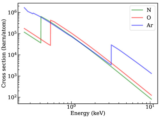
Figure 1.
X-ray cross sections of N, O, Ar in the 0.25 keV to 12 keV energy range. The K-shell absorption edges are clearly visible (0.4 keV, 0.53 keV and 3.2 keV for N, O and Ar). The cross sections at K-shell absorption edges of N, O and Ar are clearly different, which provides an opportunity to retrieve atmospheric densities of different elements.
In this work, in Equation (2) represents the atmospheric number density of N, O and Ar at the tangent point altitudes, which is calculated by the NRLMSISE-00 model. The input parameters of NRLMSISE-00 are shown in Table 1. To simulate the spectral data during occultation, noise needs to be added to the spectral forward model. Assume that the noise satisfies the Gaussian distribution of = 0 and = . As shown in Figure 2, panels (a1) and (b1) are energy spectrum models at 150 km and 185 km calculated by Equation (4), respectively, panels (a2) and (b2) are noise added to the energy spectrum models at 150 km and 185 km, respectively, and panels (a3) and (b3) represent simulation data after adding noise. Figure 2 only lists the energy spectrum at 150 km and 185 km, and the energy spectrum simulation data at other altitudes are also generated by adding corresponding noise.

Table 1.
The input parameters of NRLMSISE-00 for the calculation of atmospheric density.
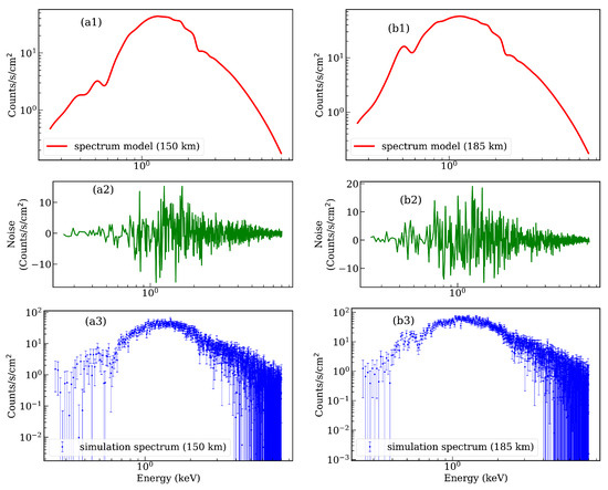
Figure 2.
Panels (a1,b1) are energy spectrum models at 150 km and 185 km, respectively, panels (a2,b2) are noise, panels (a3,b3) represent energy spectrum simulation data at 150 km and 185 km, respectively.
3. Element Density Retrieval
To retrieve the atmospheric number density of each element in the atmosphere, several parameters , and are introduced into Equation (2), the specific forms are as follows
where , and are correction factors, , and are the X-ray cross sections of N, O, and Ar, , and are the initial values of N, O and Ar number density calculated by NRLMSISE-00 in this work. Based on the input parameters in Table 1, the density values of NRLMSISE-00 in the altitude range of 10–400 km are calculated, and it is found that the density of Ar accounts for 0–0.93% of the total density. The signal to noise ratio of X-ray photon attenuation signal caused by Ar elements is very low, and the signal is almost completely submerged in noise, which leads to great uncertainty in the retrieved results of Ar element density. Therefore, the density of Ar is set to the nominal values of NRLMSISE-00 due to the limitation of signal-to-noise ratio, i.e., = 1.
By fitting the energy spectrum forward model and simulation data, the values of the correction factors and can be determined, so that the number density of N and O can be retrieved,
where is the retrieved density of N at the tangent point altitude h, and is the retrieved density of O at the tangent point altitude h.
In this work, a Bayesian estimation method is used to realize the estimation of , and B parameters. The energy spectrum model and simulation data are fitted based on Bayes’ theorem [21],
where = {}, D is the observed data, S is the model, is the posterior probability distribution, is the prior distribution, is the likelihood function and is the Bayesian evidence.
The X-ray photon count satisfies Poisson distribution, so the best way to evaluate the goodness of fit of the model is the product of Poisson probability in each bin. This is also called the likelihood function, but it is often taken in natural logarithmic form of the likelihood function for simplicity of calculation [22],
where is the observed data in the ith bin, is the ith model value.
Markov chain Monte Carlo (MCMC) algorithm is a common method to realize parameter estimation based on Bayesian inference. The posterior probability distribution of the parameters is obtained by random sampling in the probability density space using Markov chain, and the uncertainty of the parameters is evaluated [23,24,25,26].
In this work, the MCMC algorithm is implemented through the Python package emcee [27]. The posterior probability distribution of parameters is obtained by selecting 10 walkers, each with 5000 sampling points, and then burning the first 500 steps of each walker. The fitting results of , and B are shown in Table 2. It is found that there may be sharp jumps between adjacent retrieved results, for example, the corresponding to 200 km is 1.77, and the corresponding to 205 km is 0.86, which is related to the random noise added to the energy spectrum model. Because the random noise is artificially added random numbers that satisfies a certain distribution in this paper, the value of the random noise added at two adjacent altitudes may be very different from each other, so it is possible for the retrieved results to have sharp jumps. A comparison of the best fitting energy spectrum model and energy spectrum simulation data is shown in Figure 3. A comparison of the retrieved results of O and N and the NRLMSISE-00 model values is shown in Figure 4. It is found that the retrieved errors of elements N and O are small in the altitude range of 140–200 km. The retrieved error of elements N and O in the altitude range of 120–140 km is relatively large, especially for O, whose maximum error is 93.7% at 120 km, which is related to the low signal-to-noise ratio of simulation data as shown in Figure 3 and the low proportion of O element in the line of sight as shown in Table 3. Based on the number density of the NRLMSISE-00 model and onion-peeling algorithm, the proportion of the column density of elements O and N in the total column density of elements (N + O) in the line of sight in the altitude range of 120–250 km is calculated, as shown in Table 3. It is found that the O/N ratio increases with altitude above 120 km. The reason is that the probability of dissociation of O by solar ultraviolet irradiation is relatively high, the weight of atomic oxygen produced is half of the original, and the concentration decreases at a relatively small rate with the increase of altitude. N also undergoes photodissociation, but with much less probability than O, it remains mainly in molecular form at higher altitudes. As a result, heavier molecular nitrogen settles out of the atmosphere relatively quickly [28]. Eventually, the relative concentration of oxygen increases above ∼120 km and atomic oxygen become the principal constituent of the atmosphere above ∼200 km. From Table 3, it is found that the proportion of O element in line of sight in the altitude range of 120–140 km is 21.70–26.64%. Due to the low proportion of O element (refer to Table 3) and the low signal-to-noise ratio of simulation data (refer to Figure 3), the retrieved error of O element is relatively large in the altitude range of 120–140 km. In the altitude range of 200–250 km, the inconsistency between the retrieved results of elements N and O and the NRLMSISE-00 model values increases, and the error of N and O retrieved results is relatively large. This is because with the increase of altitude, the atmosphere becomes thinner, and only a few X-ray photons are absorbed by the atmosphere, most of the photons penetrate the atmosphere, increasing the uncertainty of the retrieved results [8].

Table 2.
The fitting results and confidence intervals of the correction factors , and background B.
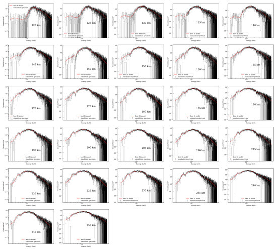
Figure 3.
Comparison of the best fitting energy spectrum model and energy spectrum simulation data in the altitude range of 120–250 km. The black dots with error bars represent the simulation data, and the solid red lines represent the best fit model. It is found that the best fit is visually in good agreement with the simulation data.
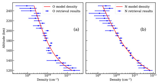
Figure 4.
Comparison between the retrieved results of elements O and N and NRLMSISE-00 model values. The blue dots with error bars represent the retrieved result of O element, and the solid red line represents the model value of O element in Panel (a). Panel (b) is the same as Panel (a) but for the N element.

Table 3.
The proportion of O and N in the line of sight at different altitudes.
4. Discussion and Summary
In this paper, we model the energy spectrum of the Crab Nebula during X-ray occultation using NICER telescope parameters, and realize the simulated verification of elements O and N density retrieval using X-ray occultation. To achieve element density retrieval, the energy band of detector needs to contain the K-shell absorption edges of elements, because there are significant differences in X-ray cross sections at the absorption edges. By fitting the energy spectrum model and simulation data in the energy range of 0.25–8 keV, the element densities of N and O in the range of 120–250 km are obtained. It is found that the retrieved error of O element is large in the altitude range of 120–140 km, which is related to the low proportion of O in the line of sight and the low signal-to-noise ratio of simulation data. In practical applications, it is necessary to select X-ray sources with stronger radiation as target sources to generate high signal-to-noise ratio signals, such as the Sun and Scorpius X–1. Figure 5 shows the comparison of the reference energy spectrum of Scorpius X–1 and the Crab Nebula, which is based on NICER parameters, and it is found that the spectral count rate of Scorpius X–1 is an order of magnitude higher than that of the Crab Nebula. In the altitude range of 200–250 km, the inconsistency between the retrieved element density and NRLMSISE-00 model values increases because very few photons are absorbed. In the future, the retrieval of element density will be realized based on the measured data of X-ray occultation.
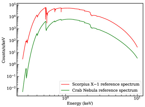
Figure 5.
Comparison of reference energy spectrum of Scorpius X–1 and the Crab Nebula. The solid red line shows the reference spectrum of Scorpius X–1 and the solid green line shows the reference spectrum of the Crab Nebula. It is found that the spectral count rate of Scorpius X–1 is about an order of magnitude higher than that of the Crab Nebula.
Author Contributions
Conceptualization, B.L.; methodology, D.Y.; software, D.Y.; validation, D.Y.; formal analysis, D.Y.; investigation, D.Y.; writing—original draft preparation, D.Y.; writing—review and editing, D.Y. and B.L.; visualization, D.Y.; supervision, B.L.; funding acquisition, B.L. All authors have read and agreed to the published version of the manuscript.
Funding
This research was funded by the National Key Research and Development Program of China (Grant No. 2017YFB0503300).
Data Availability Statement
The NICER data are available at https://heasarc.gsfc.nasa.gov/docs/nicer/nicer_archive.html (accessed on 1 August 2022). The data processing software HEAsoft6.29c is available at https://heasarc.gsfc.nasa.gov/lheasoft/download.html (accessed on 1 August 2022). The calibration files CALDBxti20170707 can be obtained at https://heasarc.gsfc.nasa.gov/docs/heasarc/caldb/nicer/ (accessed on 1 August 2022). The Python implementation of the affine-invariant ensemble sampler for MCMC emcee can be obtained at https://emcee.readthedocs.io/en/stable/ (accessed on 1 August 2022). The software XrayDB is used to obtain the X-ray cross sections of N, O and Ar in this paper can be obtained at https://xraypy.github.io/XrayDB/python.html (accessed on 1 August 2022).
Acknowledgments
D.Y. thanks Keith C. Gendreau from NASA’s Goddard Space Flight Center for a detailed email response to the X-ray occultation in the NICER observations.
Conflicts of Interest
The authors declare no conflict of interest.
Abbreviations
The following abbreviations are used in this manuscript:
| MCMC | Markov Chain Monte Carlo |
| NICER | The Neutron star Interior Composition Explorer |
| XTI | X-ray Timing Instrument |
| RSP | detector response matrix |
References
- Mori, K.; Tsunemi, H.; Katayama, H.; Burrows, D.N.; Garmire, G.P.; Metzger, A.E. An X-ray Measurement of Titan’s Atmospheric Extent from Its Transit of the Crab Nebula. Astrophys. J. 2004, 607, 1065–1069. [Google Scholar] [CrossRef]
- Rahmati, A.; Larson, D.E.; Cravens, T.E.; Lillis, R.J.; Lee, C.O.; Dunn, P.A. MAVEN SEP Observations of Scorpius X-1 X-rays at Mars: A Midatmosphere Occultation Analysis Technique. Geophys. Res. Lett. 2020, 47, e88927. [Google Scholar] [CrossRef]
- Picone, J.M.; Hedin, A.E.; Drob, D.P.; Aikin, A.C. NRLMSISE-00 empirical model of the atmosphere: Statistical comparisons and scientific issues. J. Geophys. Res. 2002, 107, 1468. [Google Scholar] [CrossRef]
- Determan, J.R.; Budzien, S.A.; Kowalski, M.P.; Lovellette, M.N.; Ray, P.S.; Wolff, M.T.; Wood, K.S.; Titarchuk, L.; Bandyopadhyay, R. Measuring atmospheric density with X-ray occultation sounding. J. Geophys. Res. 2007, 112, A06323. [Google Scholar] [CrossRef]
- Roble, R.G.; Dickinson, R.E. How will changes in carbon dioxide and methane modify the mean structure of the mesosphere and thermosphere? Geophys. Res. Lett. 1989, 16, 1441–1444. [Google Scholar] [CrossRef]
- Katsuda, S.; Fujiwara, H.; Ishisaki, Y.; Yoshitomo, M.; Mori, K.; Motizuki, Y.; Sato, K.; Tashiro, M.S.; Terada, Y. New Measurement of the Vertical Atmospheric Density Profile from Occultations of the Crab Nebula With X-ray Astronomy Satellites Suzaku and Hitomi. J. Geophys. Res. 2021, 126, e28886. [Google Scholar] [CrossRef]
- Yu, D.; Li, H.; Li, B.; Ge, M.; Tuo, Y.; Li, X.; Xue, W.; Liu, Y.; Wang, A.; Zhu, Y.; et al. Measurement of the vertical atmospheric density profile from the X-ray Earth occultation of the Crab Nebula with Insight-HXMT. Atmos. Meas. Tech. 2022, 15, 3141–3159. [Google Scholar] [CrossRef]
- Yu, D.; Li, H.; Li, B.; Ge, M.; Tuo, Y.; Li, X.; Xue, W.; Liu, Y. New method for Earth neutral atmospheric density retrieval based on energy spectrum fitting during occultation with LE/Insight-HXMT. Adv. Space Res. 2022, 69, 3426–3434. [Google Scholar] [CrossRef]
- Gendreau, K.C.; Arzoumanian, Z.; Adkins, P.W.; Albert, C.L.; Anders, J.F.; Aylward, A.T.; Baker, C.L.; Balsamo, E.R.; Bamford, W.A.; Benegalrao, S.S.; et al. The Neutron star Interior Composition Explorer (NICER): Design and development. In Space Telescopes and Instrumentation 2016: Ultraviolet to Gamma Ray; Society of Photo-Optical Instrumentation Engineers (SPIE) Conference Series; den Herder, J.W.A., Takahashi, T., Bautz, M., Eds.; SPIE: Bellingham, WA, USA, 2016; Volume 9905, p. 99051H. [Google Scholar] [CrossRef]
- Russell, J.M.; Gordley, L.L.; Park, J.H.; Drayson, S.R.; Hesketh, W.D.; Cicerone, R.J.; Tuck, A.F.; Frederick, J.E.; Harries, J.E.; Crutzen, P.J. The Halogen Occultation Experiment. J. Geophys. Res. 1993, 98, 10777–10797. [Google Scholar] [CrossRef]
- Lumpe, J.D.; Floyd, L.E.; Herring, L.C.; Gibson, S.T.; Lewis, B.R. Measurements of thermospheric molecular oxygen from the Solar Ultraviolet Spectral Irradiance Monitor. J. Geophys. Res. 2007, 112, D16308. [Google Scholar] [CrossRef]
- Noël, S.; Bramstedt, K.; Rozanov, A.; Bovensmann, H.; Burrows, J.P. Water vapour profiles from SCIAMACHY solar occultation measurements derived with an onion peeling approach. Atmos. Meas. Tech. 2010, 3, 523–535. [Google Scholar] [CrossRef]
- Li, X.; Li, X.; Tan, Y.; Yang, Y.; Ge, M.; Zhang, J.; Tuo, Y.; Wu, B.; Liao, J.; Zhang, Y.; et al. In-flight calibration of the Insight-Hard X-ray Modulation Telescope. J. High Energy Astrophys. 2020, 27, 64–76. [Google Scholar] [CrossRef]
- Kirsch, M.G.; Briel, U.G.; Burrows, D.; Campana, S.; Cusumano, G.; Ebisawa, K.; Freyberg, M.J.; Guainazzi, M.; Haberl, F.; Jahoda, K.; et al. Crab: The standard X-ray candle with all (modern) X-ray satellites. In UV, X-ray, and Gamma-ray Space Instrumentation for Astronomy XIV; Society of Photo-Optical Instrumentation Engineers (SPIE) Conference Series; Siegmund, O.H.W., Ed.; SPIE: Bellingham, WA, USA, 2005; Volume 5898, pp. 22–33. [Google Scholar] [CrossRef]
- Meyer, M.; Horns, D.; Zechlin, H.S. The Crab Nebula as a standard candle in very high-energy astrophysics. Astron. Astrophys. 2010, 523, A2. [Google Scholar] [CrossRef]
- Yan, L.L.; Ge, M.Y.; Lu, F.J.; Zheng, S.J.; Tuo, Y.L.; Li, Z.J.; Song, L.M.; Qu, J.L. Time Evolution of the X-ray and ɤ-ray Fluxes of the Crab Pulsar. Astrophys. J. 2018, 865, 21. [Google Scholar] [CrossRef]
- Arnaud, K.; Dorman, B.; Gordon, C. XSPEC: An X-ray Spectral Fitting Package; Astrophysics Source Code Library: Houghton, MI, USA, 1999. [Google Scholar]
- Massaro, E.; Campana, R.; Cusumano, G.; Mineo, T. The optical to ɤ-ray emission of the Crab pulsar: A multicomponent model. Astron. Astrophys. 2006, 459, 859–870. [Google Scholar] [CrossRef]
- Chantler, C. Detailed Tabulation of Atomic Form Factors, Photoelectric Absorption and Scattering Cross Section, and Mass Attenuation Coefficients in the Vicinity of Absorption Edges in the Soft X-ray (Z = 30–36, Z = 60–89, E = 0.1 keV–10 keV), Addressing Convergence Issues of Earlier Work. J. Synchrotron Radiat. 2001, 8, 1124. [Google Scholar] [CrossRef]
- Elam, W.; Ravel, B.; Sieber, J. A new atomic database for X-ray spectroscopic calculations. Radiat. Phys. Chem. 2002, 63, 121–128. [Google Scholar] [CrossRef]
- Bayes, M.; Price, M. An Essay towards Solving a Problem in the Doctrine of Chances. By the Late Rev. Mr. Bayes, FRS Communicated by Mr. Price, in a Letter to John Canton, AMFRS. Philos. Trans. R. Soc. Lond. Ser. I 1763, 53, 370–418. [Google Scholar]
- Cash, W. Parameter estimation in astronomy through application of the likelihood ratio. Astrophys. J. 1979, 228, 939–947. [Google Scholar] [CrossRef]
- Chib, S.; Greenberg, E. Understanding the Metropolis-Hastings Algorithm. Am. Stat. 1995, 49, 327–335. [Google Scholar] [CrossRef]
- Dunkley, J.; Bucher, M.; Ferreira, P.G.; Moodley, K.; Skordis, C. Fast and reliable Markov chain Monte Carlo technique for cosmological parameter estimation. Mon. Not. R. Astron. Soc. 2005, 356, 925–936. [Google Scholar] [CrossRef]
- Sharma, S. Markov Chain Monte Carlo Methods for Bayesian Data Analysis in Astronomy. Annu. Rev. Astron. Astrophys. 2017, 55, 213–259. [Google Scholar] [CrossRef]
- Lamminpää, O.; Hobbs, J.; Brynjarsdóttir, J.; Laine, M.; Braverman, A.; Lindqvist, H.; Tamminen, J. Accelerated MCMC for Satellite-Based Measurements of Atmospheric CO2. Remote Sens. 2019, 11, 2061. [Google Scholar] [CrossRef]
- Foreman-Mackey, D.; Hogg, D.W.; Lang, D.; Goodman, J. emcee: The MCMC Hammer. Publ. Astron. Soc. Pac. 2013, 125, 306. [Google Scholar] [CrossRef]
- Ortner, J.; Maseland, H. Introduction to Solar Terrestrial Relations: Proceedings of the Summer School in Space Physics Held in Alpbach, Austria, July 15–August 10, 1963 and Organized by the European Preparatory Commission for Space Research (COPERS); Springer Science & Business Media: Berlin, Germany, 2012; Volume 2. [Google Scholar]
Publisher’s Note: MDPI stays neutral with regard to jurisdictional claims in published maps and institutional affiliations. |
© 2022 by the authors. Licensee MDPI, Basel, Switzerland. This article is an open access article distributed under the terms and conditions of the Creative Commons Attribution (CC BY) license (https://creativecommons.org/licenses/by/4.0/).