Using UAV to Identify the Optimal Vegetation Index for Yield Prediction of Oil Seed Rape (Brassica napus L.) at the Flowering Stage

Abstract

Suitability of the vegetation indices of normalized difference vegetation index (NDVI), blue normalized difference vegetation index (BNDVI), and normalized difference yellowness index (NDYI) obtained by means of UAV at the flowering stage of oil seed rape for the prediction of seed yield and usability of these vegetation indices in the identification of anomalies in the condition of the flowering growth were verified based on the regression analysis. Correlation analysis was performed to find the degree of yield dependence on the values of NDVI, BNDVI, and NDYI indices, which revealed a strong, significant linear positive dependence of seed yield on BNDVI (R = 0.98) and NDYI (R = 0.95). The level of correlation between the NDVI index and the seed yield was weaker (R = 0.70) than the others. Regression analysis was performed for a closer determination of the functional dependence of NDVI, BNDVI, and NDYI indices and the yield of seeds. Coefficients of determination in the linear regression model of NDVI, BNDVI, and NDYI indices reached the following values: R² = 0.48 (NDVI), R² = 0.95 (BNDVI), and R² = 0.90 (NDYI). Thus, it was shown that increased density of yellow flowers decreased the relationship between NDVI and crop yield. The NDVI index is not appropriate for assessing growth conditions and prediction of yields at the flowering stage of oil seed rape. High accuracy of yield prediction was achieved with the use of BNDVI and NDYI. The performed analysis of NDVI, BNDVI, and NDYI demonstrated that particularly the BNDVI and NDYI indices can be used to identify problems in the development of oil seed rape growth at the stage of flowering, for their precise localization, and hence to targeted and effective remedial measures in line with the principles of precision agriculture.

1. Introduction

The last twenty years recorded a significant development of unmanned aerial vehicles (UAVs) or drones in a range of applications such as observation, geographical studies, monitoring of fires, safety, military applications, search and rescue, or agriculture [1]. In agriculture, remote sensing by UAV appeared as very effective in the assessment of the condition of crops. Compared for example with satellite imagery, UAV monitoring features a greater accuracy of measured data [1]. The development of small multi-rotor UAV systems is provided by their portability, low purchasing price, maneuverability, and simple use [2].

Unmanned aerial vehicles surpass manned aerial vehicles in the versatility of use, in cost, and in the capacity of reaching finer time and space resolution [3]. Lower flight altitude of UAV allows to use cheaper sensors compared with those that are necessary in piloted aircrafts without disturbing the upper storey of monitored crops when flying. Moreover, the speed of deployment and possibility of data collection are useful in inaccessible areas such as waterlogged lands [4].

Yang and Hoffmann [5] mentioned other advantages of UAV compared with satellite systems such as remote sensing of Earth platforms. These include easy deployment, availability of images for visual assessment almost in real time and overcoming of weather limitations especially as far as cloudiness is concerned. The authors also pointed out that satellite images of required target areas cannot be taken always in the necessary time due to limitations connected with satellite orbits.

The above pros predetermine the UAV for use in precision agriculture which also recorded a significant progress in recent years [6]. There is a number of various UAV applications in this field mentioned in literature.

One of them is the monitoring of crops by means of high-resolution multispectral images. This is how various vegetation indices (VIs) can be determined, which can be used to assess the condition of plant biomass [7], to localize weeds [8], pests, diseases [9,10], to establish nutrient requirements [7], to estimate yields [11], or to identify drought stress [12]. Based on the obtained information, efficient measures with the use of agrochemicals can be implemented at a given site, at a given time and in an optimum amount [13,14], thus saving agricultural inputs, mitigating environmental impacts, and increasing profits. UAV are selected as an option to satellite remote sensing because of their spatial and temporal resolution. However, some technical aspects can be improved to increase efficiency in precision agriculture and to evaluate economic benefits of UAV application at a farm-scale level [2]. Moreover, law restrictions of UAV operation by governments need to be considered for their utilization in precision farming.

Matese et al. [3] compared the normalized difference vegetation index (NDVI) obtained from three different platforms: satellite, manned aircraft, and UAV in order to evaluate possibilities of each platform in the characterization of spatial variability of experimental vineyard. The authors found out that due to their coarser spatial resolution, satellite images cannot adequately represent variability inside the vineyard with a higher heterogeneity, and based on this finding, they concluded that UAV is suitable for relatively smaller plots and that the breaking point occurs around an area of five hectares. In larger areas, other platforms appear as more advantageous.

Oil seed rape (Brassica napus L.; OSR) is one of the most important crops in the world for human consumption, a source for meal with a high content of proteins to feed farm animals, and a renewable biological raw material for chemical and oil industry [15]. Yield components of OSR include the number of pods, the number of seeds in the pod, and the weight of one seed [16].

OSR passes through three different morphological forms during its development. At the first stage, the growth is dominated by leaves, at the second stage, the growth features yellow petals, and at the third stage, the growth forms stems and pods. Each form of the growth strongly affects the mode of solar radiation interception [17]. Plants such as wheat and maize with inconspicuous flowers simply become green upon entering the reproduction growth stages, and yellow or even brown when they ripen [11]. Many oil crops of Brassica genus, however, become green and then yellow due to the occurrence of conspicuous yellow flowers, with the green and the yellow overlapping when the growth ripens. This time-spectral variability deserves a very careful consideration when selecting a spectral index that should correlate with the physiologically significant variable such as the yield of seeds [11]. The time-spectral variability is a function of the morphological development of OSR.

One of the most used vegetation indices is the normalized difference vegetation index (NDVI) that combines two of the most important agronomic parameters: the status of plants (occurrence of stress) and the amount of biomass on the unit area. NDVI is also used to distinguish vegetation from non-vegetation areas. Values of NDVI were found to be higher in agricultural areas than in forest areas, while water surfaces provided minus NDVI values [18]. As it correlates well with the photosynthetic capacity, NDVI theoretically provides effective yield estimates [19].

Another used vegetation index is the blue normalized difference vegetation index (BNDVI) which is an index without red channel availability that uses the visible blue for areas sensitive to chlorophyll content. It provides the ratio between the near infrared (NIR) and the blue zone of the spectrum, which strongly correlates with the leaf area index (LAI) [20].

Sulik and Long [21] suggested a normalized difference yellowness index (NDYI) determining a normalized ratio between the Green and the Blue zone. It was proposed in order to estimate the number of flowers in OSR and other yellow-flowering plants and hence to derive the vegetation cover density. Production of OSR flowers plays an important role in yield prediction, and the yellowness of OSR petals can be a critical reflective signal and a good predictor of the number of pods, and hence the yield of seeds [16]. It is a known fact that yellow flowers increase reflectance of green color while slightly decreasing reflectance of blue color [22]. Therefore, the blue zone is a good denominator for the index of flower variability, the value of which increases with the increasing reflectance in the green zone. For the numerator, the green zone is a better choice than the red zone because the red color reflectance changes with the content of chlorophyll which changes with the displacement of soluble photosynthate by healthy leaves into buds and flowers [23,24]. This is why the ratio of blue and green light should be functioning properly for the estimate of yellowness as it changes in opposite directions due to the presence of yellow flowers. The green/blue ratio values should have a positive relation to the density of flowers while the NDVI values decrease with the increasing coverage of flowers [23].

It was also found [24] that NDYI is the most useful index of all studied VI for the monitoring of changes in the content of chlorophyll in leaves as well as the greenness of rice leaves during the entire period of growth.

The relationship between some VI and OSR yields was studied already by many authors [16,25,26,27]. New benefits of this research are proposals of prediction models based on which future OSR yields can be estimated with high accuracy at the stage of flowering even in the conditions of high variability of above-ground and under-ground vegetation environments caused by various biotic and abiotic stresses.

The goal of this study was to verify, on the basis of regression models, the suitability of NDVI, BNDVI, and NDYI vegetation indices obtained by means of UAV at the stage of flowering for predicting the OSR yield, and the usability of the vegetation indices for the identification of anomalies in the condition of the flowering OSR growth, these being the initial phases of a long-term field experiment focused on vegetation indices potentially applicable in studying winter OSR at the stage of flowering.

2. Materials and Methods

2.1. Field Experiment Localization

The experimental plot (Figure 1) is situated not far from the research station of Agricultural Research Institute in Troubsko (Czech Republic, 49.1688878°N, 16.4948747°E). In 2018, a precrop on the plot was winter wheat. The experiment was established in 2019. In terms of agro-ecological classification, the plot is situated in the region typical of growing root crops (e.g., sugar beet), in the mildly warm and mildly dry climatic zone, at an altitude of 290 m a.s.l., with a mean annual temperature of 8.95 °C and a long-term annual total precipitation amount of 525.6 mm (the values correspond to the 1981–2010 climatic normal). According to the Köppen climate classification, it is the warm summer humid continental climate DfB. Geological bedrock is loess and loess loam of the Bohemian Massif, according to the World Reference Base (international standard for soil classification system) [28], the soil type was determined as Haplic Luvisol. Meteorological and climatological parameters are shown in

Table 1. Weather conditions at the Troubsko field experimental station, 2019 and 2020. Average monthly temperatures and mean annual precipitation amounts for long-term standard (1981–2010). Meteorological data for individual months were measured by a professional weather station (ID: B2TROU01; type: AKS2) operated by the Czech Hydrometeorological Institute (Ministry of the Environment of CZE). The long-term standards for Troubsko area were calculated on the basis of data from 1981 to 2010 (data provider: Czech Hydrometeorological Institute; https://www.chmi.cz/historicka-data/pocasi/zakladni-informace?l=en) (accessed on 1st May 2022).

Year	Total Month Precipitation												Total Amount
	8	9	10	11	12	1	2	3	4	5	6	7	Vegetation Period
2019–2020	55.9	72.6	60.4	40.1	42.9	8.5	27.1	25.7	20.3	65.4	87.2	59.0	565.1
1981–2010	63.7	48.2	32.1	36.4	32.0	25.0	23.9	31.5	32.0	60.5	68.7	71.6	525.6
Year	Average month temperature												Average
	8	9	10	11	12	1	2	3	4	5	6	7	vegetation period
2019–2020	20.8	14.6	9.9	5.2	0.6	−0.2	4.6	5.3	9.9	12.6	18.0	19.2	10.0
1981–2010	18.8	14.1	8.8	3.5	−0.6	−1.7	−0.3	3.8	9.5	14.6	17.4	19.5	9.0

.

2.2. Establishment and Harvest of the Experiment

OSR was sown on 29 August 2019 using a waste-less seed drill on 80 plots sized 8.0 × 1.25 m. The experiment was based on an area of 33 × 41 m (1353 m²) and was established in four replications. In each replication, 20 variants of fertilization were applied before the sowing. The effect of fertilization on the crop development and yield level was not evaluated within this study, only the relationship between yield and spectral properties of vegetation was analyzed. As the goal of this study was the identification of potential spatial variability in the condition of the flowering growth based on VI and verification of the relation between VI and yields, the effect of different fertilization variants on the values of VI and yields was not assessed. Experiment randomization is illustrated in Figure 2. In the experiment, OSR of Kuga variety was sown. The seed was treated with the Cruiser OSD mordant at 15 l/t, sowing rate was 3.5 kg/ha, and distance between the rows was 12.5 cm, sowing depth 2–3 cm. Boundaries of the experimental site were sighted using the real-time kinematic (RTK) Global navigation satellite system (GNSS) receiver, and individual plots were aligned using the geographical information system (GIS) ESRI ArcGIS.

The experiment was harvested on 24 July 2020 by the Sampo combine harvester. The individual experimental plots were harvested separately and seed yields from each plot were recorded.

2.3. Vegetation Indices

Images of the experimental growth of winter OSR at the stage of full flowering BBCH 65 [29] were taken for complex mapping of the experiment on 1 May 2020 using UAV DJI Matrice M600 (Figure 3) and multispectral camera Micasense Altum (captures six bands: red, green, blue, red edge, near-infrared, and thermal). The camera takes images in 6 narrow spectral bands: blue (center wavelength 475 nm), green (560 nm), red (668 nm), red-edge (717 nm), near-infrared NIR (842 nm), and long-wave infrared LWIR (11 µm). Simultaneously the incoming radiation intensity is recorded by the Micasense DLS2 sensor installed on the upper part of the drone for the normalization of incoming light conditions. The drone was moving at a flight altitude of 25 m, and the sensor resolution of 2064 × 1544 (3.2 MPx) provided images with ground sample distance (GSD) = 1.08 cm. Radiometric calibration of the multispectral camera was ensured by scanning the spectral panel Micasense CRP and using procedures recommended by the manufacturer. Geometric accuracy of acquired images was guaranteed by RTK used in the guidance system of the drone and by the placement of 4 ground control points (GCP) in the observed area.

The orthomosaic of spectral bands was created using the Agisoft Metashape software together with the calculation of the digital surface model (DSM). The radiometric calibration of the sensor was followed by the conversion of digital values of the orthomosaic to the values of surface spectral reflectance by Micasense calibration panel. As the next step, the combined multispectral orthomosaic with all spectral bands was created, from which then three vegetation indices(NDVI, BNDVI, and NDYI) were calculated according to Equations (1)–(3) (

Table 2. Vegetation indices used.

Equation (1) [30]	Normalized difference vegetation index (NDVI)
	NDVI =	RNIR – RRed
		RNIR + RRed
Equation (2) [20]	Blue normalized difference vegetation index (BNDVI)
	BNDVI =	RNIR – Rblue
		RNIR + Rblue
Equation (3) [21]	Normalized difference yellowness index (NDYI)
	NDYI =	Rgreen – Rblue
		Rgreen + Rblue

Where R_NIR, R_red, R_green, and R_blue are the reflectance values at Micasense Altum spectral bands centered on 842, 668, 560, and 475 nm, respectively.

). The index multispectral map serves to illustrate the condition of crop growth. The data were converted to the GIS software, (ESRI ArcGIS), where mean values of vegetation indices were determined for the individual plots (Figure 2) using zonal statistics tool. The assessed surface area of the plots was reduced on all sides in order to eliminate marginal effects of lanes.

2.4. Weather Conditions in 2019–2020

Compared with the standard, the period from the sowing to the end of 2019 (August–December) recorded the above-average precipitation (+28%). Air temperatures in this period were by 1.3 °C higher than the long-term average (Table 2).

Compared with the long-term average, the period from the beginning of 2020 (January–July) to the harvest was slightly below average in terms of precipitation (−6%). During the first seven months of the year, air temperatures were slightly above the standard. The greatest difference between the monthly temperature average and the long-term average was recorded in February (+4.9 °C). In contrast, at the time of OSR flowering in May, the average temperature ranged more than 2 °C below the standard (Table 2).

2.5. Statistical Analysis—Data Treatment

The results were statistically processed using the Statistica 14 software (TIBCO Software Inc., Palo Alto, CA, USA). Based on the exploratory data analysis (EDA), remote data were identified. Tukey’s HSD test was performed to confirm or exclude possible significant differences within the respective vegetation indices (VI) and in the yields of seeds between the respective experimental plots (p < 0.05). In addition, Pearson’s correlation analysis was performed of seed yields and NDVI, BNDVI, and NDYI indices in order to establish the degree of interdependence (p < 0.05). Finally, regression analysis was computed, and regression models were constructed on the basis of which the degree was established to which the studied VI explain the variability of yields and whether the indices can be used to predict yields at the stage of flowering. Applicability of VI for the identification of anomalies in the condition of OSR flowering growth was verified using visualization by means of contour maps compiled on the basis of detected VI values and OSR yields reached.

3. Results and Discussion

3.1. Vegetation Indices (VI)

Figure 4a shows the experimental growth of OSR in four replications at the flowering stage (Figure 4). Red color in Figure 4b (red channel negative) shows gaps in the growth, created by weeds, non-flowering, or missing OSR plants.

Graphical illustration of NDVI, BNDVI and NDYI vegetation indices and differences in capturing crop density in the field trial is presented in Figure 5, Figure 6 and Figure 7. Furthermore, results of the statistical analysis of individual vegetation indices and yield are shown in

Table 3. Results of the statistical analysis of vegetation indices and yield.

Variable	Mean	SD	N	Minimum	Maximum	Span
NDVI	0.63	0.02	80.00	0.57	0.67	0.10
BNDVI	0.86	0.02	80.00	0.81	0.89	0.08
NDYI	0.57	0.04	80.00	0.47	0.63	0.16
YIELD	3.79 *	0.38	77 *	2.81	4.40	1.58

* Without outlier values.

.

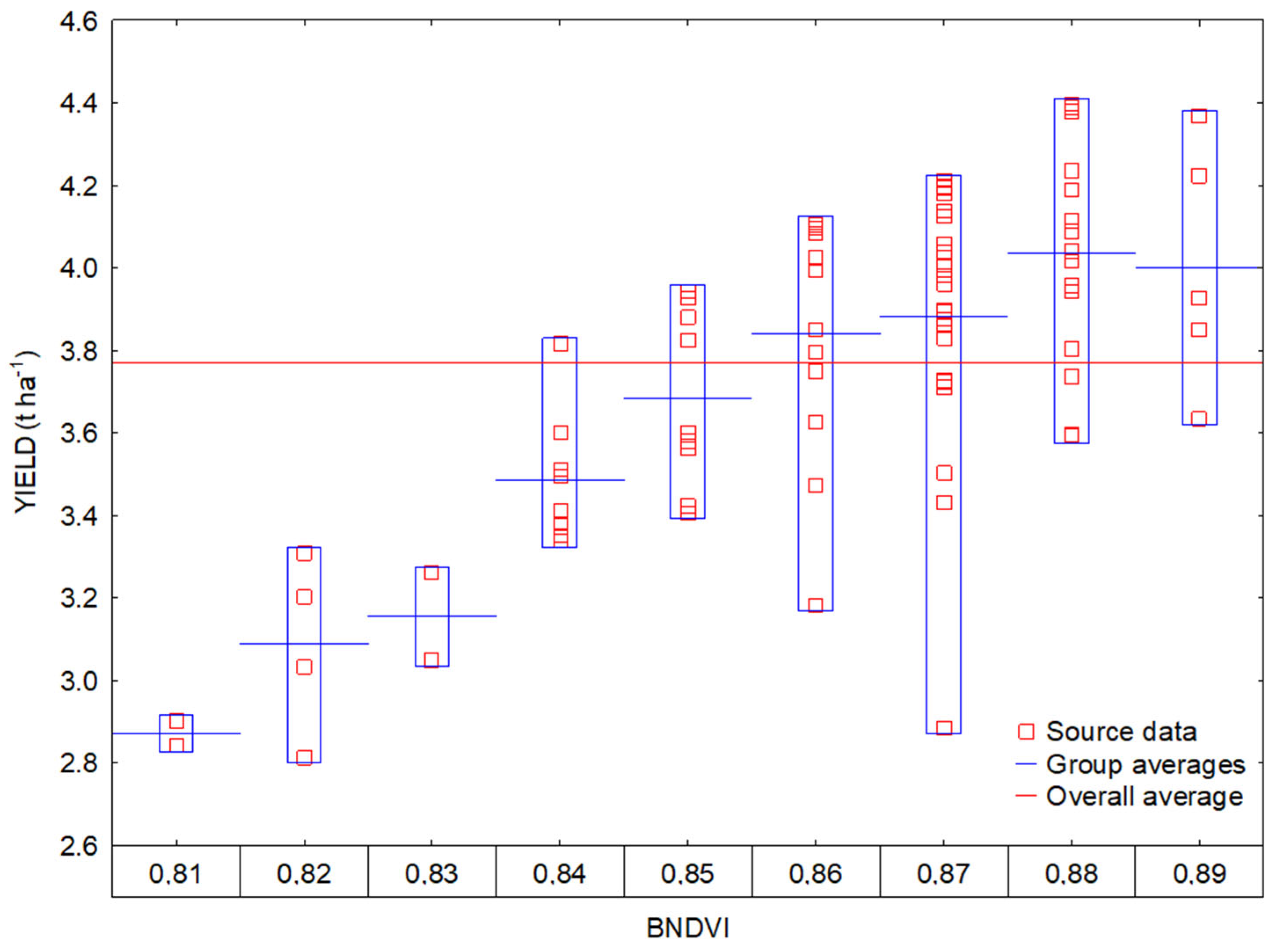
3.2. Interactions between Vegetation Indices and Yields

Possible mutual correlations of vegetation indices and dependence of yield on the values of NDVI, BNDVI, and NDYI indices were established by correlation analysis (

Table 4. Summary of correlations (Pearson’s correlation coefficient R) among the measured variables.

Variable	NDVI	BNDVI	NDYI	YIELD (t/ha)
NDVI	1.00	0.65	0.39	0.47
BNDVI	0.65	1.00	0.92	0.80
NDYI	0.39	0.92	1.00	0.84
YIELD (t/ha)	0.47	0.80	0.84	1.00

Red numerals show statistically significant correlations at a level of significance of p < 0.05.

).

Seed yields of individual plots ranged from 2.81 to 4.40 t/ha, an average yield of the whole experiment was 3.77 t/ha. The correlation analysis indicates that the yield of seeds exhibits a strong, significant, and linear positive dependence on the NDYI (R = 0.84) and BNDVI (R = 0.80) indices. The correlation between the NDVI index and yield was weaker (R = 0.47). As NDVI exhibits strong correlations with the crop yields based on the maximum green leaf biomass, the relationship can be used for the determination of yield parameters (e.g., in corn) [31] or for the prediction of yield in cereals [32]. In contrast, NDYI and BNDVI were tested for the prediction of yield not only in cereals but also in oil crops. It was demonstrated during the testing that the highest values of dependence were recorded at the stage of flowering, similarly as in our experiment [11,32,33].

Hodge et al. [33] who compared the growth of OSR with the protective vegetation belts of natural or artificial origin with a control growth without the protective belt recorded only a very weak negative correlation (R = −0.37) between NDVI and yield in the control, and a strong negative correlation (R = −0.71) in the variant with the natural protective belt.

In experiments conducted by Hodge et al. [33], a negative correlation was contrarily observed between BNDVI and yield (R = −0.80).

Based on their research, Zhang et al. [16] reported that NDYI is a useful VI to express the OSR yellowness which relates to the intensity of its flowering at the stage of full bloom. The coefficient of determination (R2) identified by them ranged from 0.54 to 0.95, thus being significant and confirming the possibility of using NDYI in the prediction of yield. The measured values of NDYI (Table 3) exhibited a variance from 0.47 to 0.63, which might have been caused by the intensity of flowering. In their study, d’Andrimont et al. [34] informed that the NDYI value can be used to determine the stage of flowering or to predict yields [11]. The stage of flowering ranges from BBCH 60 (beginning of flowering) to BBCH 69 (end of flowering) with the NDYI value increasing from the BBCH 60 stage and culminating at BBCH 65/67 [34]. This may influence the measured NDYI values and cause their certain variance. The NDYI values (Table 3, Figure 7) were measured during the peak of the flowering stage (BBCH 65); however, with respect to the amount of monitored plots, some parts of the stands might have been slightly before or beyond the flowering peak, which affected the range of measured values [11,34].

3.3. Regression Analysis of Vegetation Indices and Yield

Regression analysis was performed to determine closer the functional dependence of NDVI, BNDVI, and NDYI indices and the seed yield. First, the individual measured VI values were allocated plot yields with the same VI value (Figure 8, Figure 9 and Figure 10). For each value in the interval of measured values of the respective VI, an average yield was calculated from the yields of plots with the same value of VI, i.e., for NDVI, BNDVI, and NDYI. Based on these values of VI and average yields allocated to the individual VI values, linear regression models were constructed (Figure 11, Figure 12 and Figure 13). The models illustrate the yields observed and the yields predicted based on the regression analysis of vegetation indices and yields achieved. The crop yield values achieved from the field experiment ranged from 2.81 to 4.40 t/ha. The low range of recorded yields partly limits the usage of prediction model for yield levels below the recorded minimum values. However, this yield range corresponds to the average seed yield of OSR in the Czech Republic in recent years. Further research will be conducted to increase the model reliability by extending the field trials over various soil productivity conditions and by implementing year variability.

By this method it was possible to increase the share of yield variability explained by the model compared with the procedure in which the correlation and determination coefficients were calculated from the yield of each plot (

Table 5. Comparison of correlation coefficients (R), coefficients of determination (R²) and Root Mean Square Error (RMSE) of NDVI, BNDVI, and NDYI vegetation indices and yields in different methods of calculation.

Method of Calculation	From Yields of All Plots			From Average Yields of Plots with the Same Value of VI
Parameter	NDVI	BNDVI	NDYI	NDVI	BNDVI	NDYI
Correlation coefficient R	0.47	0.80	0.84	0.70	0.98	0.95
Determination coefficient R2	0.22	0.64	0.70	0.48	0.95	0.90
RMSE (t/ha)	0.32	0.22	0.21	0.27	0.10	0.13

) in four replications. It follows from the analysis of residues that all three VI exhibited reduced accuracy of yield prediction in the lowest and highest values of the VI scale. In these marginal values, the observed yields were usually lower than the predicted yields. In the middle part of the VI scale, the residues were largely positive, which indicated that the observed yields were usually slightly higher than the predicted yields (Figure 11, Figure 12 and Figure 13). The anomalies were likely to be caused by the distribution of data entering the analysis: by the low frequency of low and high VI values and yields corresponding to them, as well as by the high frequency of mean VI values and corresponding yields (Figure 8, Figure 9 and Figure 10). NDVI was the vegetation index most affected by these anomalies. Besides the effect of the data set distribution, it can be related to the influence of biomass on the NDVI values and its lower sensitivity to the number of flowering pods. The origin of this anomaly cannot be determined with certainty based on the measured values. For example, in their 20-year study Barbosa et al. [35] recorded severe oscillations of NDVI values in dependence on the development of vegetation, but also on latitude and climatic conditions affecting vegetation. The values of NDVI and other VI were determined at the peak of vegetation during OSR flowering (BBCH 65) on the individual experimental plots. The values oscillated probably due to different properties of those plots (soil conditions and fertilization methods) that might have affected the development of the studied crop and hence also spectral characteristics of the stand [36].

Index NDVI (Figure 11) acquired values ranging from 0.57 to 0.67 (Table 3). When it increased by 0.01, the predicted yield increased by 0.07 t/ha. Differences between the predicted and actual yield values ranged from −0.53 to 0.25 t/ha. The greatest difference between the predicted and actual yield was −0.53 t/ha; it was recorded in the highest value of NDVI (0.67).

The coefficient of determination reached a value of R² = 0.48 for NDVI index at linear trend line (Figure 11) and thus it can be stated that the NDVI index explains the variability of yield variable only at 48% in this model. The reason is the fact that the OSR growth was at the stage of flowering when the images were taken. It is known that the value of NDVI decreases with the increasing density of yellow flowers [11,21]. Regarding the fact that the NDVI index is based on spectral features of plant cover, it may be less accurate in estimating above-ground biomass if there are mixed signals of flowers in the plant cover [37].

At the flowering stage, the interception of photosynthetically active radiation is reduced [22]. Yellow flowers contribute to the growth signal with the red light and this additional radiation reduces the values of NDVI [23,38,39], which affects negatively the informative capacity of NDVI in mapping biomass variability [37] or yield potential.

Sulik and Long [11,21] informed that the yellow color of OSR petals is caused by carotenoids in them absorbing the blue light, and this is why they reflect a mixed green and red light that we perceive as yellow. Compared with a growth at vegetative stage, a flowering growth reflects more and absorbs less in the range from 500 nm to 700 nm, reflecting less and absorbing somewhat more in the range from 400 nm to 500 nm at vegetative stage [22]. It has little influence on red edge or NIR [40]. This is how the red light reduces NDVI values and unfavorably affects the capacity of NDVI to reflect the growth stage and to estimate yield at the stage of flowering [11,21,23,37]. Instead of NDVI, Fan et al. [41] recommend building the prediction of OSR only on the reflectance of NIR band.

Similarly, Piekarczyk [39] claimed that the relation between NDVI and yield weakens with the increasing number of flowers. Despite this distortion caused by flowering, it is possible to state that the NDVI vegetation index captures a similar trend in the status of the winter OSR as the BNDVI and NDYI vegetation indices; predicted yield is underestimated, though.

Index BNDVI (Equation (2)) acquired values ranging from 0.81 to 0.89 (Table 3). When it increased by 0.01, the predicted yield increased by 0.15 t/ha. The greatest differences between the predicted and actual yields were −0.14 t/ha for BNDVI = 0.89 and 0.16 t/ha for BNDVI = 0.86. The coefficient of determination R² = 0.96 for index BNDVI (Figure 12) is relatively high, and thus it can be presumed that the BNDVI index explains the variability of yield variable at 96% in this model. The reason for using BNDVI is that the blue light absorbs chlorophyll but is less affected by the light reflected from yellow flowers, and thus should be a good alternative to NDVI; moreover, changes in NIR should precisely correspond to changes in the amount of vegetation, and the blue denominator should allow the ratio to correspond to such changes without being as distorted by yellow flowers as the red band [20,21].

Index NDYI Equation (3) acquired values from 0.47 to 0.63 (Table 3). When it increased by 0.01, the predicted yield increased by 0.08 t/ha. The greatest differences between the predicted and actual yields were −0.26 t/ha for NDYI = 0.48 and 0.20 t/ha for NDYI = 0.51. As the coefficient of determination R² = 0.90 for index NDYI (Figure 13) is relatively high, it can be stated that the NDYI index explains the variability of yield variable at 90% in this model.

Sulik and Long [11] stated that NDYI requires only wave bands in the visible area of the spectrum and can be therefore used for any satellite or aerial sensor with green and blue channels. This is why they used the findings to note the advantage of using the spectral index which is sensitive to the reproductive vegetation growth rather than to the vegetative growth of crops with spectrally distinctive reproductive elements of vegetation. Usage of UAV equipped with visible cameras also makes the crop survey more affordable for farming purposes in comparison with the multispectral sensors. Our research results are in line with the results published by Sulik and Long [11] who also confirmed that at the stage of flowering, NDYI is a better indicator of yield potential than NDVI. Compared with BNDVI (0.81–0.89) and NDVI (0.57–0.67), the wider range of NDYI values (0.47–0.63) in our experiment allowed a more detailed assessment of the crop growth flowering density and status.

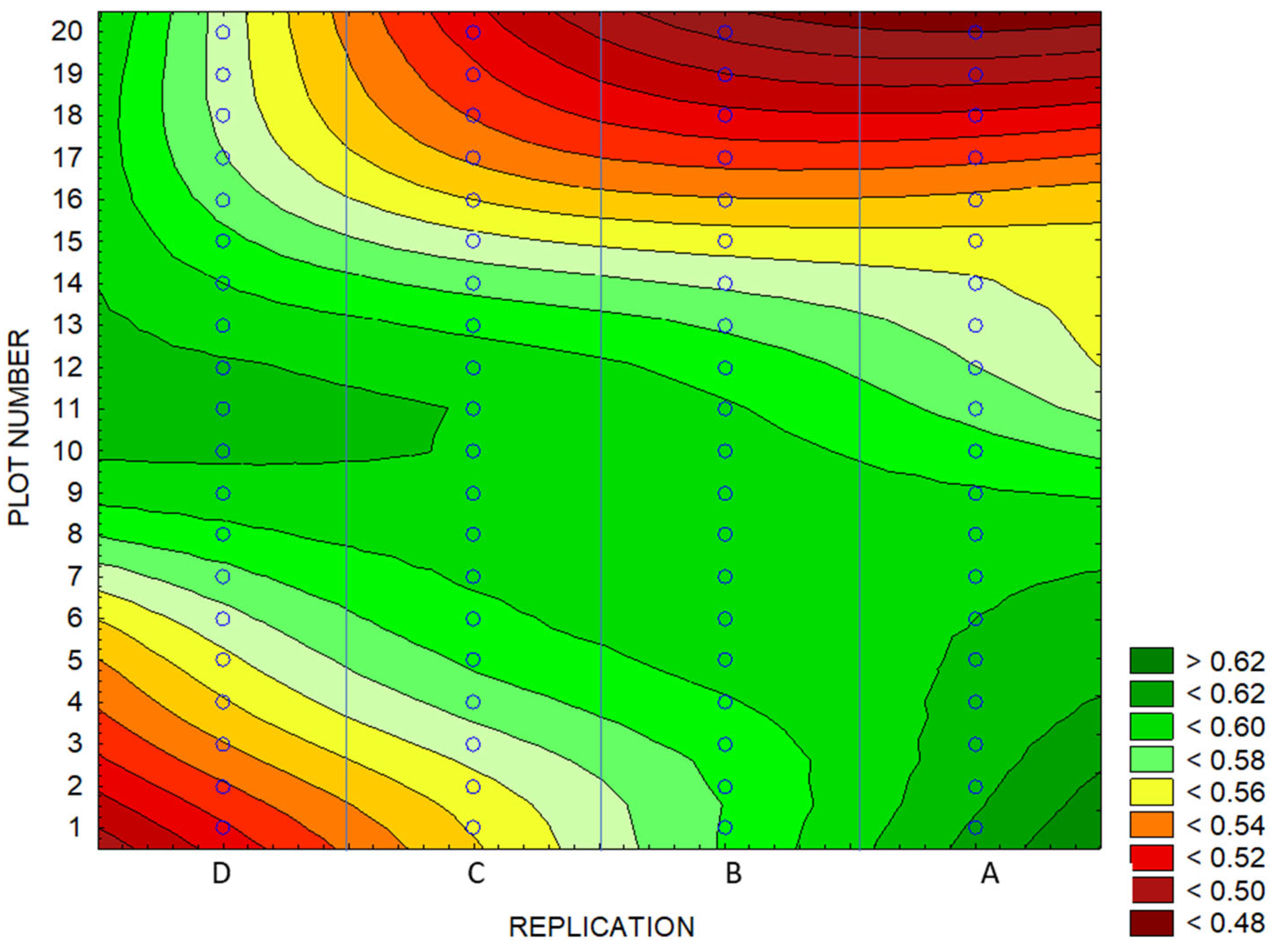
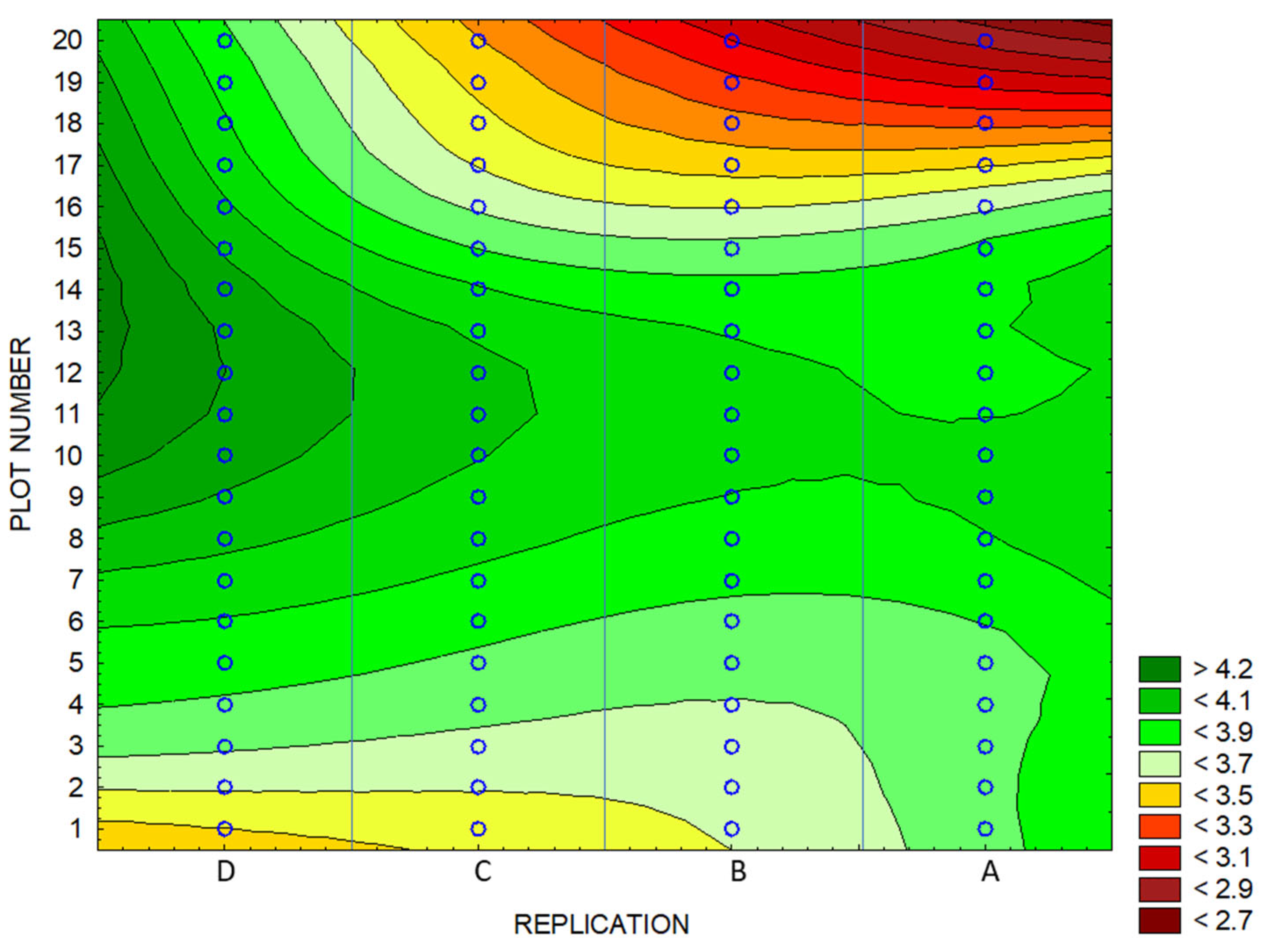
3.4. Identification of Anomalies in the Flowering Growth Condition Based on Vegetation Indices

Values of all three VI and yields on the experimental plots indicate that the values of studied parameters were deep below the overall average of experimental growth (3.77 t/ha) at the south-eastern edge (upper right corner) and north-western edge (lower left corner) of the experimental site. As to yield, the plots concerned were particularly 12A, 17, 18, 19, and 20 in the replications A and B; plots 15, 16, 17, 18, and 20 in the C replication; and plots 2B, 3B, 2C, 1D, and 2D (Figure 5b, Figure 6b and Figure 7b).

This is clearly shown on the contour maps constructed on the basis of NDVI, BNDVI, and NDYI values and yields from the individual plots (Figure 14, Figure 15, Figure 16 and Figure 17). The maps indicate that all studied VI reflect more or less identically spatial patterns of values almost identical to the distribution of crop yields.

Based on the data obtained, it is therefore possible to assume the existence of an edge effect, which occurred in the similar spatial patterns of vegetation indices and crop yield, and can be related to the variability of soil parameters in the field experiment. However, soil conditions in the studied area were not mapped in detail. Prevention to this growth variability, as it is demonstrated by the vegetation indices and partly also by the yields, was the randomized layout of experimental plots (Figure 2). Thus, a possible heterogeneity of the site is evenly distributed throughout all variants.

According to Mezera et al. [42], the spatial variability of the status of plants in fields reflects differences in soil properties, field topography, and management methods. If only the spectral soil images were analyzed, for example to determine the biological soil crust, then the site heterogeneity would affect negatively the result of such an experiment [43]. However, the goal of this study was not to find causes of growth status damage, identified on the basis of the low values of all three vegetation indices. We believe that on the contrary, the site heterogeneity can contribute to greater robustness of measured values as the correlation between the selected VI and OSR yield was positive and significant in spite of the detected site heterogeneity (Table 4, Figure 8, Figure 9 and Figure 10). In [34] for example, more than 229 various plots were analyzed for mapping the phenology of OSR flowering, taking into account neither the heterogeneity of used agricultural machines nor that of studied plots. By contrast, the heterogeneity that occurred within and between the individual plots (sites) contributed to greater robustness of measured values, and hence to the development of a strong model for predicting OSR yields, area, and production.

In order to verify the degree of influence of the edge effect on the values of VI and yields in the experiment, the individual plots were arbitrarily divided according to achieved yields into the area of low-yield plots (LOW-YIELD AREA) where the yields ranged within the interval of the lower quartile (Q25 = 3.51 t/ha) and the area of high-yield plots (HIGH-YIELD AREA) where the yields were higher than the lower quartile value. A complete overview is presented in Figure 18.

1.

LOW-YIELD AREA

YIELD ≤ Q25;

2.

HIGH-YIELD AREA

YIELD > Q25.

This division appeared to be more appropriate than that according to the average yield in the experiment as in a majority of cases the division according to Q₂₅ coincided to a considerable extent with the division of plots according to VI based on their Q₂₅. For each of these areas, average VI and yields were calculated (

Table 6. Comparison of the mean values of VI and yields for the experiment (WHOLE AREA) and GREEN AREA and RED AREA plots.

Experimental Areas	NDVI		BNDVI		NDYI		Yield
	Mean	Q25	Mean	Q25	Mean	Q25	Mean (t ha−1)	Q25
Whole Area	0.63	0.62	0.86	0.85	0.57	0.54	3.77	3.51
High-Yield Area	0.65		0.88		0.59		3.94
Low-Yield Area	0.61		0.84		0.52		3.24

).

The obtained values show that the mean yield of LOW-YIELD AREA (3.24 t/ha) was by 0.70 t/ha (18%) lower than the HIGH-YIELD AREA yield (3.94 t/ha), and the mean yield of the experiment WHOLE AREA (3.77 t/ha) was by 0.17 t/ha lower than the yield of HIGH-YIELD AREA (3.94 t/ha). Thus, the edge effect caused an average yield of the experiment reduced by 4.3%.

It can be concluded that the studied NDVI, BNDVI, and NDYI vegetation indices can be used for the identification of possible problems in the development of OSR growth at the stage of flowering. The high spatial resolution of the UAV surveying allows an accurate localization of the spatial unevenness of stands and hence targeted and efficient measures in line with the principles of precision agriculture. In their study, d’Adrimont et al. [34] demonstrated the usability of satellite surveying, namely detection of the date of OSR flowering date with an accuracy of 1–4 days using the NDYI vegetation index from the time series of multispectral satellite data Sentinel-1 and Sentinel-2. In addition to implementation for better accuracy of plant growth models, the information can also be used for timing the UAV monitoring of OSR at the time of flowering and for the following precise classification of flowering plants [26]. After all, UAV monitoring operability, versatility and risk-free piloting are the main factors of its popularity in agriculture [2].

As there may be a range of reasons causing undesirable development of crop growths, the solution of these problems is conditioned by further research.

4. Conclusions

In this study, a suitability of normalized differential vegetation index (NDVI), blue normalized differential vegetation index (BNDVI), and normalized differential yellowing index (NDYI) obtained using an unmanned aerial vehicle (UAV) at the stage of oil seed rape flowering was tested for the prediction of OSR yield and applicability of these vegetation indices for the identification of spatial variability of the status of plants in the stand based on the regression analysis. The correlation analysis performed to determine the degree of yield dependence on the values of NDVI, BNDVI, and NDYI indices showed that the seed yield exhibits a strong linear positive dependence on BNDVI (R = 0.98) and NDYI (R = 0.95). The correlation between the NDVI index and seed yield was weaker (R = 0.70). Coefficients of determination established on the basis of regression analysis were R² = 0.48 for NDVI, R² = 0.95 for BNDVI, and R² = 0.90 for NDYI. It is possible to state that the BNDVI index explains the variability of yield variable at 95% in this model and that yield prediction using BNDVI is the most accurate.

The performed analysis of indices NDVI, BNDVI, and NDYI demonstrated that these vegetation indices can be used to identify spatial variability of the status of OSR growth at the stage of flowering and hence also for targeted and efficient remedial measures in accordance with the principles of precision agriculture.

References

1. Cuaran, J.; Leon, J. Crop Monitoring using Unmanned Aerial Vehicles-A Review. Agric. Rev. 2021, 42, 121–132. [Google Scholar] [CrossRef]
2. Mukherjee, A.; Misra, S.; Raghuwanshi, N.S. A survey of unmanned aerial sensing solutions in precision agriculture. J. Netw. Comput. Appl. 2019, 148, 102461. [Google Scholar] [CrossRef]
3. Matese, A.; Toscano, P.; Gennaro, S.F.; Genesio, L.; Vaccari, F.P.; Primicerio, J.; Belli, C.; Zaldei, A.; Bianconi, R.; Gioli, B. Intercomparison of UAV, aircraft and satellite remote sensing platforms for precision viticulture. Remote Sens. 2015, 7, 2971–2990. [Google Scholar] [CrossRef] [Green Version]
4. Chapman, S.C.; Merz, T.; Chan, A.; Jackway, P.; Hrabar, S.; Dreccer, M.F.; Holland, E.; Zheng, B.; Ling, T.J.; Jimenez-Berni, J. Pheno-copter: A low-altitude, autonomous remote sensing robotic helicopter for high-throughput field-based phenotyping. Agron. J. 2014, 4, 279–301. [Google Scholar] [CrossRef] [Green Version]
5. Yang, C.; Hoffmann, W.C. Low-cost single-camera imaging system for aerial applicators. J. Appl. Remote Sens. 2015, 9, 096064. [Google Scholar] [CrossRef] [Green Version]
6. Gebbers, R.; Adamchuk, V.I. Precision Agriculture and Food Security. Science 2010, 327, 828–831. [Google Scholar] [CrossRef] [PubMed]
7. Bendig, J.; Bolten, A.; Bennertz, S.; Broscheit, J.; Eichfuss, S.; Bareth, G. Estimating Biomass of Barley using Crop Surface Models (CSMs) Derived from UAV-Based RGB Imaging. Remote Sens. 2014, 6, 10395–10412. [Google Scholar] [CrossRef] [Green Version]
8. López-Granados, F. Weed detection for site-specific weed management: Mapping and real-time approaches: Weed detection for site-specific weed management. Weed Res. 2011, 51, 1–11. [Google Scholar] [CrossRef] [Green Version]
9. Shi, Y.; Thomasson, J.A.; Murray, S.C.; Pugh, N.A.; Rooney, W.L.; Shafian, S.; Rajan, N.; Rouze, G.; Morgan, C.L.; Neely, H.L.; et al. Unmanned Aerial Vehicles for High-Throughput Phenotyping and Agronomic Research. PLoS ONE 2016, 11, e0159781. [Google Scholar] [CrossRef] [Green Version]
10. Vega, F.A.; Ramírez, F.C.; Saiz, M.P.; Rosúa, F.O. Multi- temporal imaging using an unmanned aerial vehicle for monitoring a sunflower crop. Biosyst. Eng. 2015, 132, 19–27. [Google Scholar] [CrossRef]
11. Sulik, J.J.; Long, D.S. Spectral considerations for modeling yield of canola. Remote Sens. Environ. 2016, 184, 161–174. [Google Scholar] [CrossRef] [Green Version]
12. Kumar, N.; Singh, S.K.; Obi Reddy, G.P.; Mishra, V.N.; Bajpai, R.K. Remote Sensing and Geographic Information System in Water Erosion Assessment. Agric. Rev. 2020, 41, 116–123. [Google Scholar] [CrossRef]
13. Gonzalez-de-Soto, M.; Emmi, L.; Perez-Ruiz, M.; Aguera, J.; Gonzalez-de-Santos, P. Autonomous systems for precise spraying–Evaluation of a robotised patch sprayer. Biosyst. Eng. 2016, 146, 165–182. [Google Scholar] [CrossRef]
14. Huang, Y.; Hoffmann, C.W.; Lan, Y.; Wu, W.; Fritz, B.K. Development of a Spray System for an Unmanned Aerial Vehicle Platform. Appl. Eng. Agric. 2008, 25, 803–809. [Google Scholar] [CrossRef]
15. Zhang, X.; He, Y. Rapid estimation of seed yield using hyperspectral images of oilseed rape leaves. Ind. Crop. Prod. 2013, 42, 416–420. [Google Scholar] [CrossRef]
16. Zhang, T.; Vail, S.; Duddu, H.S.N.; Parkin, I.A.P.; Guo, X.; Johnson, E.N.; Shirtliffe, S.J. Phenotyping Flowering in Canola (Brassica napus L.) and Estimating Seed Yield Using an Unmanned Aerial Vehicle-Based Imagery. Front. Plant Sci. 2021, 12, 686332. [Google Scholar] [CrossRef]
17. Leach, J.E.; Milford, G.F.J.; Mullen, L.A.; Scott, T.; Stevenson, H.J. Accumulation of Dry Matter in Oilseed Rape. Asp. Appl. Biol. 1989, 23, 117–123. [Google Scholar]
18. Shukla, G.; Tiwari, P.; Dugesar, V.; Srivastava, P.K. Chapter 9-Estimation of evapotranspiration using surface energy balance system and satellite datasets. In Agricultural Water Management, 1st ed.; Srivastava, P.K., Gupta, M., Tsakiris, G., Quinn, N.W., Eds.; Academic Press: Cambridge, MA, USA, 2021; pp. 157–183. [Google Scholar]
19. Becker-Reshef, I.; Vermote, E.; Lindeman, M.; Justice, C. A generalized regression-based model for forecasting winter wheat yields in Kansas and Ukraine using MODIS data. Remote Sens. Environ. 2010, 114, 1312–1323. [Google Scholar] [CrossRef]
20. Hancock, D.W.; Dougherty, C.T. Relationships between Blue- and Red-based Vegetation Indices and Leaf Area and Yield of Alfalfa. Crop Sci. 2007, 47, 2547. [Google Scholar] [CrossRef]
21. Sulik, J.J.; Long, D.S. Spectral indices for yellow canola flowers. Int. J. Remote Sens. 2015, 36, 2751–2765. [Google Scholar] [CrossRef]
22. Yates, D.J.; Steven, M.D. Reflexion and absorption of solar radiation by flowering canopies of oil-seed rape (Brassica napus L.). J. Agric. Sci. 1987, 109, 495–502. [Google Scholar] [CrossRef]
23. Shen, M.; Chen, J.; Zhu, X.; Tang, Y. Yellow flowers can decrease NDVI and EVI values: Evidence from a field experiment in an alpine meadow. Can. J. Remote Sens. 2009, 35, 99–106. [Google Scholar] [CrossRef]
24. Wan, L.; Cen, H.; Zhu, J.; Zhang, J.; Zhu, Y.; Sun, D.; Du, X.; Zhai, L.; Weng, H.; Li, Y.; et al. Grain yield prediction of rice using multi-temporal UAV-based RGB and multispectral images and model transfer—A case study of small farmlands in the South of China. Agric. For. Meteorol. 2020, 291, 108096. [Google Scholar] [CrossRef]
25. Domínquez, J.A.; Kumhálová, J.; Novák, P. Winter oilseed rape and winter wheat growth prediction sensing remote sensing methods. Plant. Soil. Environ. 2015, 65, 410–416. [Google Scholar]
26. Wan, L.; Li, Y.; Cen, H.; Zhu, J.; Yin, W.; Wu, W.; Zhu, H.; Sun, D.; Zhou, W.; He, Y. Combining UAV-Based Vegetation Indices and Image Classification to Estimate Flower Number in Oilseed Rape. Remote Sens. 2018, 10, 1484. [Google Scholar] [CrossRef] [Green Version]
27. Peng, Y.; Zhu, T.; Li, Y.; Dai, C.; Fang, S.; Gong, Y.; Wu, X.; Zhu, R.; Liu, K. Remote prediction of yield based on LAI estimation in oilseed rape under different planting methods and nitrogen fertilizer applications. Agric. For. Meteorol. 2019, 271, 116–125. [Google Scholar] [CrossRef]
28. FAO; IUSS. World Reference Base-Version 2015; 106; FAO: Rome, Italy, 2019; 197p, ISBN 978-92-5-131246-9. [Google Scholar]
29. Meier, U. Growth Stages of Mono-and Dicotyledonous Plants; Federal Biological Research Centre for Agriculture and Forestry: Bonn, Germany, 2001. [Google Scholar]
30. Rouse, J.W.; Haas, R.H.; Schell, J.A.; Deering, D.W. Monitoring vegetation systems in the Great Plains with ERTS. In Proceedings of the Third Earth Resources Technology Satellite-1 Symposium, Washington, DC, USA, 10–14 December 1973. Goddard Space Flight Center, NASA SP-351. Science and Technical Information Office, NASA: Washington, DC, USA, 1974. pp. 309–317.
31. Janoušek, J.; Jambor, V.; Marcoň, P.; Dohnal, P.; Synková, H.; Fiala, P. Using UAV-Based Photogrammetry to Obtain Correlation between the Vegetation Indices and Chemical Analysis of Agricultural Crops. Remote Sens. 2021, 13, 1878. [Google Scholar] [CrossRef]
32. Tucker, C.J.; Holben, B.N.; Elgin, J.H., Jr.; McMurtrey, J.E. Relationship of spectral data to grain yield variation (within a winter wheat field). Photogramm. Eng. Remote Sens. 1980, 46, 657–666. [Google Scholar]
33. Hodge, K.; Akhter, F.; Bainard, L.; Smith, A. Using an Unmanned Aerial Vehicle with Multispectral with RGB Sensors to Analyze Canola Yield in the Canadian Prairies. In Proceedings of the 14th International Conference on Precision Agriculture, Montreal, QC, Canada, 24–27 June 2018. [Google Scholar]
34. d’Andrimont, R.; Taymans, M.; Lemoine, G.; Ceglar, A.; Yordanov, M.; van der Velde, M. Detecting flowering phenology in oil seed rape parcels with Sentinel-1 and -2 time series. Remote Sens. Environ. 2020, 239, 111660. [Google Scholar] [CrossRef]
35. Barbosa, H.A.; Huete, A.R.; Baethgen, W.E. A 20-year study of NDVI variability over the Northeast Region of Brazil. J. Arid. Environ. 2006, 67, 288–307. [Google Scholar] [CrossRef]
36. Xue, J.; Su, B. Significant remote sensing vegetation indices: A review of developments and applications. J. Sens. 2017, 2017, 1353691. [Google Scholar] [CrossRef] [Green Version]
37. Shen, M.; Chen, J.; Zhu, X.; Tang, Y.; Chen, X. Do flowers affect biomass estimate accuracy from NDVI and EVI? Int. J. Remote Sens. 2010, 31, 2139–2149. [Google Scholar] [CrossRef]
38. Behrens, T.; Müller, J.; Diepenbrock, W. Utilization of canopy reflectance to predict properties of oilseed rape (Brassica napus L.) and barley (Hordeum vulgare L.) during ontogenesis. Eur. J. Agron 2006, 25, 345–355. [Google Scholar] [CrossRef]
39. Piekarczyk, J. Winter Oilseed-Rape Yield Estimates from Hyperspectral Radiometer Measurements. Quaest. Geogr. 2011, 30, 77–84. [Google Scholar] [CrossRef] [Green Version]
40. Migdall, S.; Ohl, N.; Bach, H. Parameterisation of the Land Surface Reflectance Model SLC for Winter Rape Using Spaceborne Hyperspectral CHRIS Data. ESA SP-683. In Proceedings of the Hyperspectral Workshop, Frascati, Italy, 17–19 March 2010. [Google Scholar]
41. Fan, H.; Liu, S.; Li, J.; Li, L.; Dang, L.; Ren, T.; Lu, J. Early prediction of the seed yield in winter oilseed rape based on the near-infrared reflectance of vegetation (NIRv). Comput. Electron. Agric. 2021, 186, 106166. [Google Scholar] [CrossRef]
42. Mezera, J.; Lukas, V.; Horniaček, I.; Smutný, V.; Elbl, J. Comparison of Proximal and Remote Sensing for the Diagnosis of Crop Status in Site-Specific Crop Management. Sensors 2022, 22, 19. [Google Scholar] [CrossRef]
43. Fischer, T.; Veste, M.; Eisele, A.; Bens, O.; Spyra, W.; Hüttl, R.F. Small scale spatial heterogeneity of Normalized Difference Vegetation Indices (NDVIs) and hot spots of photosynthesis in biological soil crusts. Flora Morphol. Distrib. Funct. Ecol. Plants 2012, 207, 159–167. [Google Scholar] [CrossRef]
Figure 1. Localization of the Troubsko experimental field station in CZE (Czech Republic) and European Union.
Remotesensing 14 04953 g001
Figure 2. Randomization of 20 experimental variants in four replications.
Remotesensing 14 04953 g002
Figure 3. The six-rotor UAV DJI Matrice M600 with Micasense Altum camera on the ground with calibration panel (left) and during the flight (right).
Remotesensing 14 04953 g003
Figure 4. (a) Orthomosaic image of field trial with OSR acquired by UAV on 1 May 2020 in RGB (a) and red color negative (b) band combination. Both images show the crop status at flowering stage and the intensity of flowers within the monitored area.
Remotesensing 14 04953 g004
Figure 5. Orthomosaic of NDVI values from the multispectral UAV survey from 1 May 2020 (a) and average NDVI values calculated for individual plots of the field trial (b).
Remotesensing 14 04953 g005
Figure 6. Orthomosaic of BNDVI values from the multispectral UAV survey from 1 May 2020 (a) and average BNDVI values calculated for individual plots of the field trial (b).
Remotesensing 14 04953 g006
Figure 7. Orthomosaic of NDYI values from the multispectral UAV survey from 1 May 2020 (a) and average NDYI values calculated for individual plots of the field trial (b).
Remotesensing 14 04953 g007
Figure 8. Graph of the variance of YIELD variable in relation to the measured NDVI values (N = 80). Source data (red squares) show the yields of each plot (Y-axis) divided into 11 groups according to NDVI measured on each plot, ranging from 0.57 to 0.67 (11 values; X-axis). The parcels in each of the 11 groups have the same NDVI value.
Remotesensing 14 04953 g008
Figure 9. Graph of the variance of YIELD variable in relation to the measured BNDVI values (N = 80). Source data (red squares) show the yields of each plot (Y-axis) divided into 9 groups according to BNDVI measured on each plot, ranging from 0.81 to 0.89 (9 values; X-axis). The parcels in each of the 9 groups have the same BNDVI value.
Remotesensing 14 04953 g009
Figure 10. Graph of the variance of YIELD variable in relation to the measured NDYI values (N = 80). Source data (red squares) show the yields of each plot (Y-axis) divided into 17 groups according to NDYI measured on each plot, ranging from 0.47 to 0.63 (17 values; X-;axis). The parcels in each of the 17 groups have the same NDYI value.
Remotesensing 14 04953 g010
Figure 11. Graph of linear dependence of yield on NDVI. Model shows yields observed and yields predicted based on the regression analysis of NDVI and yields achieved.
Remotesensing 14 04953 g011
Figure 12. Graph of linear dependence of yield on BNDVI. Model shows yields observed and yields predicted based on the regression analysis of NDVI and yields achieved.
Remotesensing 14 04953 g012
Figure 13. Graph of linear dependence of yield on NDYI. Model shows yields observed and yields predicted based on the regression analysis of NDYI and yields achieved.
Remotesensing 14 04953 g013
Figure 14. Contour map of NDVI. Blue circles illustrate plot centers.
Remotesensing 14 04953 g014
Figure 15. Contour map of BNDVI. Blue circles illustrate plot centers.
Remotesensing 14 04953 g015
Figure 16. Contour map of NDYI. Blue circles illustrate plot centers.
Remotesensing 14 04953 g016
Figure 17. Contour map of yields. Blue circles illustrate plot centers.
Remotesensing 14 04953 g017
Figure 18. Division of plots according to the value of the lower quartile of yields (Q25 = 3.51 t/ha) to LOW-YIELD AREA (yield ≤ Q25; color-coded plots) and HIGH-YIELD AREA (yield > Q25).
Remotesensing 14 04953 g018