


Sugarcane Biomass Prediction with Multi-Mode Remote Sensing Data Using Deep Archetypal Analysis and Integrated Learning
 , ,
, ,
Abstract
1. Introduction
2. Materials and Methods
2.1. Data Source
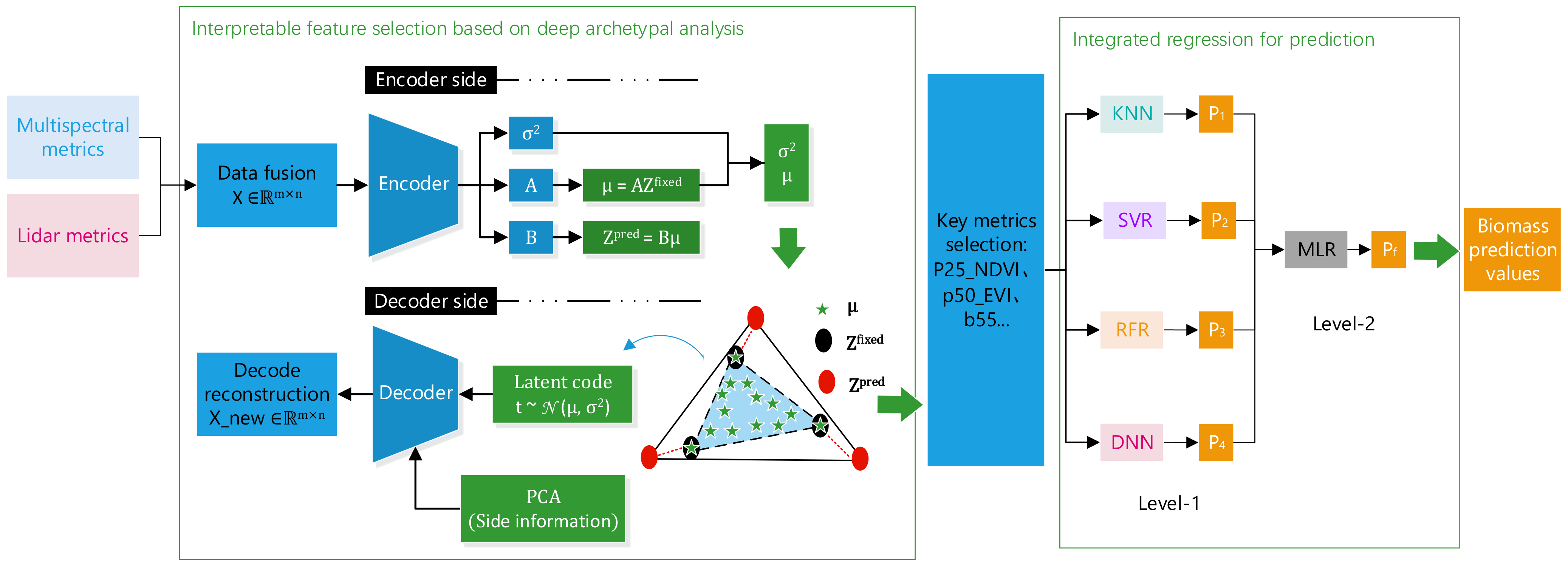
2.2. Method
2.2.1. Interpretable Feature Selection
2.2.2. Biomass Prediction with an Integrated Regression Model
2.3. Model Evaluation
3. Results
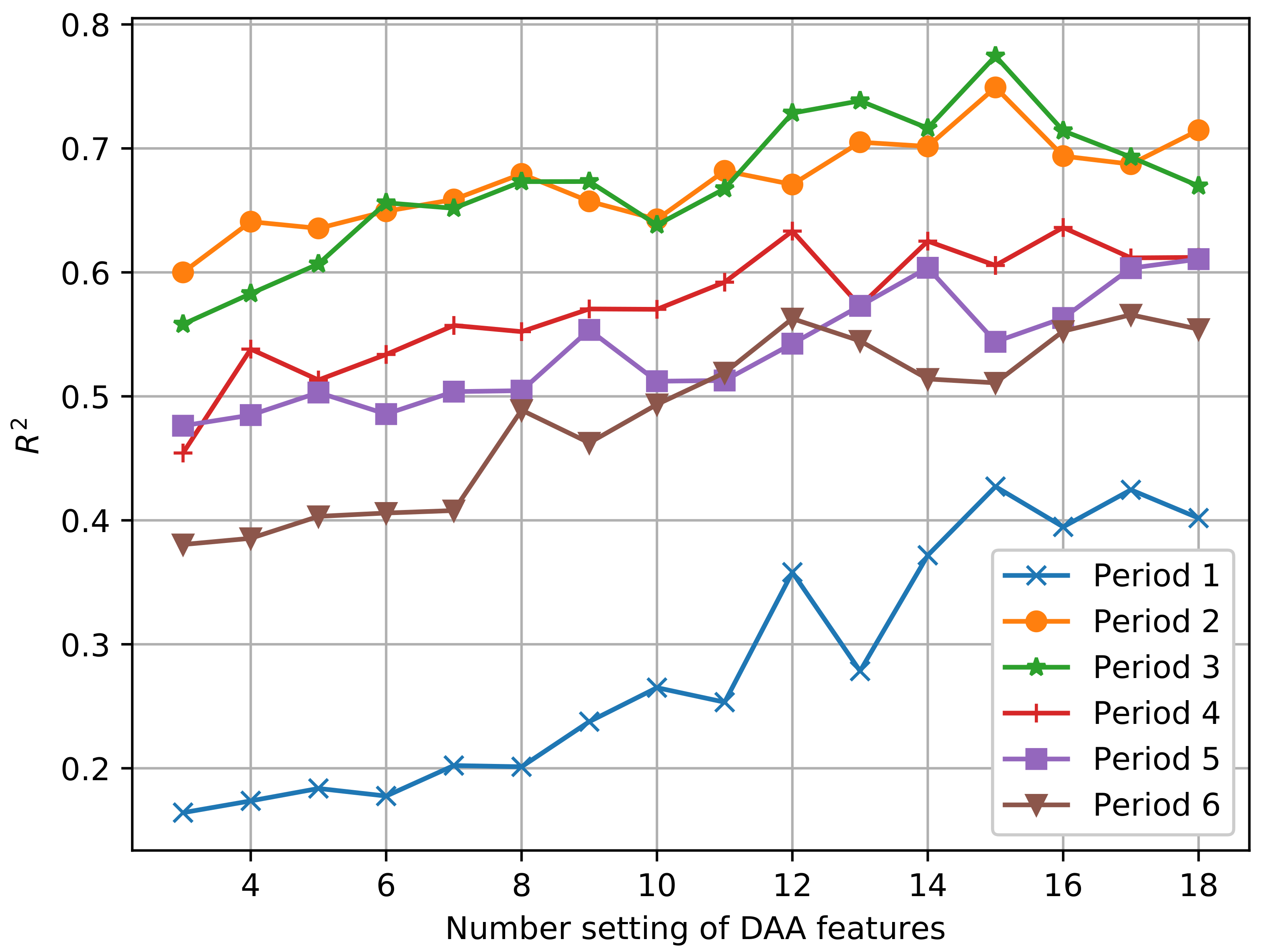
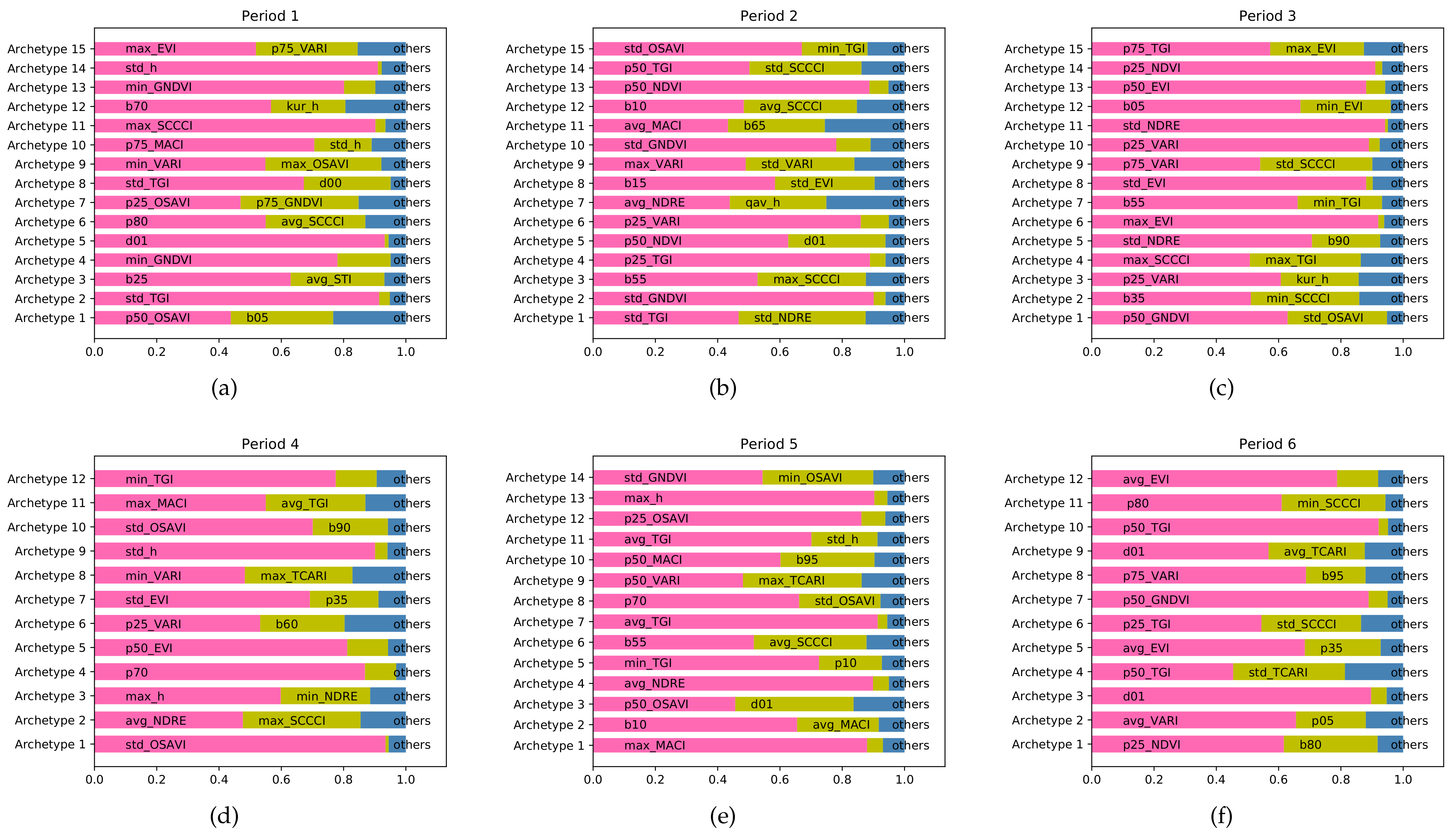
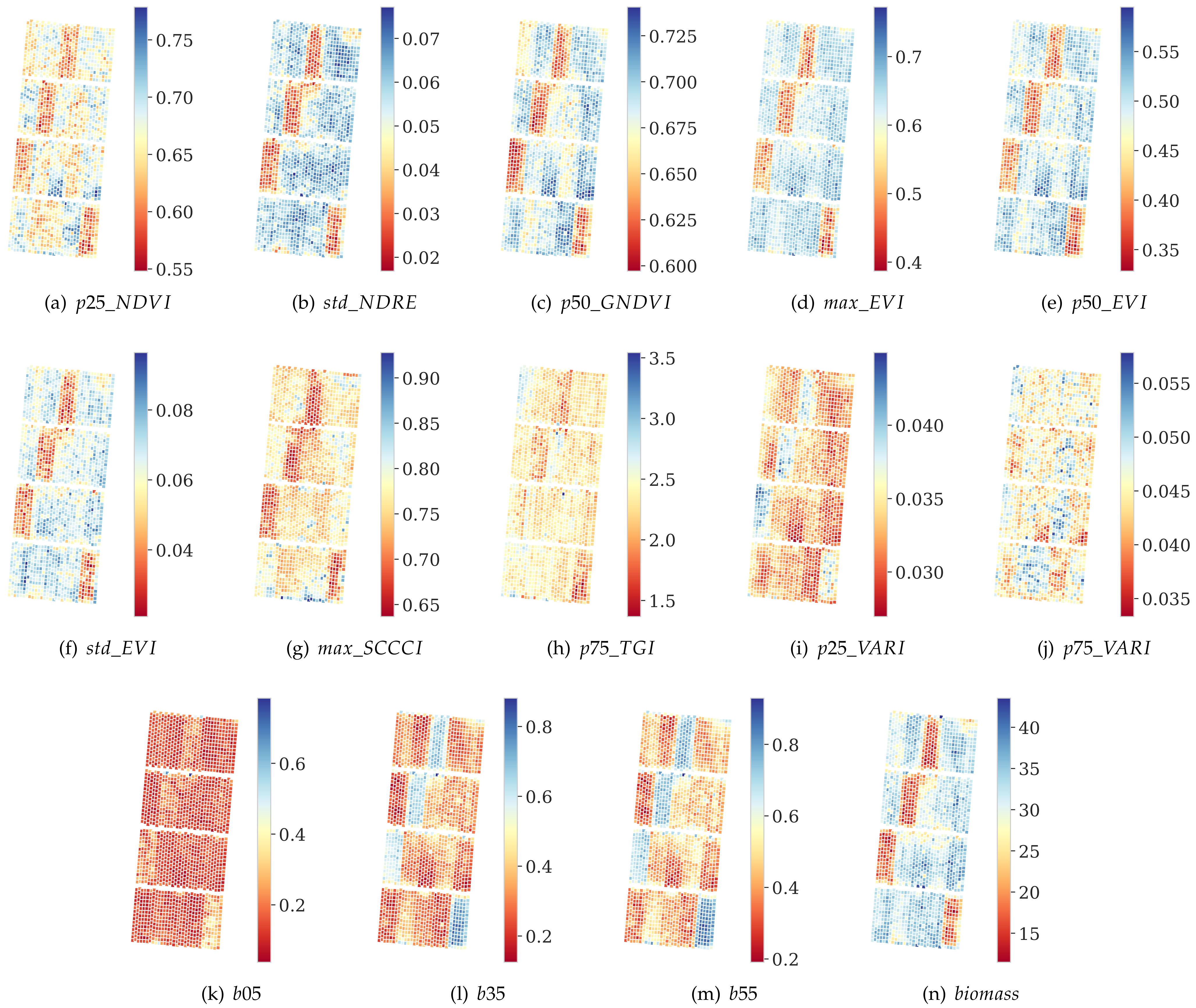
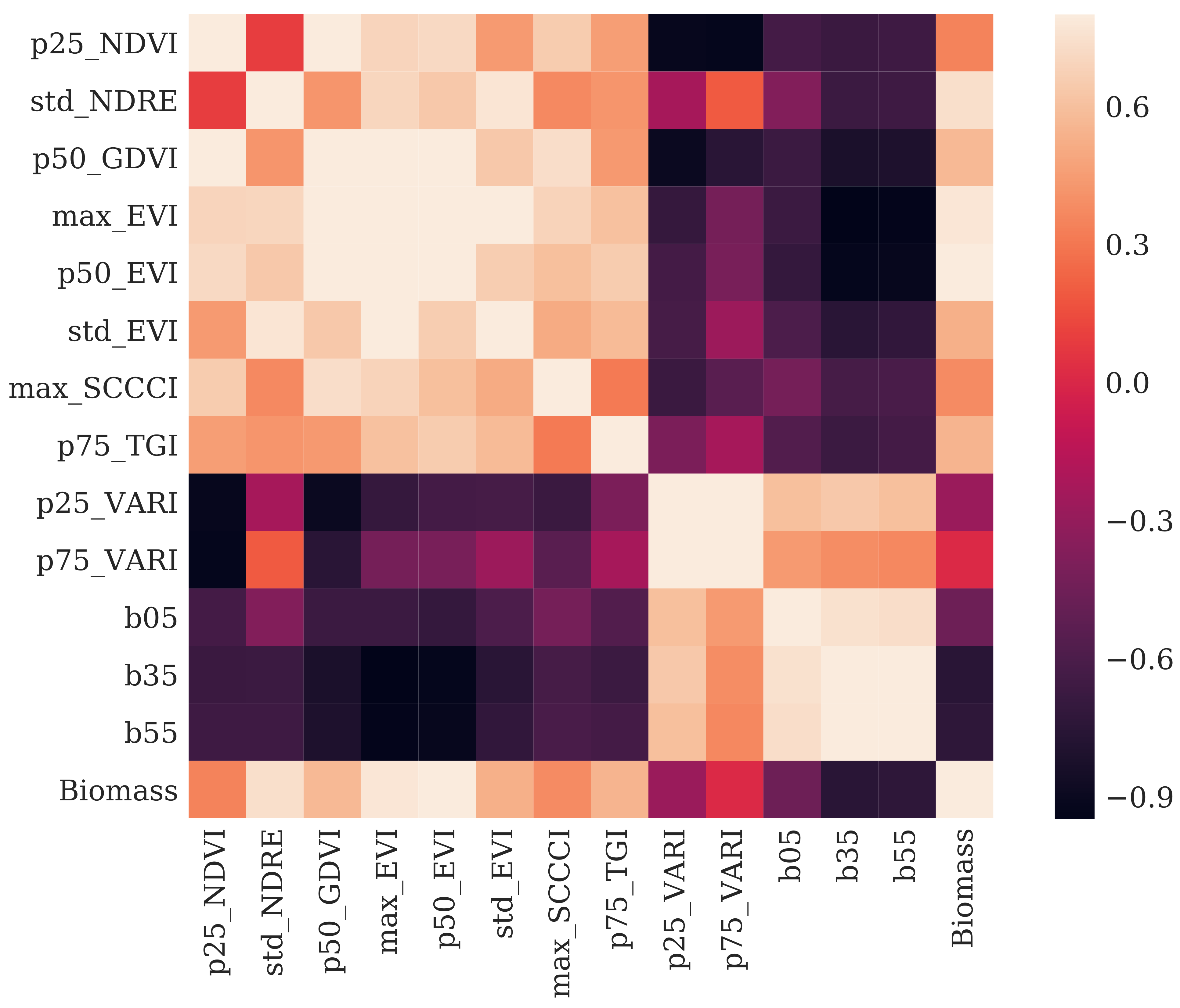
3.1. Multi-Source Data Feature Selection
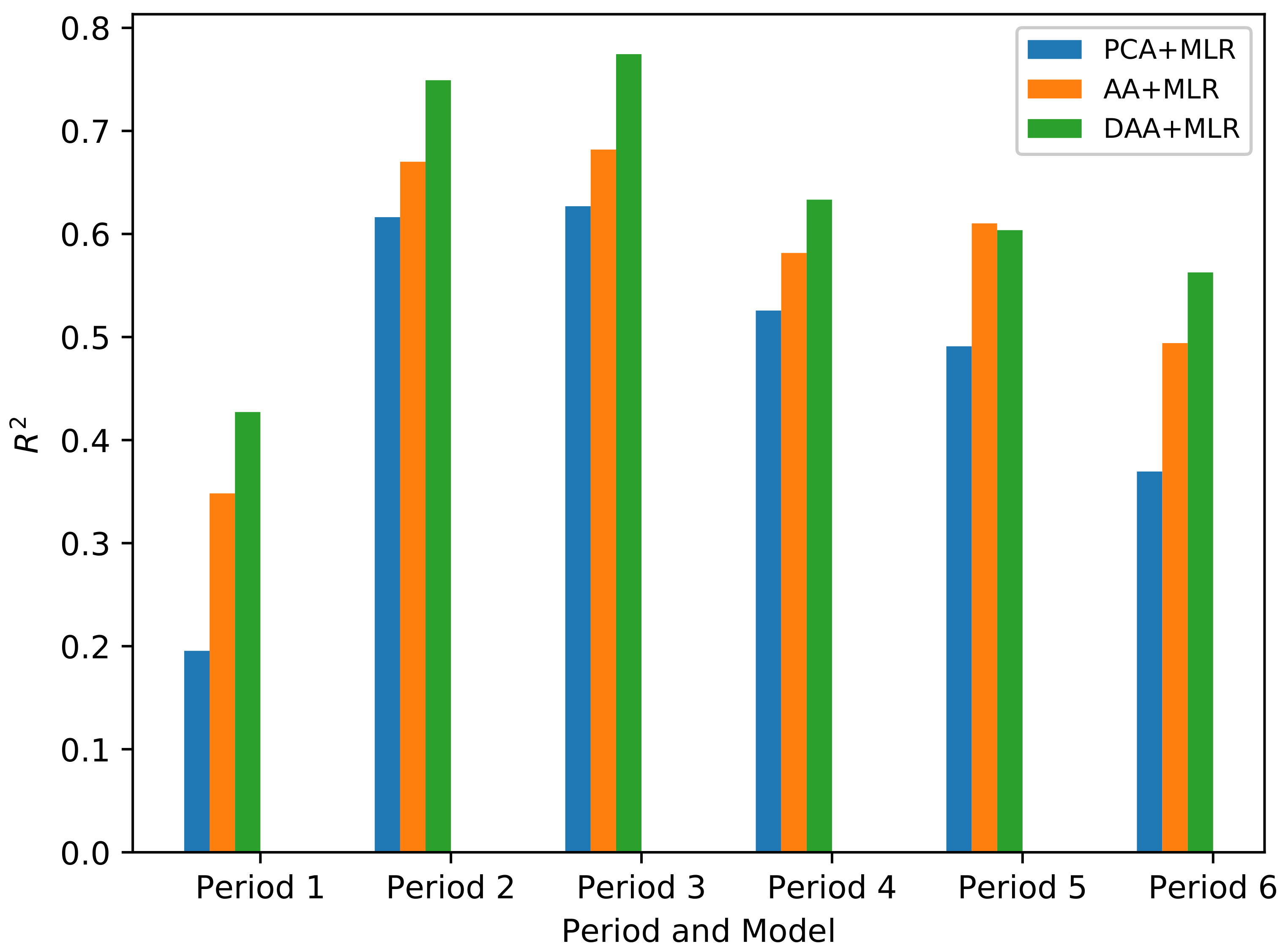
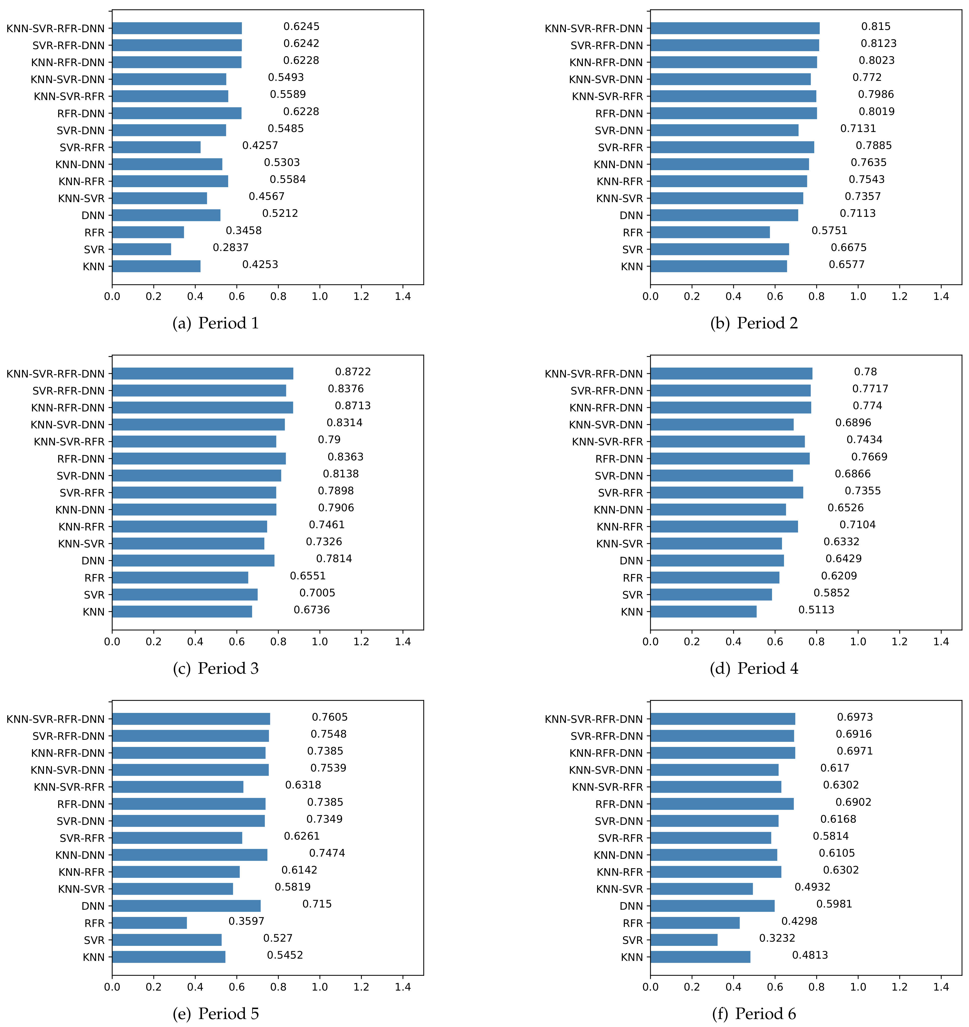
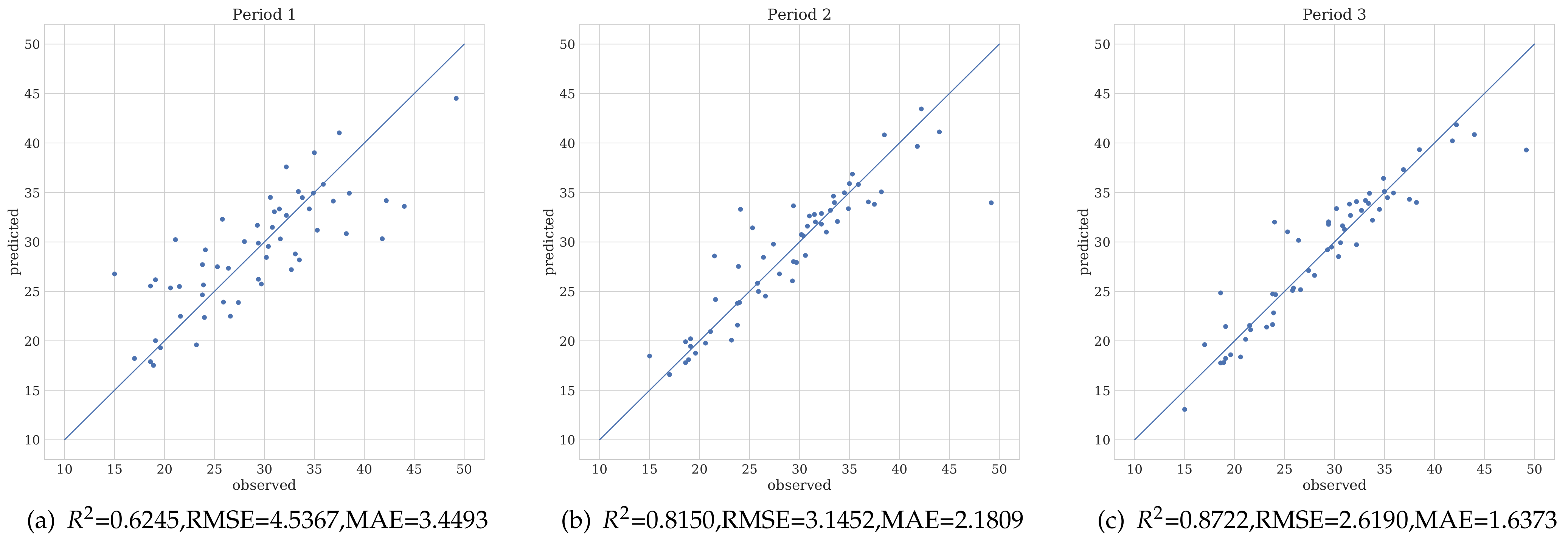
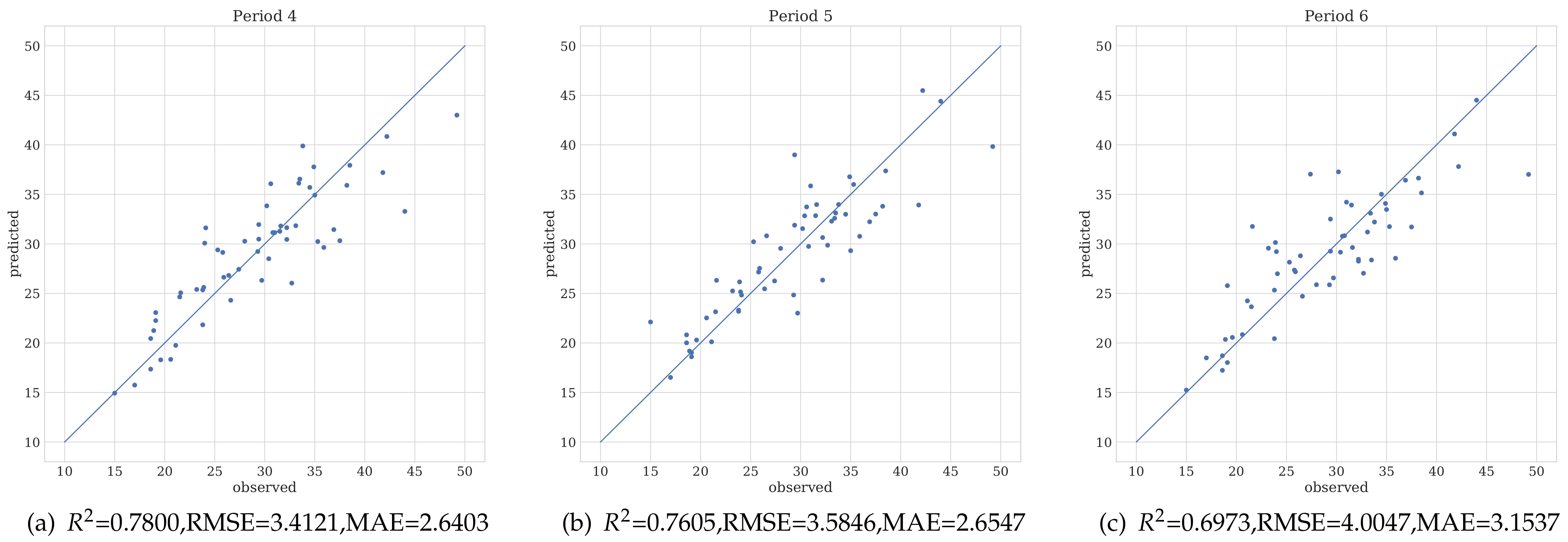
3.2. Biomass Prediction with Different Regression Models
4. Discussion
5. Conclusions
Author Contributions
Funding
Institutional Review Board Statement
Informed Consent Statement
Data Availability Statement
Conflicts of Interest
References
- Zhou, X.; Zheng, H.; Xu, X.; He, J.; Ge, X.; Yao, X.; Cheng, T.; Zhu, Y.; Cao, W.; Tian, Y. Predicting grain yield in rice using multi-temporal vegetation indices from UAV-based multispectral and digital imagery. ISPRS J. Photogramm. Remote Sens. 2017, 130, 246–255. [Google Scholar] [CrossRef]
- Yu, N.; Li, L.; Schmitz, N.; Tian, L.F.; Greenberg, J.A.; Diers, B.W. Development of methods to improve soybean yield estimation and predict plant maturity with an unmanned aerial vehicle based platform. Remote Sens. Environ. 2016, 187, 91–101. [Google Scholar] [CrossRef]
- Panda, S.S.; Ames, D.P.; Panigrahi, S. Application of vegetation indices for agricultural crop yield prediction using neural network techniques. Remote Sens. 2010, 2, 673–696. [Google Scholar] [CrossRef]
- Wang, L.; Tian, Y.; Yao, X.; Zhu, Y.; Cao, W. Predicting grain yield and protein content in wheat by fusing multi-sensor and multi-temporal remote-sensing images. Field Crop. Res. 2014, 164, 178–188. [Google Scholar] [CrossRef]
- Wan, L.; Cen, H.; Zhu, J.; Zhang, J.; Zhu, Y.; Sun, D.; Du, X.; Zhai, L.; Weng, H.; Li, Y.; et al. Grain yield prediction of rice using multi-temporal UAV-based RGB and multispectral images and model transfer—A case study of small farmlands in the South of China. Agric. For. Meteorol. 2020, 291, 108096. [Google Scholar] [CrossRef]
- Tucker, C.J. Red and photographic infrared linear combinations for monitoring vegetation. Remote Sens. Environ. 1979, 8, 127–150. [Google Scholar] [CrossRef]
- Sulik, J.J.; Long, D.S. Spectral considerations for modeling yield of canola. Remote Sens. Environ. 2016, 184, 161–174. [Google Scholar] [CrossRef]
- da Silva, E.E.; Baio, F.H.R.; Teodoro, L.P.R.; da Silva Junior, C.A.; Borges, R.S.; Teodoro, P.E. UAV-multispectral and vegetation indices in soybean grain yield prediction based on in situ observation. Remote Sens. Appl. Soc. Environ. 2020, 18, 100318. [Google Scholar] [CrossRef]
- Kouadio, L.; Newlands, N.K.; Davidson, A.; Zhang, Y.; Chipanshi, A. Assessing the performance of MODIS NDVI and EVI for seasonal crop yield forecasting at the ecodistrict scale. Remote Sens. 2014, 6, 10193–10214. [Google Scholar] [CrossRef]
- Maimaitijiang, M.; Ghulam, A.; Sidike, P.; Hartling, S.; Maimaitiyiming, M.; Peterson, K.; Shavers, E.; Fishman, J.; Peterson, J.; Kadam, S.; et al. Unmanned Aerial System (UAS)-based phenotyping of soybean using multi-sensor data fusion and extreme learning machine. ISPRS J. Photogramm. Remote Sens. 2017, 134, 43–58. [Google Scholar] [CrossRef]
- Christiansen, M.P.; Laursen, M.S.; Jørgensen, R.N.; Skovsen, S.; Gislum, R. Designing and testing a UAV mapping system for agricultural field surveying. Sensors 2017, 17, 2703. [Google Scholar] [CrossRef] [PubMed]
- Sofonia, J.; Shendryk, Y.; Phinn, S.; Roelfsema, C.; Kendoul, F.; Skocaj, D. Monitoring sugarcane growth response to varying nitrogen application rates: A comparison of UAV SLAM LiDAR and photogrammetry. Int. J. Appl. Earth Obs. Geoinf. 2019, 82, 101878. [Google Scholar] [CrossRef]
- Zhao, G.; Sanchez-Azofeifa, A.; Laakso, K.; Sun, C.; Fei, L. Hyperspectral and Full-Waveform LiDAR Improve Mapping of Tropical Dry Forest’s Successional Stages. Remote Sens. 2021, 13, 3830. [Google Scholar] [CrossRef]
- de Almeida, C.T.; Galvao, L.S.; Ometto, J.P.H.B.; Jacon, A.D.; de Souza Pereira, F.R.; Sato, L.Y.; Lopes, A.P.; de Alencastro Graça, P.M.L.; de Jesus Silva, C.V.; Ferreira-Ferreira, J.; et al. Combining LiDAR and hyperspectral data for aboveground biomass modeling in the Brazilian Amazon using different regression algorithms. Remote Sens. Environ. 2019, 232, 111323. [Google Scholar] [CrossRef]
- Cao, J.; Zhang, Z.; Tao, F.; Zhang, L.; Luo, Y.; Han, J.; Li, Z. Identifying the contributions of multi-source data for winter wheat yield prediction in China. Remote Sens. 2020, 12, 750. [Google Scholar] [CrossRef]
- Li, B.; Xu, X.; Zhang, L.; Han, J.; Bian, C.; Li, G.; Liu, J.; Jin, L. Above-ground biomass estimation and yield prediction in potato by using UAV-based RGB and hyperspectral imaging. ISPRS J. Photogramm. Remote Sens. 2020, 162, 161–172. [Google Scholar] [CrossRef]
- Zhang, N.; Chen, M.; Yang, F.; Yang, C.; Yang, P.; Gao, Y.; Shang, Y.; Peng, D. Forest Height Mapping Using Feature Selection and Machine Learning by Integrating Multi-Source Satellite Data in Baoding City, North China. Remote Sens. 2022, 14, 4434. [Google Scholar] [CrossRef]
- Shendryk, Y.; Sofonia, J.; Garrard, R.; Rist, Y.; Skocaj, D.; Thorburn, P. Fine-scale prediction of biomass and leaf nitrogen content in sugarcane using UAV LiDAR and multispectral imaging. Int. J. Appl. Earth Obs. Geoinf. 2020, 92, 102177. [Google Scholar] [CrossRef]
- Shi, Y.; Han, L.; Huang, W.; Chang, S.; Dong, Y.; Dancey, D.; Han, L. A Biologically Interpretable Two-Stage Deep Neural Network (BIT-DNN) for Vegetation Recognition From Hyperspectral Imagery. IEEE Trans. Geosci. Remote Sens. 2021, 60, 1–20. [Google Scholar] [CrossRef]
- Hong, D.; He, W.; Yokoya, N.; Yao, J.; Gao, L.; Zhang, L.; Chanussot, J.; Zhu, X. Interpretable hyperspectral artificial intelligence: When nonconvex modeling meets hyperspectral remote sensing. IEEE Geosci. Remote Sens. Mag. 2021, 9, 52–87. [Google Scholar] [CrossRef]
- Mørup, M.; Hansen, L.K. Archetypal analysis for machine learning and data mining. Neurocomputing 2012, 80, 54–63. [Google Scholar] [CrossRef]
- Cutler, A.; Breiman, L. Archetypal analysis. Technometrics 1994, 36, 338–347. [Google Scholar] [CrossRef]
- Seth, S.; Eugster, M.J. Probabilistic archetypal analysis. Mach. Learn. 2016, 102, 85–113. [Google Scholar] [CrossRef]
- Keller, S.M.; Samarin, M.; Arend Torres, F.; Wieser, M.; Roth, V. Learning extremal representations with deep archetypal analysis. Int. J. Comput. Vis. 2021, 129, 805–820. [Google Scholar] [CrossRef]
- Xu, J.X.; Ma, J.; Tang, Y.N.; Wu, W.X.; Shao, J.H.; Wu, W.B.; Wei, S.Y.; Liu, Y.F.; Wang, Y.C.; Guo, H.Q. Estimation of sugarcane yield using a machine learning approach based on uav-lidar data. Remote Sens. 2020, 12, 2823. [Google Scholar] [CrossRef]
- Stateras, D.; Kalivas, D. Assessment of olive tree canopy characteristics and yield forecast model using high resolution UAV imagery. Agriculture 2020, 10, 385. [Google Scholar] [CrossRef]
- Wang, Y.; Zhang, Z.; Feng, L.; Du, Q.; Runge, T. Combining multi-source data and machine learning approaches to predict winter wheat yield in the conterminous United States. Remote Sens. 2020, 12, 1232. [Google Scholar] [CrossRef]
- Breiman, L. Random forests. Mach. Learn. 2001, 45, 5–32. [Google Scholar] [CrossRef]
- Cortes, C.; Vapnik, V. Support-vector networks. Mach. Learn. 1995, 20, 273–297. [Google Scholar] [CrossRef]
- Aha, D.W.; Kibler, D.; Albert, M.K. Instance-based learning algorithms. Mach. Learn. 1991, 6, 37–66. [Google Scholar] [CrossRef]
- Zhang, Y.; Qin, Q.; Ren, H.; Sun, Y.; Li, M.; Zhang, T.; Ren, S. Optimal hyperspectral characteristics determination for winter wheat yield prediction. Remote Sens. 2018, 10, 2015. [Google Scholar] [CrossRef]
- Xu, C.; Ding, Y.; Zheng, X.; Wang, Y.; Zhang, R.; Zhang, H.; Dai, Z.; Xie, Q. A Comprehensive Comparison of Machine Learning and Feature Selection Methods for Maize Biomass Estimation Using Sentinel-1 SAR, Sentinel-2 Vegetation Indices, and Biophysical Variables. Remote Sens. 2022, 14, 4083. [Google Scholar] [CrossRef]
- Han, J.; Zhang, Z.; Cao, J.; Luo, Y.; Zhang, L.; Li, Z.; Zhang, J. Prediction of winter wheat yield based on multi-source data and machine learning in China. Remote Sens. 2020, 12, 236. [Google Scholar] [CrossRef]
- Haykin, S. Neural Networks, a Comprehensive Foundation; Prentice-Hall Inc.: New Jersey, NJ, USA, 1999; Volume 7458, pp. 161–175. [Google Scholar]
- Kross, A.; Znoj, E.; Callegari, D.; Kaur, G.; Sunohara, M.; Lapen, D.R.; McNairn, H. Using artificial neural networks and remotely sensed data to evaluate the relative importance of variables for prediction of within-field corn and soybean yields. Remote Sens. 2020, 12, 2230. [Google Scholar] [CrossRef]
- Yang, Q.; Shi, L.; Han, J.; Zha, Y.; Zhu, P. Deep convolutional neural networks for rice grain yield estimation at the ripening stage using UAV-based remotely sensed images. Field Crop. Res. 2019, 235, 142–153. [Google Scholar] [CrossRef]
- Feng, L.; Zhang, Z.; Ma, Y.; Du, Q.; Williams, P.; Drewry, J.; Luck, B. Alfalfa yield prediction using UAV-based hyperspectral imagery and ensemble learning. Remote Sens. 2020, 12, 2028. [Google Scholar] [CrossRef]
- Zhang, Z.; Pasolli, E.; Crawford, M.M. An adaptive multiview active learning approach for spectral–spatial classification of hyperspectral images. IEEE Trans. Geosci. Remote Sens. 2019, 58, 2557–2570. [Google Scholar] [CrossRef]
- Fei, S.; Hassan, M.A.; He, Z.; Chen, Z.; Shu, M.; Wang, J.; Li, C.; Xiao, Y. Assessment of ensemble learning to predict wheat grain yield based on UAV-multispectral reflectance. Remote Sens. 2021, 13, 2338. [Google Scholar] [CrossRef]
- Wolpert, D.H. Stacked generalization. Neural Netw. 1992, 5, 241–259. [Google Scholar] [CrossRef]
- Healey, S.P.; Cohen, W.B.; Yang, Z.; Brewer, C.K.; Brooks, E.B.; Gorelick, N.; Hernandez, A.J.; Huang, C.; Hughes, M.J.; Kennedy, R.E.; et al. Mapping forest change using stacked generalization: An ensemble approach. Remote Sens. Environ. 2018, 204, 717–728. [Google Scholar] [CrossRef]
- Feng, L.; Li, Y.; Wang, Y.; Du, Q. Estimating hourly and continuous ground-level PM2. 5 concentrations using an ensemble learning algorithm: The ST-stacking model. Atmos. Environ. 2020, 223, 117242. [Google Scholar] [CrossRef]
- Cai, Y.; Guan, K.; Lobell, D.; Potgieter, A.B.; Wang, S.; Peng, J.; Xu, T.; Asseng, S.; Zhang, Y.; You, L.; et al. Integrating satellite and climate data to predict wheat yield in Australia using machine learning approaches. Agric. For. Meteorol. 2019, 274, 144–159. [Google Scholar] [CrossRef]
- Son, N.; Chen, C.; Chen, C.; Minh, V.; Trung, N. A comparative analysis of multitemporal MODIS EVI and NDVI data for large-scale rice yield estimation. Agric. For. Meteorol. 2014, 197, 52–64. [Google Scholar] [CrossRef]
- Hatfield, J. Remote sensing estimators of potential and actual crop yield. Remote Sens. Environ. 1983, 13, 301–311. [Google Scholar] [CrossRef]


| Period | Optimal Number of Archetypes Set | Features Obtained with Optimal Archetype Parameter Settings | |
|---|---|---|---|
| Period 1 | 15 | 0.4272 | |
| Period 2 | 15 | 0.7492 | |
| Period 3 | 15 | 0.7745 | |
| Period 4 | 12 | 0.6333 | |
| Period 5 | 14 | 0.6037 | |
| Period 6 | 12 | 0.5627 |
| Model | Period 1 | Period 2 | Period 3 | Period 4 | Period 5 | Period 6 |
|---|---|---|---|---|---|---|
| KNN | 0.1398 | 0.2525 | 0.0972 | −0.2492 | −0.5308 | −0.0431 |
| SVR | −0.0553 | −0.3792 | −1.3946 | 0.2296 | 0.2276 | −0.2325 |
| RFR | 0.5010 | 0.3148 | 0.3660 | 0.4844 | 0.1298 | 0.3683 |
| DNN | 0.6330 | 0.8390 | 1.9695 | 0.6946 | 1.1441 | 0.8115 |
Publisher’s Note: MDPI stays neutral with regard to jurisdictional claims in published maps and institutional affiliations. |
© 2022 by the authors. Licensee MDPI, Basel, Switzerland. This article is an open access article distributed under the terms and conditions of the Creative Commons Attribution (CC BY) license (https://creativecommons.org/licenses/by/4.0/).
Share and Cite
Wang, Z.; Lu, Y.; Zhao, G.; Sun, C.; Zhang, F.; He, S. Sugarcane Biomass Prediction with Multi-Mode Remote Sensing Data Using Deep Archetypal Analysis and Integrated Learning. Remote Sens. 2022, 14, 4944. https://doi.org/10.3390/rs14194944
Wang Z, Lu Y, Zhao G, Sun C, Zhang F, He S. Sugarcane Biomass Prediction with Multi-Mode Remote Sensing Data Using Deep Archetypal Analysis and Integrated Learning. Remote Sensing. 2022; 14(19):4944. https://doi.org/10.3390/rs14194944
Chicago/Turabian StyleWang, Zhuowei, Yusheng Lu, Genping Zhao, Chuanliang Sun, Fuhua Zhang, and Su He. 2022. "Sugarcane Biomass Prediction with Multi-Mode Remote Sensing Data Using Deep Archetypal Analysis and Integrated Learning" Remote Sensing 14, no. 19: 4944. https://doi.org/10.3390/rs14194944
APA StyleWang, Z., Lu, Y., Zhao, G., Sun, C., Zhang, F., & He, S. (2022). Sugarcane Biomass Prediction with Multi-Mode Remote Sensing Data Using Deep Archetypal Analysis and Integrated Learning. Remote Sensing, 14(19), 4944. https://doi.org/10.3390/rs14194944