Patterns, Dynamics, and Drivers of Soil Available Nitrogen and Phosphorus in Alpine Grasslands across the QingZang Plateau

Abstract

Soil available nutrient contents are critical for regulating ecosystem structure and function; therefore, exploring patterns, dynamics, and drivers of soil available nutrient contents is helpful for understanding the geochemical cycle at the regional scale. However, learning the patterns and dynamics of soil available nutrients across a regional scale is quite limited, especially the soil available nitrogen (SAN) and soil available phosphorus (SAP) in alpine grasslands. In this study, we used machine learning (Random Forest) to map the SAN and SAP at a soil depth of 0–30 cm in alpine grasslands across the QingZang Plateau (QZP) in 2015. Our results showed that the current (2015) contents of the SAN and SAP in alpine grasslands on the QZP were 139.96 mg kg⁻¹ and 2.63 mg kg⁻¹, respectively. Compared to the 1980s, the SAN significantly increased by 18.12 mg kg⁻¹ (14.83%, p < 0.05) and the SAP decreased by 1.71 mg kg⁻¹ (39.40%, p < 0.05). The SAN and SAP contents of alpine meadows were higher than those of alpine steppes. The increases in SAN were not significantly (p > 0.05) different between those two grassland types, while the decrease in SAP was significantly (p < 0.05) higher in alpine meadows than in alpine grasslands. Combined with redundancy analysis, we quantified the impact of environmental drivers, and 80% of the spatial variation in SAN and SAP could be explained by environmental factors. Our findings also highlighted that in the context of global change, the increase in SAP and decrease in SAP might lead to weakening of nitrogen limitation and intensification of phosphorus limitation, especially in alpine meadows. In general, this study expanded the knowledge about the patterns and dynamics of SAN and SAP, and deepened the understanding of the driving mechanisms, which provided a basis for sustainable management of grasslands and optimization of ecological security barrier functions on the QZP.

1. Introduction

Soil nutrient availability performs essential effects on regulating plant–soil feedbacks [1] and terrestrial ecosystem nutrient cycling [2]. Nitrogen (N) and phosphorus (P) are the primary soil nutrients that limit vegetation productivity [3,4,5], and their availability and dynamics alter ecosystem structure and functions by affecting species diversity [2,6], thus regulating the terrestrial ecosystem carbon cycle [7,8]. N enters the ecosystem mainly through nitrogen fixation, while P relies mainly on weathering of native minerals [9]. Soil available nitrogen (SAN) and soil available phosphorus (SAP) are the nutrients that can be directly used by vegetation from the soil. Importantly, soil nutrient cycling processes are significantly influenced by biotic and abiotic environmental factors and controlled by different mechanisms [10], whereby variations in environmental factors can potentially affect the patterns and dynamics of SAN and SAP [11]. Furthermore, numerous studies have shown that N limitation and P limitation are prevalent throughout terrestrial ecosystems [12,13,14,15]. It is noted that although the dynamics and mechanisms of SAN and SAP have been explored via the experiment sites or transects, the patterns and dynamics of SAN and SAP at the regional scale are still unclear.

Assessing soil available nutrient dynamics at large scales is critical for understanding regional nutrient cycling. The high spatial and temporal variability of environmental factors and the complex interactions among them result in the high spatiotemporal heterogeneity of the soil available nutrients [16]. It is difficult to accurately obtain the patterns and dynamics of SAN and SAP on a large scale. Traditional models such as spatial interpolation, area-weighted averaging based on spatial constraints of soil taxonomic units, and empirical functions are widely used to estimate the soil properties of regions [17,18,19]. However, these methods suffer from poor spatial representation and low resolution [20,21]. More recent research adopted advanced machine learning [22,23,24,25] (e.g., Random Forest) methods to simulate the spatiotemporal patterns of soil nutrients with substantial assessment results. For instance, the International Soil Reference Information Center (ISRIC) mapped the spatial distribution of global soil properties based on a machine learning approach (SoilGrids250) [26]. Furthermore, the Random Forest model was introduced to investigate the dynamics and driving forces of soil organic carbon in China [27]. Apparently, machine learning models and the validation processes could help us to improve our understanding of the spatial heterogeneity of soil nutrients [28], and the modeled results could clarify the controls of soil nutrients [29]. To the best of our knowledge, only a few studies examined the variations of SAN and SAP via a machine learning method at a large scale, especially across the QingZang Plateau (QZP).

According to the previous studies, patterns and dynamics of SAN and SAP are regulated by various drivers, including climate, geography, soil parent material, microbes, vegetation dynamics [30,31,32,33], and human activities [34]. Biotic and abiotic environments have been altered due to climate change, which has profound effects on biogeochemical processes [35]. Numerous studies have demonstrated that global-warming-caused perennial permafrost degradation may release soil nutrients (including SAN and SAP) that are beneficial to plant growth [36,37]. Specifically, the rising temperature facilitates the decomposition of soil organic matter and promotes the accumulation and cycling of soil available nutrients [38]. However, the increased temperature possibly reduces the availability of soil nutrients [39], since the hydrothermal conditions trigger soil nutrient imbalance or cyclic decoupling by altering surface temperature, soil moisture content, and microbial activities [40,41], and thereby affect vegetation growth, community composition, and ecosystem functions [42,43]. Remarkably, the increased anthropogenic nitrogen emissions have enhanced the atmospheric nitrogen deposition in grassland areas of northern China in recent decades [44], with increasing rates varying between 5.2 and 18.7 kg N ha⁻¹ yr⁻¹ [45], and the elevated nitrogen deposition has been demonstrated to further affect the nitrogen status of ecosystems significantly [44]. The availability of soil phosphorus is controlled by long-term biogeochemical processes [46] and can be affected by environmental factors. For instance, temperature can directly perturb soil phosphorus adsorption and desorption [47], while precipitation can regulate soil phosphorus leaching [48]. In addition, processes such as erosion, dissolution, and landslides caused by topographic conditions can lead to nutrient accumulation or loss in different areas [16]. Consequently, recognizing the drivers of the variations of SAN and SAP at the large regional scale is crucial for understanding the underlying mechanism of soil nutrient cycling and the principles of terrestrial ecosystems.

The QZP is an important ecological security barrier in China, whose alpine ecosystems are more sensitive to global change than other regions [49]. Alpine grassland is the major ecosystem type on the QZP. Hence, clarifying the patterns and dynamics of SAN and SAP is crucial to promoting sustainable grassland management and optimizing the function of ecological security barriers. In summary, the purpose of this study is to investigate the patterns, dynamics, and drivers of SAN and SAP in alpine grasslands on the QZP. Firstly, we quantified the spatial patterns of SAN and SAP in 2015 using a Random Forest model by employing field sampling data. Then, the historical soil available nutrient data (1980s) were used to further quantify the changes in SAN and SAP to investigate their temporal dynamics. Last but not least, we calculated the explanatory rates of different environmental factors on the spatial patterns of SAN and SAP to explore the driving mechanisms involved.

2. Materials and Methods

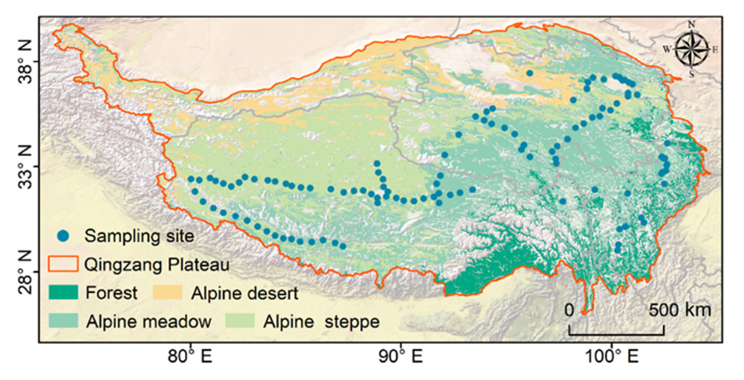
2.1. Study Area

The QingZang Plateau (QZP), located in the southwest of China (26°00′12″N to 39°46′50″N and 73°18′52″E to 104°46′59″E, Figure 1), is one of the highest (average altitude approximately 4000 m) and the most extensive (approximately 2.5 million km²) plateaus in the world [49,50]. Grassland, mainly consisting of alpine steppe and alpine meadow, is the major ecosystem type of the QZP ([51]). The QZP is known as “Asia’s Water Tower” and the “Amplifier of Global Climate Change” ([49]), and acts as an important ecological security barrier for China. The QZP is characterized by extreme climate and harsh environment [52,53], and there is an obvious gradient in temperature and precipitation under the influence of topographical and geographical conditions [54]. The mean annual precipitation is 486 mm, with precipitation mainly concentrated from June to September, and the mean annual temperature ranges from −6 °C to 3 °C [52]. Soil grades mainly consist of Gelisols, Inceptisols, Mollisols, Aridisols, and Entisols [55].

2.2. Data Collection

2.2.1. Soil Available Nitrogen and Phosphorus Samples

To quantitatively estimate SAN and SAP contents over the QZP, we sampled 115 alpine grassland sites (345 samples) along the transect on the QZP during the summer of 2015 (July and August) (Figure 1) [54]. The field sample sites were selected based on visual inspection, which were located on flat terrain, away from roads, and with low grazing intensity to reduce anthropogenic disturbances [56]. At each sample site (10 m × 10 m), three locations were randomly selected for soil sample collection, where the soil samples were collected at a depth of 0–30 cm using a soil auger. The latitude and longitude of each sample site were recorded by handheld GPS. In the laboratory, soil samples were air-dried and then sieved through 2 mm mesh, and the SAN and SAP were measured by the alkali-hydrolyzed reduction-diffusion method and the Olsen method [56,57], respectively. It is worth mentioning that 80% of the SAN and SAP random sample data were used as training data for the Random Forest (RF) model and the remaining 20% of data were testing data.

2.2.2. Environmental Factors

In total, 44 environmental raster datasets, including four categories, climate, geography, soil, and vegetation, were constructed for RF inversion and driver analysis. Detailed information and data sources for each indicator are described in the Supplementary Materials (Table S1). In particular, Slope and Aspect data were derived from DEM data in ArcGIS10.6, soil data were calculated as the average values of 0–30 cm on the Google Earth Engine (GEE) platform, and vegetation phenology data (SOS, LOS, EOS) were obtained using NDVI data in Matlab. Furthermore, these raster datasets were resampled to 30 s (~1 km at the equator) and the multi-year averages were calculated for refinement inversion of SAN and SAP contents.

The vegetation types (Figure 1) were divided according to the 1:1 million China vegetation map (Resource and Environment Data Cloud Platform, https://www.resdc.cn/data.aspx?DATAID=122, accessed on 1 September 2021). Additionally, the historical soil available nutrient data (1980s) used to calculate the SAN and SAP changes were obtained from the Land–Atmosphere Interaction Research Group of Sun Yat-sen University (http://globalchange.bnu.edu.cn/research/soil2, accessed on 20 November 2021), and the first three layers of data (0–30 cm) with the resolution of 30 s were used in this study.

2.3. SAN and SAP Estimation Based on Random Forest

2.3.1. Environmental Covariates Selection

We performed the multicollinearity analysis and independence detections on the 44 environmental covariates using variance inflation (VIF) and tolerance (TOL) to screen the indicators with VIF < 10 and TOL > 0.1 for training RF models [58,59]. Then, the selected environmental covariates were matched to the field sample points by latitude and longitude coordinates for training and testing of the RF models.

2.3.2. Random Forest Modeling

RF is an ensemble machine learning algorithm that operates by building a series of regression trees based on a sample dataset [16,60]. The RF model can enhance the accuracy of prediction and inversion by aggregating the results of multiple decision trees and showing better resistance to experimental noise interference [27]. Many previous studies have been conducted to apply RF for the prediction and inversion of regional-scale data [16,58,61]. Therefore, we applied the RF models to estimate the spatial pattern of SANs and SAPs across the QZP.

In our RF models, 80% of the sample and covariate datasets were used for training. We used a grid search to iteratively explore the optimal parameters of models (hyperparametric grid settings: number of subtrees (n_estimators: 1 to 100), the maximum growth depth of the tree (max_depth: 1 to 5), the minimum number of samples of leaves (min_samples_leaf: 1 to 30), and the maximum number of selected features (max_features: 1 to 15)). During the grid search, the performance of each model iteration was evaluated by randomized 10-fold cross-validation and out-of-bag estimation, and the optimal models were obtained by gradually improving the score of the models. Finally, we ran the optimal models 10 times based on the covariate dataset to obtain the means and standard deviations of the SAN and SAP in raster scale as the estimates and uncertainties of SAN and SAP. The RF models were run based on the “sklearn” package in Python [62].

2.3.3. Evaluation Model

To verify the accuracy of the inverse estimations of the RF models, we calculated the Pearson correlation coefficient (r), coefficient of determination (R-square), and the root mean squared error (RMSE) using the remaining 20% of the test data and model estimation data to quantify the bias of the RF models. The RMSE is calculated as follows:

$$\mathrm{RMSE}=\sqrt{\frac{{{\displaystyle \sum }}_{i=1}^n{\left(x_i-y_i\right)}^2}{n}}$$

(1)

where $n$ is the number of test data, $x_i$is the test data, and $y_i$is the model estimation data [59]. Importantly, we performed the normality test (α = 0.05) on the test data and the model estimation data using skewness and kurtosis.

In addition, the standard deviations of the 10-fold cross-validation were used as uncertainties to further validate the spatial predictive ability (robustness) of the models, reflecting the errors caused by random sampling [27].

2.4. Data Analysis

2.4.1. Spatiotemporal Analysis

After estimating and mapping the SAN and SAP (2015) by RF, we compared the results to the historical soil available nutrient data (1980s) to quantify the temporal variations in SAN and SAP on the QZP. Meanwhile, an exploratory spatial data analysis (ESDA) based on GIS technology was performed to reveal the spatial interactions of the results [63]. ESDA methods include global spatial autocorrelation (Global Moran’s Index) and local spatial autocorrelation (Getis-ord Gi* Index).

Quantifying SAN and SAP temporal dynamics. We quantified the temporal dynamics in SAN and SAP by the following equations:

$${\Delta SAN=SAN}_{estimated}-{ SAN}_{historical}$$

(2)

$${\Delta SAP=SAP}_{estimated}-{ SAP}_{historical}$$

(3)

where $\Delta SAN$ and $\Delta SAP$ are the temporal dynamics of SAN and SAP, ${SAN}_{estimated}$ and $SA{P}_{estimated}$ are the estimates from RF, and ${SAN}_{historical}$ and ${SAP}_{historical}$ are historical soil available nutrient data.

Global Moran’s Index. The Global Moran’s Index [64] was used to measure the extent of spatial correlation of the results across the QZP. The calculation method is as follows:

$$I=\frac{{{\displaystyle \sum }}_{i=1}^n{{\displaystyle \sum }}_{j=1}^n{w}_{ij}\left(x_i-\overline{x}\right)\left(x_j-\overline{x}\right)}{S^2\times {{\displaystyle \sum }}_{i=1}^n{{\displaystyle \sum }}_{j=1}^n{w}_{ij}},S^2=\frac{1}{n}{\displaystyle {{\displaystyle \sum }}_{i=1}^n}{\left(x_i-\overline{x}\right)}^2$$

(4)

where $n$ shows the total number of pixels; $x_i$and $x_j$ represent the values of pixel $i$ and pixel $j$; $\overline{x}$ denotes the average value of all pixels; $w_{ij}$ is the spatial weight matrix constructed by Queen and Rook; $S^2$ represents the variance of all pixels. The value of Global Moran’s I ranged from −1 to 1. I > 0 means a positive correlation, with high or low values aggregated, I < 0 means a negative correlation, with high and low values adjacent to each other, and I = 0 represents that the data are randomly distributed and there was no correlation. In addition, the results were tested for significance based on z-scores.

Getis-ord Gi* Index. This study measures local spatial autocorrelation using the Getis-ord Gi* Index [64]. The Getis-ord Gi* Index based on the normal distribution hypothesis test has a higher sensitivity than the LISA index based on the random distribution hypothesis test, which can completely express the transitional geospatial information, detect the key location of the spatial aggregation and the extent of regional correlation, determine the contribution of the specific regions to the global correlation, and reveal the instability of the spatial distribution. The calculation is expressed as:

$$G_i{}^{*}=\frac{{{\displaystyle \sum }}_{j=1}^n{w}_{i,j}{x}_j-\overline{\underset{\dot{}}{x}}{{\displaystyle \sum }}_{j=1}^n{w}_{i,j}}{S\sqrt{\frac{n{{\displaystyle \sum }}_{j=1}^n{w}_{i,j}^2-{\left({{\displaystyle \sum }}_{j=1}^n{w}_{i,j}\right)}^2}{n-1}}},\overline{x}=\frac{{{\displaystyle \sum }}_{j=1}^n{x}_j}{n},S=\sqrt{\frac{{{\displaystyle \sum }}_{j=1}^n{x}_j^2}{n}-{\left(\overline{x}\right)}^2}$$

(5)

where $n$ is the total number of pixels; $x_j$ is the attribute value of pixel $j$; $w_{i,j}$ is the spatial weight between pixels $i$ and $j$; $\overline{x}$ is the average of all pixels; S is the standard deviation of all pixels. $G_i^{*}$ records the z-score, and we divided the local spatial autocorrelation (Getis-ord Gi* Index) into five categories by combining the z-score and significance test results (

Table 1. Getis-ord Gi* Index categories.

Getis-ord Gi* Index (z-Score)	p-Value	Categories
z-score ≤ −2.58	p < 0.01	Cold spot areas (Low values)
−2.58 < z-score ≤ −1.96	0.01 < p < 0.05	Sub-Cold spot areas (Sub-Low values)
−1.96 < z-score ≤ 1.96	0.05 < p	Insignificant
1.96 < z-score ≤ 2.58	0.01 < p < 0.05	Sub-Hot spot areas (Sub-High values)
2.58 < z-score	p < 0.01	Hot spot areas (High values)

).

2.4.2. Statistics Analysis

We extracted 10,000 random points in alpine steppe and alpine meadow for statistical analysis, and extracted the SAN, SAP, ΔSAN, ΔSAN, and four categories of environmental factors. One-way ANOVA was performed to compare the variability of SAN and SAP by periods (updated and historical productions) and grass types [56]. Then, redundancy analysis (RDA) was applied to quantify the interaction of the four categories of environmental factors for SAN and SAP [65]. Additionally, linear regression models were applied to reveal the relationships between two datasets, such as SAN and SAP, $\Delta SAN$ and $\Delta SAP$ [54]. These analyses were performed using the packages “mgcv”, “vegan”, and “ggplot2” in R 4.0.4 software [66].

3. Results

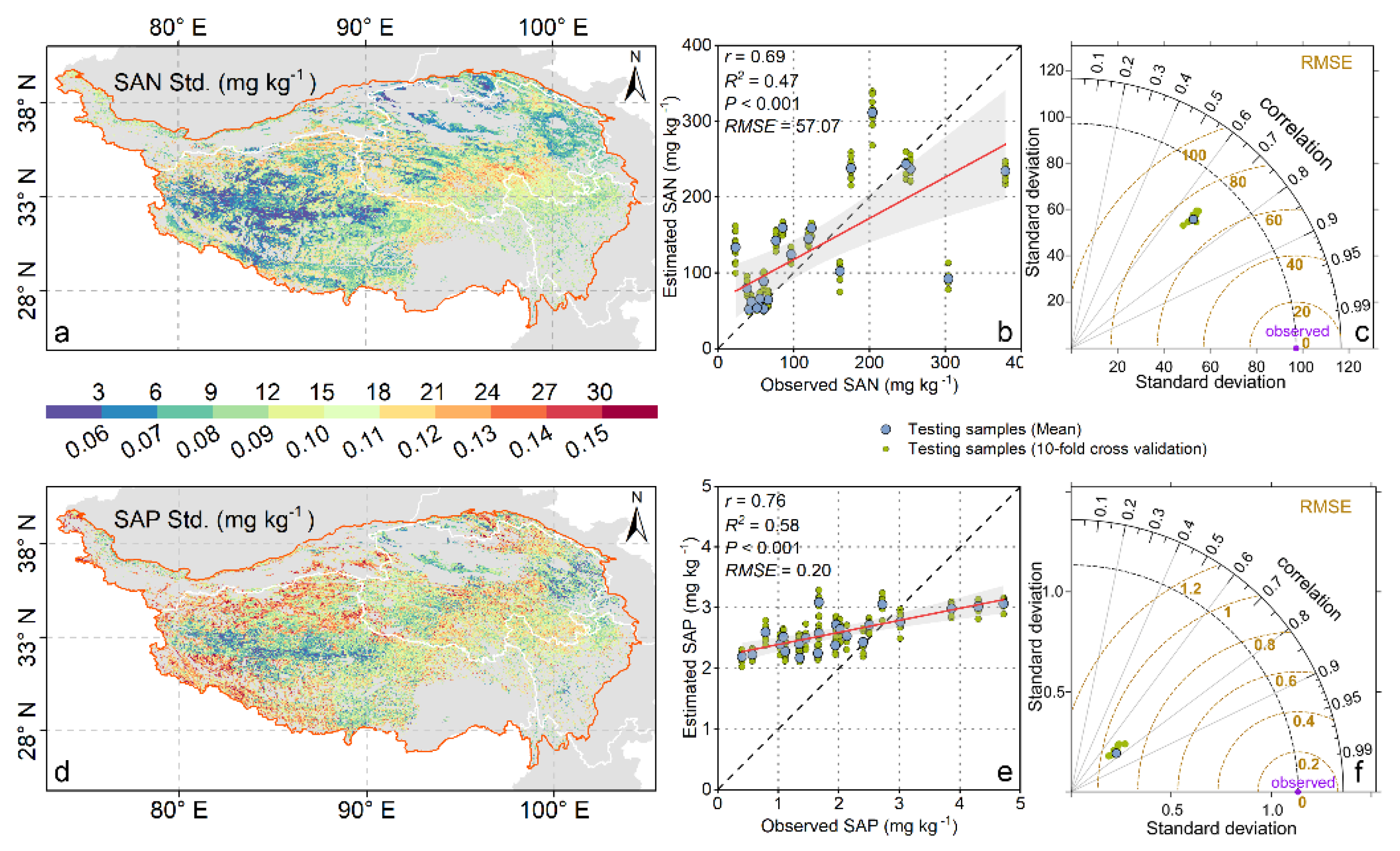
3.1. Results and Evaluation of Random Forest Modeling

We screened 14 environmental covariates for RF modeling (Figure 2). These covariates included four categories: climate, geography, soil, and vegetation. Among them, NPP had the lowest TOL (0.117) and the highest VIF (8.512), and Aspect had the highest TOL (0.727) and the lowest VIF (1.376).

During the model validation phase (based on the sampling data in 2015), all test data and model estimation data conformed to the normal distribution. The estimated and observed values of both SAN and SAP were significantly correlated, with correlation coefficients (r) of 0.69 and 0.76 (p < 0.001), respectively. Furthermore, the fitting lines of the estimated and observed values were close to the 1:1 line, with the RMSEs of SAN and SAP equal to 57.07 mg kg⁻¹ and 0.20 mg kg⁻¹, respectively. However, SAP was underestimated at high SAP contents and overestimated at low SAP contents (Figure 3b,c,e,f).

Based on the 10-fold cross-validation, we determined the uncertainties (robustness) of the SAN and SAP. The estimation errors for each cross-validation are small (with RMSE less than 72.42 mg kg⁻¹ and 1.14 mg kg⁻¹ for SAN and SAP, respectively, and R-square greater than 0.67 and 0.70, respectively), which indicates that the established RF models can perform reliable estimations of SAN and SAP. The uncertainties (standard deviations of 10-fold cross-validation) results (Figure 3a,d) indicate that the SAN and SAP estimates are robust in most areas of alpine grasslands across the QZP, and the robustness of the estimates mainly benefits from the sampling unbiasedness (extensive sampling was conducted in the Tibetan Plateau alpine steppe and alpine meadow, Figure 1). However, the accessibility of some regions limits field sampling, leading to high uncertainties in SAN and SAP estimates, such as in northern Tibet (Qiangtang uninhabited areas) and the Sanjiangyuan regions. In addition, the high uncertainties of SAP estimates also occurred in the southwest of Tibet and Qilian Mountains. Overall, the average uncertainties of SAN and SAP estimates are 11.64 mg kg⁻¹ and 0.10 mg kg⁻¹, respectively, and comparatively the robustness of SAN estimates is higher than that of the SAP estimates.

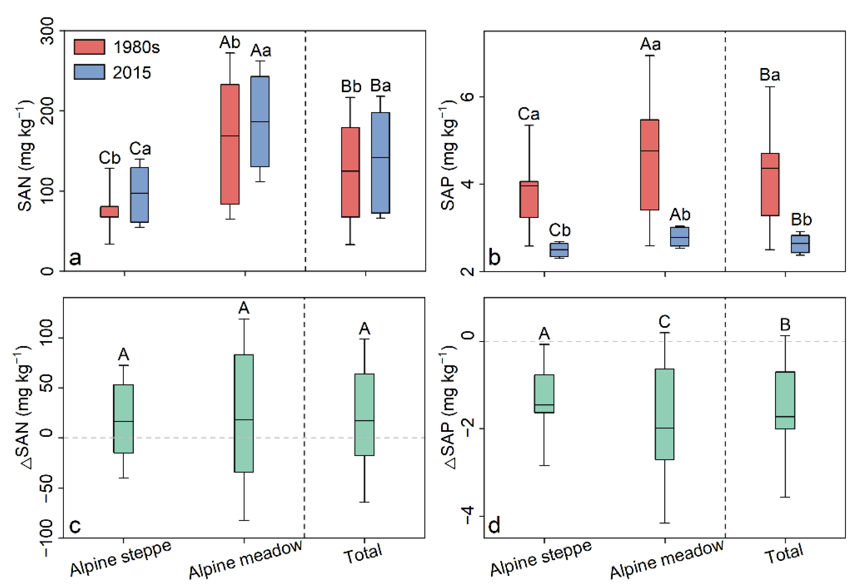
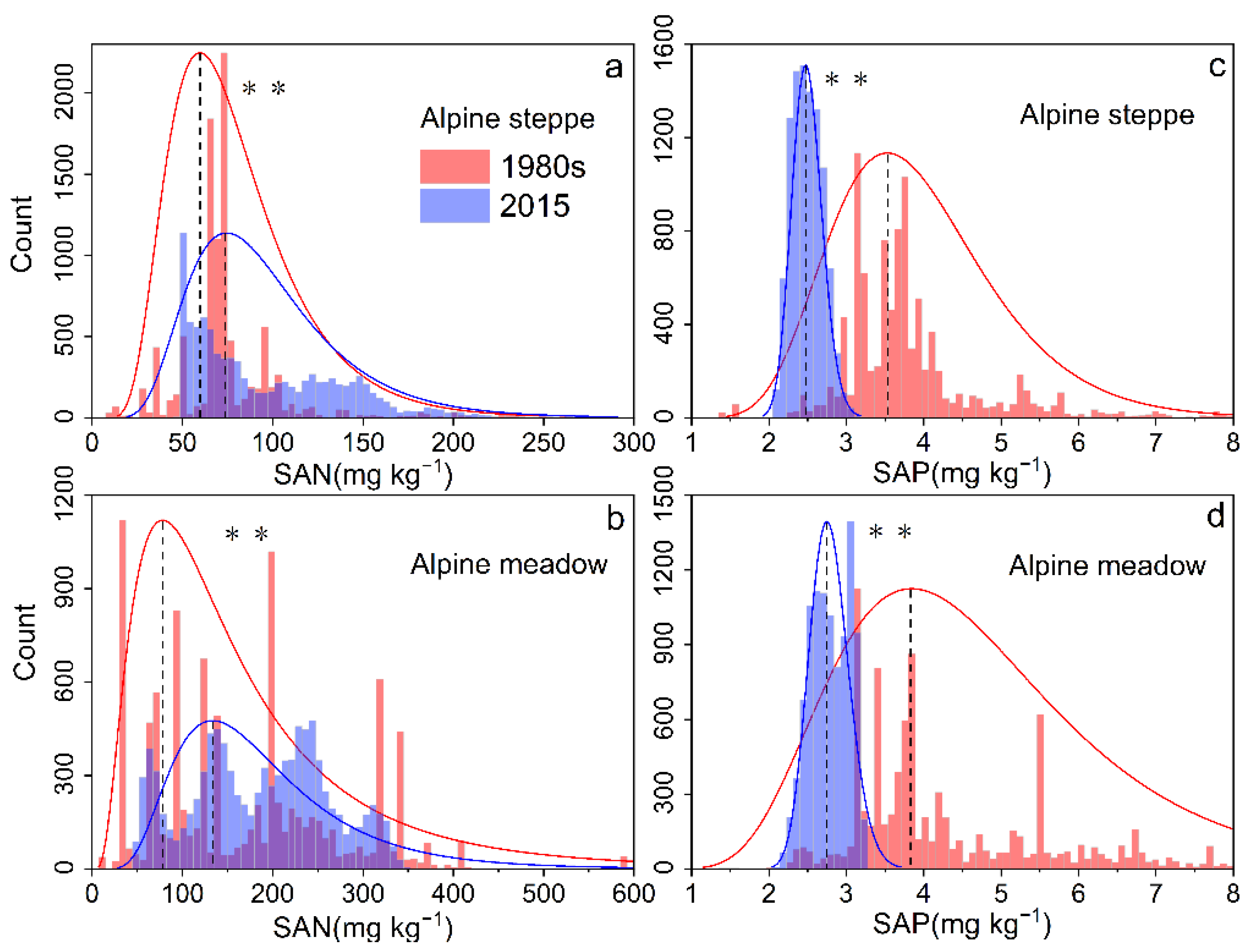
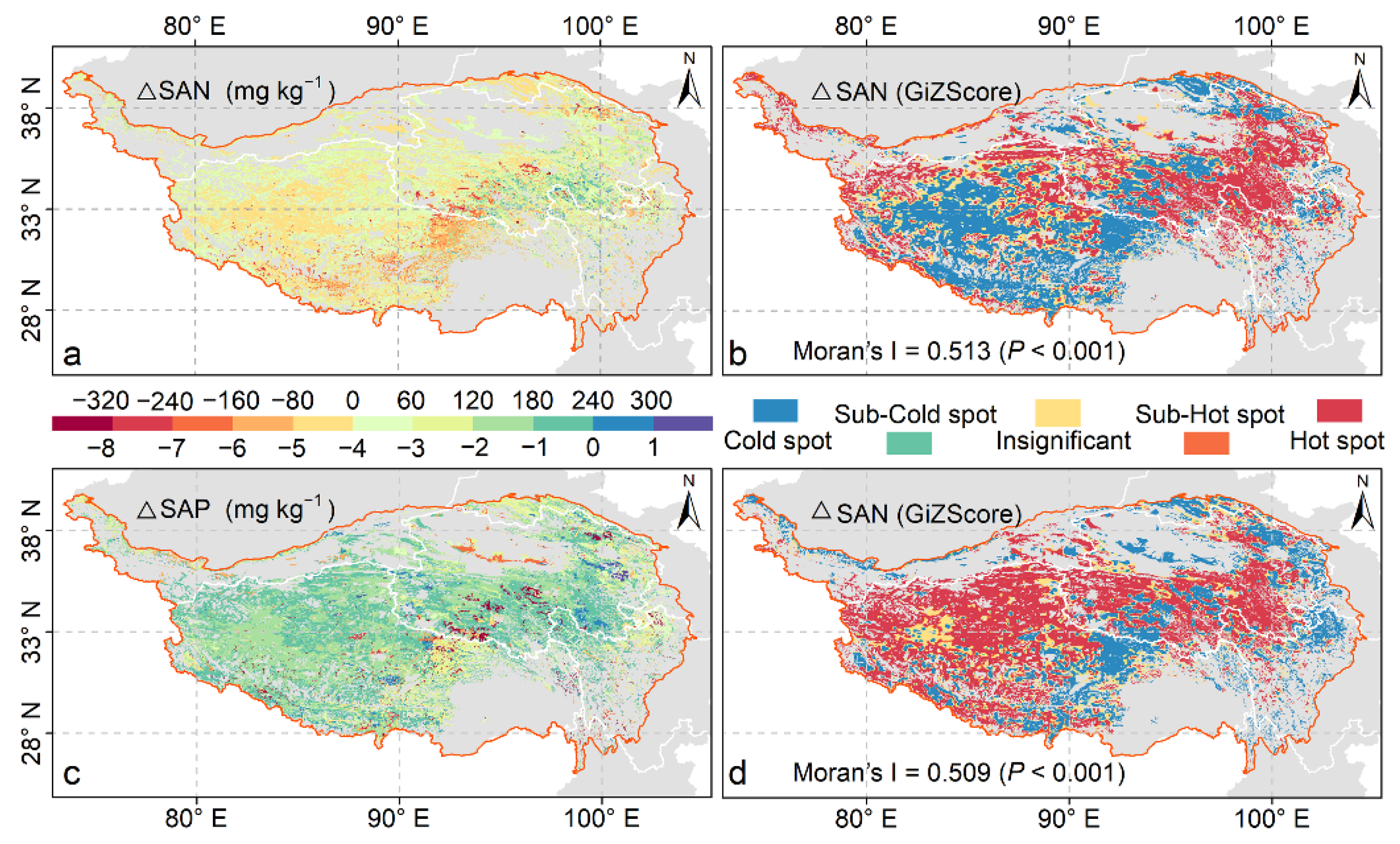
3.2. Spatiotemporal Patterns of SAN and SAP

The estimated SAN and SAP exhibit similar spatial patterns in 2015 (high in the east and low in the west, Figure 4a,c). The SAN and SAP estimates have high global spatial autocorrelation, with the Moran’s I of 0.863 (p < 0.001) and 0.855 (p < 0.001), respectively. Moreover, combined with local spatial autocorrelation analysis (Getis-ord Gi* Index), the SAN and SAP estimates show obvious aggregated distribution characteristics (Figure 4b,d). The hot spot areas (high-value aggregation) are mainly situated in the eastern alpine meadow, such as the Sanjiangyuan regions and the western Sichuan plateau. In addition, the cold spot areas (low-value aggregation) are mainly located in the western alpine steppe, such as the Ali regions and the uninhabited areas of Qiangtang.

The means of SAN and SAP in 2015 for QZP alpine grasslands were 139.96 mg kg⁻¹ and 2.63 mg kg⁻¹, respectively. Compared with SAN and SAP during the 1980s, SAN significantly increased by 18.12 mg kg⁻¹ (SAN, 14.83%, p < 0.05), while SAP decreased significantly by 1.71 mg kg⁻¹ (SAP, 39.40%, p < 0.05) (Figure 5). The contents and dynamics of SAN and SAP presented remarkable differences between alpine steppe and alpine meadow (Figure 6). The means of SAN for alpine steppe and alpine meadow in 2015 were 97.85 mg kg⁻¹ (SAN_steppe) and 186.97 mg kg⁻¹ (SAN_meadow), respectively, and both of them showed significantly increasing trends (p < 0.05), with increases of 17.69 mg kg⁻¹ (22.11%) and 18.58 mg kg⁻¹ (11.04%), respectively, compared to the 1980s (Figure 5a,c and Figure 6a,c). Meanwhile, the means of SAP for alpine steppe and alpine meadow in 2015 were 2.50 mg kg⁻¹ (SAP_steppe) and 2.78 mg kg⁻¹ (SAP_steppe), respectively, and both of them significantly decreased (p < 0.05) by 1.46 mg kg⁻¹ (36.87%) and 1.98 mg kg⁻¹ (41.50%), respectively (Figure 5b,d and Figure 6b,d). Interestingly, the difference in increased values between SAN_steppe and SAN_meadow was not significant (p < 0.05) (Figure 5c), while the decrease in SAP_steppe was significantly lower than that of SAP_meadow (p < 0.05) (Figure 5d). Furthermore, we found synergism between SAN and SAP (r equals 0.77 for alpine steppe and r equals 0.78 for alpine meadow, p < 0.001) (Figure 7a), and the synergism also occurred between ΔSAN and ΔSAP (r equals 0.45 for alpine steppe and r equals 0.54 for alpine meadow, p < 0.001) (Figure 7b).

The spatial distribution of ΔSAN and ΔSAP showed heterogeneous geographical patterns for SAN and SAP dynamics (Figure 8a,c). Spatially, 60% of the alpine grasslands on the QZP showed an increase in SAN and 96% showed a decrease in SAP. Overall, the dynamics of SAN and SAP showed a certain degree of spatial correlation, with the Moran’s I of 0.513 (p < 0.001) and 0.509 (p < 0.001), respectively. Additionally, the local spatial autocorrelation of ΔSAN and ΔSAP was obvious, but the distribution of cold and hot spots exhibited spatial heterogeneity (Figure 8b,d). The hot spots (high-value aggregation) of ΔSAN are mainly located in the northern part of Ali, north of Shuanghu, Sanjiangyuan, and Qinghai Lake, and the cold spots (low-value aggregation) are mainly found in the central part of Ali, Shigatse, western Naqu, and Qilian Mountains, etc. The hot spots of ΔSAP are mainly distributed in Qiangtang, Ali, Cocosili, and Sanjiangyuan, while the cold spots are mainly located in the western part of Naqu, Qilian Mountains, and northern Sichuan.

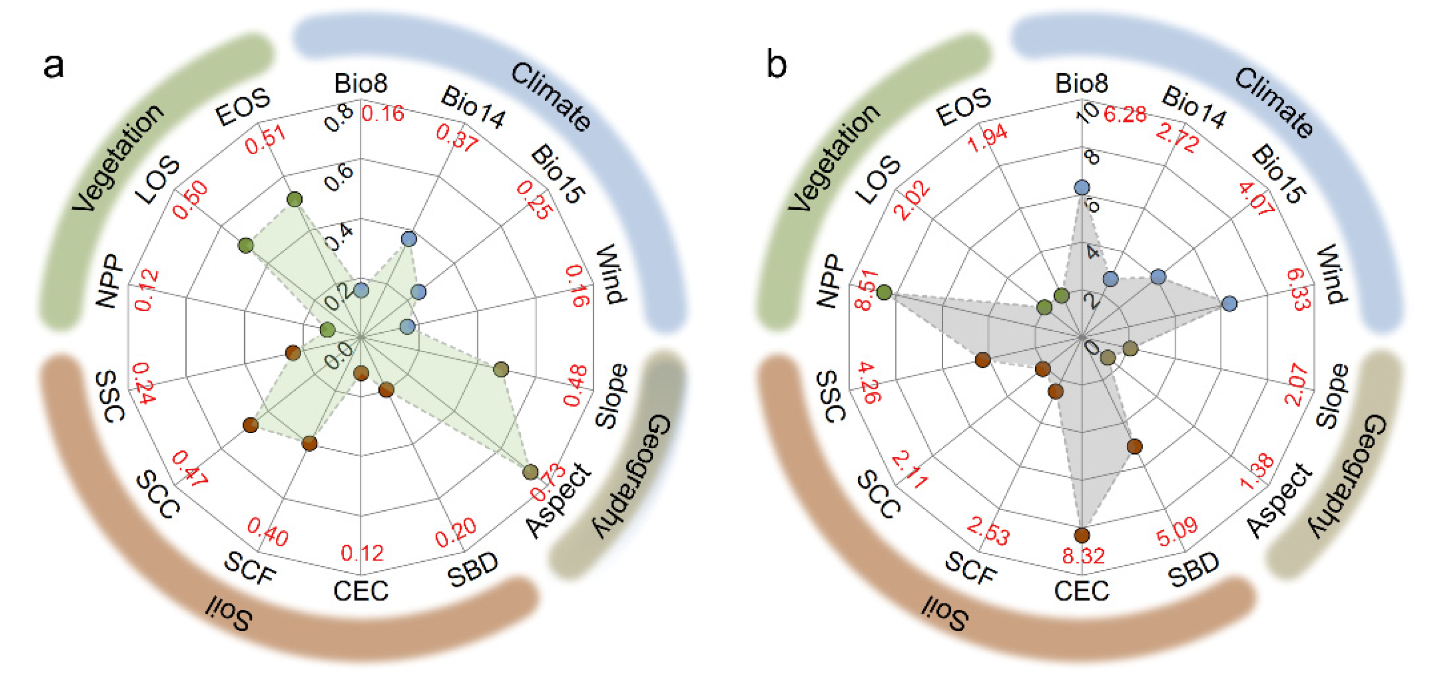
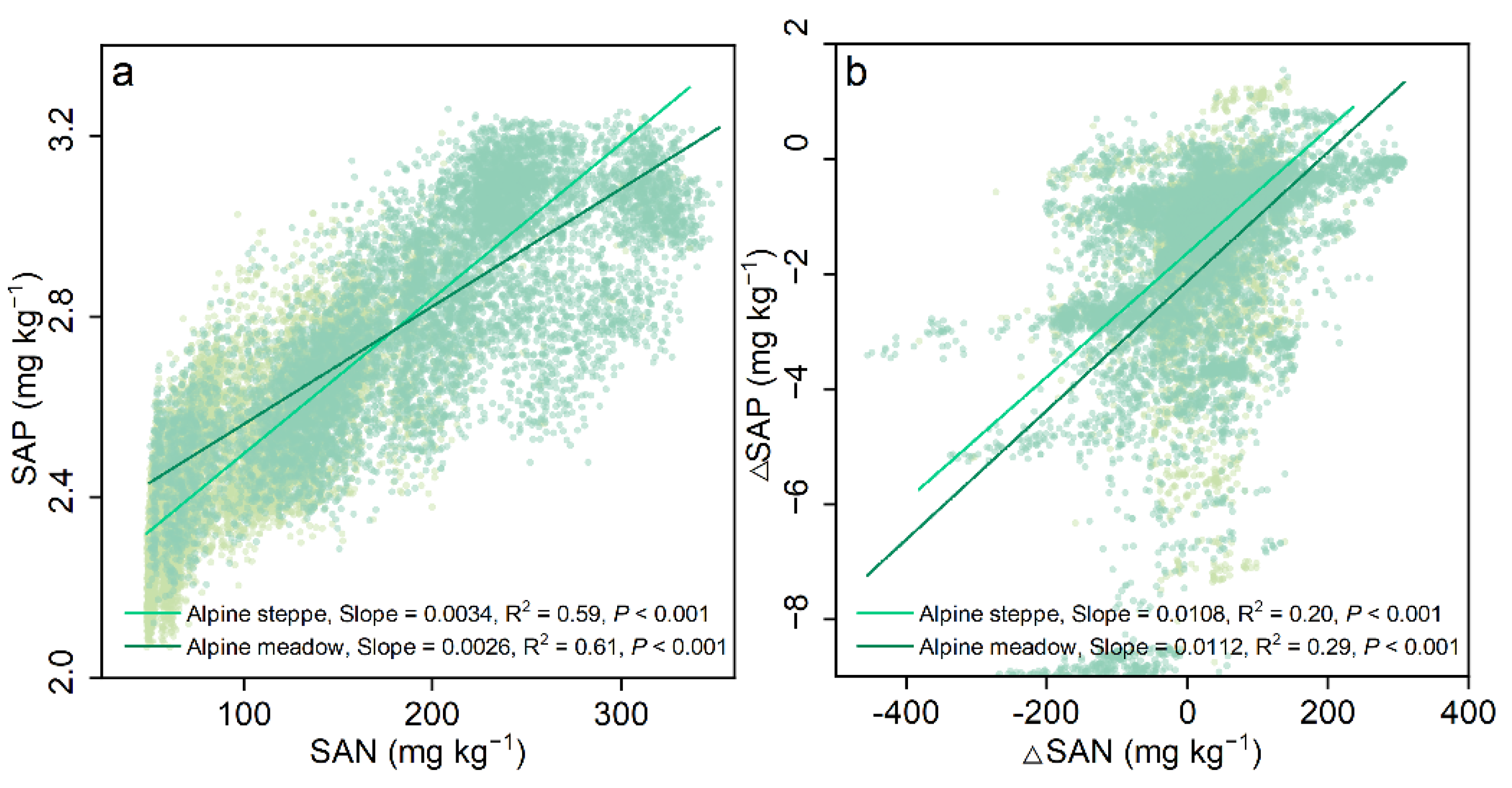
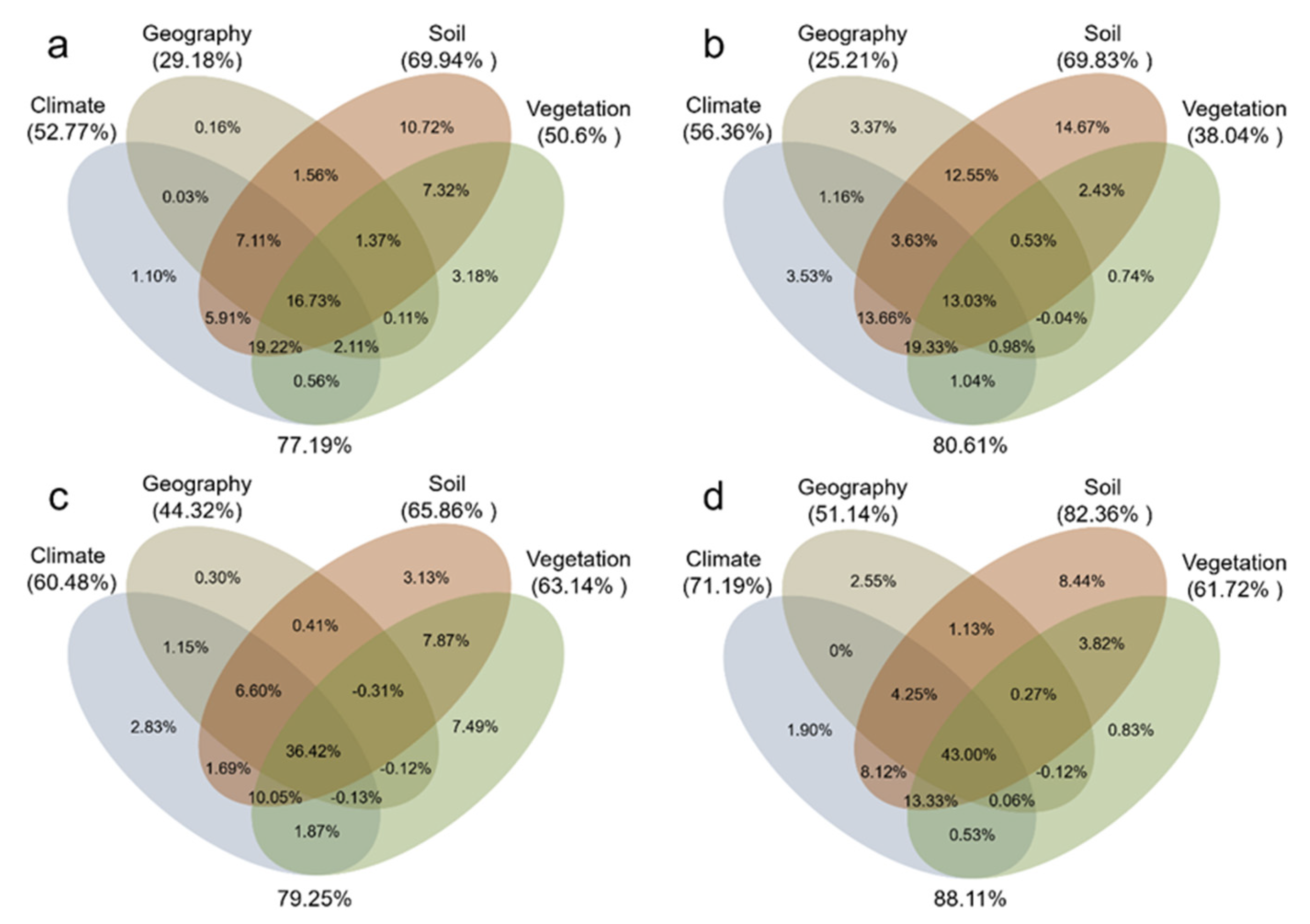
3.3. Effects of Environmental Factors on SAN and SAP

The relative contributions of the 44 environmental drivers (in 4 categories) for the SAN and SAP spatial patterns in different grassland types are shown in Figure 9. Overall, all environmental factors explicitly explained the SAN and SAP spatial variations, with total explanation rates of 77.19% for SAN_steppe (Figure 9a), 80.61% for SAP_steppe (Figure 9b), 79.25% for SAN_meadow (Figure 9c), and 88.11% for SAP_meadow (Figure 9d), respectively. The soil factors had the strongest explanatory rate for the SAN and SAP spatial patterns, followed by climate change, vegetation conditions, and geography factors. Furthermore, we found that the explanation of environmental factors to SAN_meadow and SAP_meadow were always higher than those of SAN_steppe and SAP_steppe.

4. Discussion

Our research mapped the spatial patterns of SAN and SAP in alpine grasslands across the QZP in 2015, with a geographic pattern of higher in the east and lower in the west (higher in alpine meadows and lower in alpine steppes). In general, the SAN content increased significantly, while the SAP content decreased significantly since 1980s. The contents and dynamics of SAN and SAP in alpine meadows and alpine steppes were heterogeneous and were controlled by the interaction between multiple environmental factors, of which the soil physicochemical properties were the dominant factors.

4.1. Evaluation of Model Performance and Results

As we know, environmental factors govern the patterns and dynamics of SAN and SAP. The simulated results (Figure 3) show a significant linear correlation with the in situ observations, which suggests a good model performance in estimating SAN and SAP contents with high robustness in most areas of the QZP. Nevertheless, we identified an overestimation of SAP at low SAP contents and an underestimation at high SAP contents. It might be caused by the instability of SAP in soils [67], which also led to relatively lower robustness in estimates of SAP compared to SAN. Moreover, high uncertainties in regions such as northern Tibet and Sanjiangyuan were due to the accessibility of sampling. Even so, in contrast to the previous empirical models for inversion, which usually include fewer drivers [18,68,69], our RF model (machine learning) involves most of the major drivers and provides more systematic and accurate estimations of SAN and SAP.

The mean SAN and SAP contents of the QZP were 139.96 mg kg⁻¹ and 2.63 mg kg⁻¹, respectively. In addition, the spatial pattern of SAN and SAP estimated in our study was in agreement with previous research [70]. As for the range and magnitude of the data, a site-based study of Mao et al. [71] indicated that the topsoil SAN content of the QZP permafrost zone is about 50 mg kg⁻¹, and this is smaller than our estimate, which is probably because nitrogen is mainly present as organic matter in the permafrost zone and the amount decomposed into SAN is small [31]. However, Wu et al.’s [72] study on fencing and grazing pointed out that the contents of SAN and SAP in alpine meadows of the eastern QZP were about 0.025% (250 mg kg⁻¹) and 2.6 ppm (2.6 mg kg⁻¹), which is comparable to our study. Importantly, the discrepancy between our estimates and other studies may be mainly caused by the different timing and locations of sampling. It has been demonstrated that the ratio of nitrogen and phosphorus always maintains in a certain range during the nitrogen–phosphorus cycle [73]. Moreover, nutrient fixation is limited by the availability of other nutrients in many ecosystems [9]. Consequently, we concluded that the spatial patterns of SAN and SAP present strong consistency (Figure 4 and Figure 7). In addition, we found a significant increment of 18.12 mg kg⁻¹ (14.83%) in SAN and a remarkable decrement of 1.71 mg kg⁻¹ (39.40%) in SAP on the QZP compared with the 1980s. Furthermore, the increase in SAN and the decrease in SAP might lead to a weakening of nitrogen limitation and an intensification of phosphorus limitation, especially in alpine meadows, which was supported by several previous studies [18,73,74].

4.2. Environmental Factors Controlling SAN and SAP

Variations in SAN and SAP present significant differences between the 1980s and 2015 across the QZP (Figure 6, p < 0.01), which can be explained by the different environmental drivers (e.g., climate, geography, soil, and vegetation) (Figure 9). Soil properties are the most important factors, explaining about 80% of the spatial variation in SAN and SAP (Figure 9). Soil moisture and texture perform critical roles in the soil nutrient cycle. Specifically, soil moisture can affect vegetation productivity and regulate soil pH [75,76], and soil texture can influence community structure and soil moisture-holding capacity [77], hence the soil available nutrient contents. It is worth noting that previous reports suggest that parent material may be a critical factor of the global scale soil phosphorus pool [30,78], and the differences between SAP_steppe and SAP_meadow can be explained by the differences in their soil parent materials.

Climate change affects the dynamics of SAN and SAP directly or indirectly. Elevated temperature and precipitation have been shown to enhance microbial activities [79,80,81] and increase the rates of mineralization, nitrification, and denitrification [81,82]. In addition, climate change also alters the weathering rates of parent materials [83,84] and vegetation productivity [85], thereby affecting soil nutrient availability. Our findings demonstrated that the SAN and SAP were higher in alpine meadows than in alpine steppes, since the hydrothermal conditions were more suitable in alpine meadows [49]. Meanwhile, the continuous improvement of hydrothermal conditions on the QZP [86] might be an important reason for the increasing SAN. Moreover, the stored soil nutrients could be released from permafrost thawing due to climate warming, which could affect the SAN and SAP content [15,37]. Additionally, the enhanced atmospheric nitrogen deposition could also raise the SAN [44,87]. The increased precipitation might reduce the weathering rate of phosphorus [83], and heavy precipitation might intensify phosphorus leaching [81], causing the loss of SAP. In addition, this critical biogeochemical process could result in the decrease in SAP, especially in alpine meadows.

The availability of soil nutrients is closely related to vegetation status. Vegetation productivity directly regulates the SAN and SAP contents [88]. In detail, the input of litter could modify soil organic matter content and microbial decomposition processes [89], and thus affect the SAN and SAP contents. Additionally, plant root exudates showed positive effects on soil nutrient mobility and availability [90]. According to previous studies, soil nitrogen increased with the increase in vegetation NDVI and net primary productivity (NPP), while soil phosphorus was not significantly related to vegetation status [91,92]. The changing tendency of soil available nutrients agrees with the variations of soil total nitrogen and phosphorous (Figure S1). Furthermore, alpine meadows have more abundant carbohydrates to meet the high energy demand of available nitrogen and phosphorous [9,93], which leads to a higher SAN_meadow compared to the SAN_steppe. Currently, NPP and NDVI exhibited increasing trends in most parts of alpine grasslands on the QZP [93,94], which could result in an increased SAN. However, the increase in SAN promotes the uptake of SAP by vegetation [95], and the SAP could not be replenished in a timely manner by the weathering of parent material [67], which may be a key reason for the decrease in SAP in the QZP.

Geographic features cannot be ignored due to their effects on SAN and SAP. It has been noted that the soil stoichiometry ratio shows a linear relationship with elevation, and soil nitrogen limitation increases with elevation [30,92]. In addition, geographical-feature-induced temperature variations, water availability, and vegetation differences have significant effects on soil nutrients [96,97].

4.3. Uncertainties and Limitations

Uncertainties and limitations exist when mapping the spatiotemporal patterns of SAN and SAP of the QZP at the regional scale and exploring the underlying mechanisms in this study. Firstly, although comprehensive and sufficient environmental factors were taken into in RF modeling, there might have some biases when applying the global-scaled datasets, such as climate and soil data, to the regional-scaled analysis [98,99]. Secondly, the samplings in the depopulated zone were relatively sparse, which also brought uncertainty to our study. Thirdly, the vegetation types of 2000 used in this study could not accurately reflect the distribution of alpine meadows and alpine steppes across the QZP in the 1980s and 2015 [100], which might influence the accuracy of the research to some extent. Fourthly, it was difficult to obtain the data of atmospheric nitrogen deposition [44], microbial activities [101,102], and litter stoichiometry [103] across regional areas, which could result in either overestimating or underestimating the actual value. Finally, ecological conservation projects such as fencing, grazing prohibitions, and artificial grasslands could substantially affect the dynamics of soil available nutrients [27,104]. In general, sufficient effective indicators should be considered to mine the driving mechanisms of SAN and SAP at the regional scale, and long-term observation is necessary for future research. Meanwhile, as global changes affect the dynamics of SAN and SAP, controls to cope with changes in nitrogen and phosphorus limitation should be considered in future studies.

5. Conclusions

In this study, we estimated the patterns and dynamics of SAN and SAP contents in alpine grasslands across the QZP based on RF models and revealed the integrated impact mechanisms of environmental factors on SAN and SAP contents and patterns. Our research indicated that the mean SAN and SAP contents of alpine grasslands on the Tibetan Plateau were 139.96 mg kg⁻¹ and 2.63 mg kg⁻¹, respectively, in 2015, with a significant increase in SAN and a significant decrease in SAP contents since the 1980s, and the patterns and dynamics of SAN and SAP varied considerably among alpine meadows and alpine steppes. These results suggested that in the context of global change the nutrient limitation might shift from nitrogen limitation to phosphorus limitation in alpine grasslands across the QZP, especially in alpine meadows. Furthermore, redundancy analysis revealed that the interactions between multiple environmental elements controlled the patterns of SAN and SAP, and the soil physicochemical properties were the dominating factors. Overall, our research provided new insights into the patterns and dynamics of SAN and SAP at the regional scale and provided important scientific support for alpine grasslands across the QZP to cope with the future environmental changes and to optimize sustainable management.

References

1. Van der Putten, W.H.; Bardgett, R.D.; Bever, J.D.; Bezemer, T.M.; Casper, B.B.; Fukami, T.; Kardol, P.; Klironomos, J.N.; Kulmatiski, A.; Schweitzer, J.A. Plant–soil feedbacks: The past, the present and future challenges. J. Ecol. 2013, 101, 265–276. [Google Scholar] [CrossRef]
2. Sistla, S.A.; Schimel, J.P. Stoichiometric flexibility as a regulator of carbon and nutrient cycling in terrestrial ecosystems under change. New Phytol. 2012, 196, 68–78. [Google Scholar] [CrossRef] [PubMed]
3. Craine, J.M.; Dybzinski, R. Mechanisms of plant competition for nutrients, water and light. Funct. Ecol. 2013, 27, 833–840. [Google Scholar] [CrossRef]
4. Fang, Z.; Li, D.-D.; Jiao, F.; Yao, J.; Du, H.-T. The latitudinal patterns of leaf and soil C: N: P stoichiometry in the loess plateau of China. Front. Plant Sci. 2019, 10, 85. [Google Scholar] [CrossRef] [PubMed] [Green Version]
5. Norouzi, M.; Ayoubi, S.; Jalalian, A.; Khademi, H.; Dehghani, A. Predicting rainfed wheat quality and quantity by artificial neural network using terrain and soil characteristics. Acta Agric. Scand. Sect. B—Soil Plant Sci. 2010, 60, 341–352. [Google Scholar] [CrossRef]
6. Fernández-Martínez, M.; Vicca, S.; Janssens, I.A.; Sardans, J.; Luyssaert, S.; Campioli, M.; Chapin, F.S., III; Ciais, P.; Malhi, Y.; Obersteiner, M. Nutrient availability as the key regulator of global forest carbon balance. Nat. Clim. Change 2014, 4, 471–476. [Google Scholar] [CrossRef] [Green Version]
7. Terrer, C.; Jackson, R.B.; Prentice, I.C.; Keenan, T.F.; Kaiser, C.; Vicca, S.; Fisher, J.B.; Reich, P.B.; Stocker, B.D.; Hungate, B.A. Nitrogen and phosphorus constrain the CO2 fertilization of global plant biomass. Nat. Clim. Change 2019, 9, 684–689. [Google Scholar] [CrossRef] [Green Version]
8. Wieder, W.R.; Cleveland, C.C.; Smith, W.K.; Todd-Brown, K. Future productivity and carbon storage limited by terrestrial nutrient availability. Nat. Geosci. 2015, 8, 441–444. [Google Scholar] [CrossRef]
9. Chapin, F.S.; Matson, P.A.; Mooney, H.A.; Vitousek, P.M. Principles of Terrestrial Ecosystem Ecology; Springer: New York, NY, USA, 2011. [Google Scholar]
10. Delgado-Baquerizo, M.; Maestre, F.T.; Gallardo, A.; Bowker, M.A.; Wallenstein, M.D.; Quero, J.L.; Ochoa, V.; Gozalo, B.; García-Gómez, M.; Soliveres, S. Decoupling of soil nutrient cycles as a function of aridity in global drylands. Nature 2013, 502, 672–676. [Google Scholar] [CrossRef]
11. Geng, Y.; Baumann, F.; Song, C.; Zhang, M.; Shi, Y.; Kühn, P.; Scholten, T.; He, J.-S. Increasing temperature reduces the coupling between available nitrogen and phosphorus in soils of Chinese grasslands. Sci. Rep. 2017, 7, 43524. [Google Scholar] [CrossRef]
12. Du, E.; Terrer, C.; Pellegrini, A.F.; Ahlström, A.; van Lissa, C.J.; Zhao, X.; Xia, N.; Wu, X.; Jackson, R.B. Global patterns of terrestrial nitrogen and phosphorus limitation. Nat. Geosci. 2020, 13, 221–226. [Google Scholar] [CrossRef]
13. Hou, E.; Luo, Y.; Kuang, Y.; Chen, C.; Lu, X.; Jiang, L.; Luo, X.; Wen, D. Global meta-analysis shows pervasive phosphorus limitation of aboveground plant production in natural terrestrial ecosystems. Nat. Commun. 2020, 11, 637. [Google Scholar] [CrossRef] [PubMed] [Green Version]
14. Kou, D.; Yang, G.; Li, F.; Feng, X.; Zhang, D.; Mao, C.; Zhang, Q.; Peng, Y.; Ji, C.; Zhu, Q. Progressive nitrogen limitation across the Tibetan alpine permafrost region. Nat. Commun. 2020, 11, 3331. [Google Scholar] [CrossRef] [PubMed]
15. Yang, G.; Peng, Y.; Abbott, B.W.; Biasi, C.; Wei, B.; Zhang, D.; Wang, J.; Yu, J.; Li, F.; Wang, G. Phosphorus rather than nitrogen regulates ecosystem carbon dynamics after permafrost thaw. Glob. Change Biol. 2021, 27, 5818–5830. [Google Scholar] [CrossRef]
16. Jeong, G.; Oeverdieck, H.; Park, S.J.; Huwe, B.; Ließ, M. Spatial soil nutrients prediction using three supervised learning methods for assessment of land potentials in complex terrain. Catena 2017, 154, 73–84. [Google Scholar] [CrossRef]
17. Xu, L.; Yu, G.; He, N.; Wang, Q.; Gao, Y.; Wen, D.; Li, S.; Niu, S.; Ge, J. Carbon storage in China’s terrestrial ecosystems: A synthesis. Sci. Rep. 2018, 8, 2806. [Google Scholar] [CrossRef] [Green Version]
18. Yang, Y.; Fang, J.; Ji, C.; Datta, A.; Li, P.; Ma, W.; Mohammat, A.; Shen, H.; Hu, H.; Knapp, B.O.; et al. Stoichiometric shifts in surface soils over broad geographical scales: Evidence from China’s grasslands. Glob. Ecol. Biogeogr. 2014, 23, 947–955. [Google Scholar] [CrossRef]
19. Yang, Y.; Fang, J.; Smith, P.; Tang, Y.; Chen, A.; Ji, C.; Hu, H.; Rao, S.; Tan, K.; He, J.S. Changes in topsoil carbon stock in the Tibetan grasslands between the 1980s and 2004. Glob. Change Biol. 2009, 15, 2723–2729. [Google Scholar] [CrossRef]
20. Stockmann, U.; Adams, M.A.; Crawford, J.W.; Field, D.J.; Henakaarchchi, N.; Jenkins, M.; Minasny, B.; McBratney, A.B.; De Courcelles, V.D.R.; Singh, K. The knowns, known unknowns and unknowns of sequestration of soil organic carbon. Agric. Ecosyst. Environ. 2013, 164, 80–99. [Google Scholar] [CrossRef]
21. Zhang, F.; Wang, Z.; Glidden, S.; Wu, Y.; Tang, L.; Liu, Q.; Li, C.; Frolking, S. Changes in the soil organic carbon balance on China’s cropland during the last two decades of the 20th century. Sci. Rep. 2017, 7, 7144. [Google Scholar] [CrossRef]
22. Zeraatpisheh, M.; Ayoubi, S.; Jafari, A.; Tajik, S.; Finke, P. Digital mapping of soil properties using multiple machine learning in a semi-arid region, central Iran. Geoderma 2019, 338, 445–452. [Google Scholar] [CrossRef]
23. Zeraatpisheh, M.; Ayoubi, S.; Mirbagheri, Z.; Mosaddeghi, M.R.; Xu, M. Spatial prediction of soil aggregate stability and soil organic carbon in aggregate fractions using machine learning algorithms and environmental variables. Geoderma Reg. 2021, 27, e00440. [Google Scholar] [CrossRef]
24. Naimi, S.; Ayoubi, S.; Demattê, J.A.; Zeraatpisheh, M.; Amorim, M.T.A.; Mello, F.A.D.O. Spatial prediction of soil surface properties in an arid region using synthetic soil image and machine learning. Geocarto Int. 2021, 1–24. [Google Scholar] [CrossRef]
25. Azizi, K.; Ayoubi, S.; Nabiollahi, K.; Garosi, Y.; Gislum, R. Predicting heavy metal contents by applying machine learning approaches and environmental covariates in west of Iran. J. Geochem. Explor. 2022, 233, 106921. [Google Scholar] [CrossRef]
26. Hengl, T.; Mendes de Jesus, J.; Heuvelink, G.B.; Ruiperez Gonzalez, M.; Kilibarda, M.; Blagotić, A.; Shangguan, W.; Wright, M.N.; Geng, X.; Bauer-Marschallinger, B. SoilGrids250m: Global gridded soil information based on machine learning. PLoS ONE 2017, 12, e0169748. [Google Scholar] [CrossRef] [Green Version]
27. Li, H.W.; Wu, Y.P.; Liu, S.G.; Xiao, J.F.; Zhao, W.Z.; Chen, J.; Alexandrov, G.; Cao, Y. Decipher soil organic carbon dynamics and driving forces across China using machine learning. Glob. Change Biol. 2022, 28, 3394–3410. [Google Scholar] [CrossRef] [PubMed]
28. Brungard, C.W.; Boettinger, J.L.; Duniway, M.C.; Wills, S.A.; Edwards, T.C., Jr. Machine learning for predicting soil classes in three semi-arid landscapes. Geoderma 2015, 239, 68–83. [Google Scholar] [CrossRef] [Green Version]
29. Padarian, J.; Minasny, B.; McBratney, A.B. Machine learning and soil sciences: A review aided by machine learning tools. Soil 2020, 6, 35–52. [Google Scholar] [CrossRef] [Green Version]
30. Augusto, L.; Achat, D.L.; Jonard, M.; Vidal, D.; Ringeval, B. Soil parent material—A major driver of plant nutrient limitations in terrestrial ecosystems. Glob. Change Biol. 2017, 23, 3808–3824. [Google Scholar] [CrossRef]
31. Binkley, D.; Fisher, R.F. Ecology and Management of Forest Soils; John Wiley & Sons: Hoboken, NJ, USA, 2019. [Google Scholar]
32. Brady, N.C.; Weil, R.R. Elements of the Nature and Properties of Soils; Pearson Prentice Hall: Upper Saddle River, NJ, USA, 2010. [Google Scholar]
33. Matias, L.; Castro, J.; Zamora, R. Soil-nutrient availability under a global-change scenario in a Mediterranean mountain ecosystem. Glob. Change Biol. 2011, 17, 1646–1657. [Google Scholar] [CrossRef]
34. Peñuelas, J.; Poulter, B.; Sardans, J.; Ciais, P.; Van Der Velde, M.; Bopp, L.; Boucher, O.; Godderis, Y.; Hinsinger, P.; Llusia, J. Human-induced nitrogen–phosphorus imbalances alter natural and managed ecosystems across the globe. Nat. Commun. 2013, 4, 2934. [Google Scholar] [CrossRef] [PubMed] [Green Version]
35. Wardle, D.A. Drivers of decoupling in drylands. Nature 2013, 502, 628–629. [Google Scholar] [CrossRef] [PubMed] [Green Version]
36. Keuper, F.; Dorrepaal, E.; van Bodegom, P.M.; van Logtestijn, R.; Venhuizen, G.; van Hal, J.; Aerts, R. Experimentally increased nutrient availability at the permafrost thaw front selectively enhances biomass production of deep-rooting subarctic peatland species. Glob. Change Biol. 2017, 23, 4257–4266. [Google Scholar] [CrossRef] [PubMed]
37. Salmon, V.G.; Soucy, P.; Mauritz, M.; Celis, G.; Natali, S.M.; Mack, M.C.; Schuur, E.A. Nitrogen availability increases in a tundra ecosystem during five years of experimental permafrost thaw. Glob. Change Biol. 2016, 22, 1927–1941. [Google Scholar] [CrossRef] [PubMed]
38. Conant, R.T.; Ryan, M.G.; Ågren, G.I.; Birge, H.E.; Davidson, E.A.; Eliasson, P.E.; Evans, S.E.; Frey, S.D.; Giardina, C.P.; Hopkins, F.M. Temperature and soil organic matter decomposition rates–synthesis of current knowledge and a way forward. Glob. Change Biol. 2011, 17, 3392–3404. [Google Scholar] [CrossRef]
39. Durán, J.; Morse, J.L.; Groffman, P.M.; Campbell, J.L.; Christenson, L.M.; Driscoll, C.T.; Fahey, T.J.; Fisk, M.C.; Likens, G.E.; Melillo, J.M. Climate change decreases nitrogen pools and mineralization rates in northern hardwood forests. Ecosphere 2016, 7, e01251. [Google Scholar] [CrossRef]
40. Mooshammer, M.; Hofhansl, F.; Frank, A.H.; Wanek, W.; Hämmerle, I.; Leitner, S.; Schnecker, J.; Wild, B.; Watzka, M.; Keiblinger, K.M. Decoupling of microbial carbon, nitrogen, and phosphorus cycling in response to extreme temperature events. Sci. Adv. 2017, 3, e1602781. [Google Scholar] [CrossRef] [Green Version]
41. Yue, K.; Fornara, D.A.; Yang, W.; Peng, Y.; Li, Z.; Wu, F.; Peng, C. Effects of three global change drivers on terrestrial C:N:P stoichiometry: A global synthesis. Glob. Change Biol. 2017, 23, 2450–2463. [Google Scholar] [CrossRef]
42. Sasaki, T.; Yoshihara, Y.; Jamsran, U.; Ohkuro, T. Ecological stoichiometry explains larger-scale facilitation processes by shrubs on species coexistence among understory plants. Ecol. Eng. 2010, 36, 1070–1075. [Google Scholar] [CrossRef]
43. Wardle, D.A.; Walker, L.R.; Bardgett, R.D. Ecosystem properties and forest decline in contrasting long-term chronosequences. Science 2004, 305, 509–513. [Google Scholar] [CrossRef]
44. Liu, X.; Zhang, Y.; Han, W.; Tang, A.; Shen, J.; Cui, Z.; Vitousek, P.; Erisman, J.W.; Goulding, K.; Christie, P. Enhanced nitrogen deposition over China. Nature 2013, 494, 459–462. [Google Scholar] [CrossRef] [PubMed]
45. Lü, C.; Tian, H. Spatial and temporal patterns of nitrogen deposition in China: Synthesis of observational data. J. Geophys. Res. Atmos. 2007, 112. [Google Scholar] [CrossRef]
46. Hou, E.; Chen, C.; Luo, Y.; Zhou, G.; Kuang, Y.; Zhang, Y.; Heenan, M.; Lu, X.; Wen, D. Effects of climate on soil phosphorus cycle and availability in natural terrestrial ecosystems. Glob. Change Biol. 2018, 24, 3344–3356. [Google Scholar] [CrossRef] [PubMed] [Green Version]
47. Barrow, N. A mechanistic model for describing the sorption and desorption of phosphate by soil. J. Soil Sci. 1983, 34, 733–750. [Google Scholar] [CrossRef]
48. Sims, J.T.; Simard, R.R.; Joern, B.C. Phosphorus loss in agricultural drainage: Historical perspective and current research. J. Environ. Qual. 1998, 27, 277–293. [Google Scholar] [CrossRef] [Green Version]
49. Sun, J.; Ye, C.; Liu, M.; Wang, Y.; Chen, J.; Wang, S.; Lu, X.; Liu, G.; Xu, M.; Li, R.; et al. Response of net reduction rate in vegetation carbon uptake to climate change across a unique gradient zone on the Tibetan Plateau. Environ. Res. 2022, 203, 111894. [Google Scholar] [CrossRef] [PubMed]
50. Sun, J.; Ma, B.; Lu, X. Grazing enhances soil nutrient effects: Trade-offs between aboveground and belowground biomass in alpine grasslands of the Tibetan Plateau. Land Degrad. Dev. 2018, 29, 337–348. [Google Scholar] [CrossRef]
51. He, J.S.; Wang, L.; Flynn, D.F.B.; Wang, X.P.; Ma, W.H.; Fang, J.Y. Leaf nitrogen: Phosphorus stoichiometry across Chinese grassland biomes. Oecologia 2008, 155, 301–310. [Google Scholar] [CrossRef]
52. Sun, Y.; Liu, S.; Liu, Y.; Dong, Y.; Li, M.; An, Y.; Shi, F.; Beazley, R. Effects of the interaction among climate, terrain and human activities on biodiversity on the Qinghai-Tibet Plateau. Sci. Total Environ. 2021, 794, 148497. [Google Scholar] [CrossRef]
53. Shen, X.; Liu, Y.; Zhang, J.; Wang, Y.; Ma, R.; Liu, B.; Lu, X.; Jiang, M. Asymmetric impacts of diurnal warming on vegetation carbon sequestration of marshes in the Qinghai Tibet Plateau. Glob. Biogeochem. Cycles 2022, 36, e2022GB007396. [Google Scholar] [CrossRef]
54. Sun, J.; Zhou, T.C.; Liu, M.; Chen, Y.C.; Liu, G.H.; Xu, M.; Shi, P.L.; Peng, F.; Tsunekawa, A.; Liu, Y.; et al. Water and heat availability are drivers of the aboveground plant carbon accumulation rate in alpine grasslands on the Tibetan Plateau. Glob. Ecol. Biogeogr. 2019, 29, 50–64. [Google Scholar] [CrossRef] [Green Version]
55. Schaefer, C.E.G.R.; Pereira, T.T.C.; Ker, J.C.; Almeida, I.C.C.; Simas, F.N.B.; de Oliveira, F.S.; Correa, G.R.; Vieira, G. Soils and Landforms at Hope Bay, Antarctic Peninsula: Formation, Classification, Distribution, and Relationships. Soil Sci. Soc. Am. J. 2015, 79, 175–184. [Google Scholar] [CrossRef]
56. Zhou, T.C.; Sun, J.; Liu, M.; Shi, P.L.; Zhang, X.B.; Sun, W.; Yang, G.; Tsunekawa, A. Coupling between plant nitrogen and phosphorus along water and heat gradients in alpine grassland. Sci. Total Environ. 2020, 701, 134660. [Google Scholar] [CrossRef]
57. Olsen, S.R. Estimation of Available Phosphorus in Soils by Extraction with Sodium Bicarbonate; US Department of Agriculture: Washington, DC, USA, 1954.
58. Ma, H.; Mo, L.; Crowther, T.W.; Maynard, D.S.; van den Hoogen, J.; Stocker, B.D.; Terrer, C.; Zohner, C.M. The global distribution and environmental drivers of aboveground versus belowground plant biomass. Nat. Ecol. Evol. 2021, 5, 1110–1122. [Google Scholar] [CrossRef] [PubMed]
59. Liu, J.; Wang, J.; Xiong, J.; Cheng, W.; Sun, H.; Yong, Z.; Wang, N. Hybrid Models Incorporating Bivariate Statistics and Machine Learning Methods for Flash Flood Susceptibility Assessment Based on Remote Sensing Datasets. Remote Sens. 2021, 13, 4945. [Google Scholar] [CrossRef]
60. Breiman, L. Random forests. Mach. Learn. 2001, 45, 5–32. [Google Scholar] [CrossRef] [Green Version]
61. Gomes, L.C.; Faria, R.M.; de Souza, E.; Veloso, G.V.; Schaefer, C.E.G.R.; Fernandes, E.I. Modelling and mapping soil organic carbon stocks in Brazil. Geoderma 2019, 340, 337–350. [Google Scholar] [CrossRef]
62. Pedregosa, F.; Varoquaux, G.; Gramfort, A.; Michel, V.; Thirion, B.; Grisel, O.; Blondel, M.; Prettenhofer, P.; Weiss, R.; Dubourg, V. Scikit-learn: Machine learning in Python. J. Mach. Learn. Res. 2011, 12, 2825–2830. [Google Scholar]
63. Longley, P.A.; Goodchild, M.F.; Maguire, D.J.; Rhind, D.W. Geographical Information Systems: Principles, Techniques, Management and Applications. Volume 2: Management Issues and Applications; Wiley: New York, NY, USA, 1999. [Google Scholar]
64. Wang, Y.; Zhang, T.; Yao, S.; Deng, Y. Spatio-temporal Evolution and Factors Influencing the Control Efficiency for Soil and Water Loss in the Wei River Catchment, China. Sustainability 2019, 11, 216. [Google Scholar] [CrossRef] [Green Version]
65. Tang, W.; Zhou, T.; Sun, J.; Li, Y.; Li, W. Accelerated Urban Expansion in Lhasa City and the Implications for Sustainable Development in a Plateau City. Sustainability 2017, 9, 1499. [Google Scholar] [CrossRef] [Green Version]
66. R Core Team. R: A Language and Environment for Statistical Computing; R Foundation for Statistical Computing: Vienna, Austria, 2013. [Google Scholar]
67. Li, Z.L.; Zhang, D.Y.; Peng, Y.F.; Qin, S.Q.; Wang, L.; Hou, E.Q.; Yang, Y.H. Divergent Drivers of Various Topsoil Phosphorus Fractions Across Tibetan Alpine Grasslands. J. Geophys. Res. -Biogeo. 2022, 127, e2022JG006795. [Google Scholar] [CrossRef]
68. Gherardi, L.A.; Sala, O.E. Global patterns and climatic controls of belowground net carbon fixation. Proc. Natl. Acad. Sci. USA 2020, 117, 20038–20043. [Google Scholar] [CrossRef] [PubMed]
69. Mao, D.; Wang, Z.; Li, L.; Ma, W. Spatiotemporal dynamics of grassland aboveground net primary productivity and its association with climatic pattern and changes in Northern China. Ecol. Indic. 2014, 41, 40–48. [Google Scholar] [CrossRef]
70. Shangguan, W.; Dai, Y.; Liu, B.; Zhu, A.; Duan, Q.; Wu, L.; Ji, D.; Ye, A.; Yuan, H.; Zhang, Q. A China data set of soil properties for land surface modeling. J. Adv. Model Earth Syst. 2013, 5, 212–224. [Google Scholar] [CrossRef]
71. Mao, C.; Kou, D.; Chen, L.; Qin, S.; Zhang, D.; Peng, Y.; Yang, Y. Permafrost nitrogen status and its determinants on the Tibetan Plateau. Glob. Change Biol. 2020, 26, 5290–5302. [Google Scholar] [CrossRef]
72. Wu, G.-L.; Du, G.-Z.; Liu, Z.-H.; Thirgood, S. Effect of fencing and grazing on a Kobresia-dominated meadow in the Qinghai-Tibetan Plateau. Plant Soil 2009, 319, 115–126. [Google Scholar] [CrossRef]
73. Güsewell, S. N: P ratios in terrestrial plants: Variation and functional significance. New Phytol. 2004, 164, 243–266. [Google Scholar] [CrossRef]
74. Goll, D.S.; Brovkin, V.; Parida, B.; Reick, C.H.; Kattge, J.; Reich, P.B.; Van Bodegom, P.; Niinemets, Ü. Nutrient limitation reduces land carbon uptake in simulations with a model of combined carbon, nitrogen and phosphorus cycling. Biogeosciences 2012, 9, 3547–3569. [Google Scholar] [CrossRef] [Green Version]
75. Liu, L.; Gudmundsson, L.; Hauser, M.; Qin, D.; Li, S.; Seneviratne, S.I. Soil moisture dominates dryness stress on ecosystem production globally. Nat. Commun. 2020, 11, 4892. [Google Scholar] [CrossRef]
76. Tian, L.; Zhao, L.; Wu, X.; Fang, H.; Zhao, Y.; Yue, G.; Liu, G.; Chen, H. Vertical patterns and controls of soil nutrients in alpine grassland: Implications for nutrient uptake. Sci. Total Environ. 2017, 607, 855–864. [Google Scholar] [CrossRef]
77. Abdu, H.; Robinson, D.; Seyfried, M.; Jones, S.B. Geophysical imaging of watershed subsurface patterns and prediction of soil texture and water holding capacity. Water Resour. Res. 2008, 44. [Google Scholar] [CrossRef]
78. He, X.; Augusto, L.; Goll, D.S.; Ringeval, B.; Wang, Y.; Helfenstein, J.; Huang, Y.; Yu, K.; Wang, Z.; Yang, Y. Global patterns and drivers of soil total phosphorus concentration. Earth Syst. Sci. Data 2021, 13, 5831–5846. [Google Scholar] [CrossRef]
79. Allison, S.D.; Treseder, K.K. Warming and drying suppress microbial activity and carbon cycling in boreal forest soils. Glob. Change Biol. 2008, 14, 2898–2909. [Google Scholar] [CrossRef] [Green Version]
80. Bai, E.; Li, S.; Xu, W.; Li, W.; Dai, W.; Jiang, P. A meta-analysis of experimental warming effects on terrestrial nitrogen pools and dynamics. New Phytol. 2013, 199, 441–451. [Google Scholar] [CrossRef]
81. Tian, Y.; Ouyang, H.; Gao, Q.; Xu, X.; Song, M.; Xu, X. Responses of soil nitrogen mineralization to temperature and moisture in alpine ecosystems on the Tibetan Plateau. Proc. Environ. Sci. 2010, 2, 218–224. [Google Scholar] [CrossRef] [Green Version]
82. Chen, L.; Li, P.; Yang, Y. Dynamic patterns of nitrogen: Phosphorus ratios in forest soils of China under changing environment. J. Geophys. Res. -Biogeo. 2016, 121, 2410–2421. [Google Scholar] [CrossRef]
83. Goll, D.S. Coupled cycling of carbon, nitrogen, and phosphorus. In Soil Phosphorus; CRC Press: Boca Raton, FL, USA, 2016. [Google Scholar]
84. Tian, H.; Chen, G.; Zhang, C.; Melillo, J.M.; Hall, C.A. Pattern and variation of C: N: P ratios in China’s soils: A synthesis of observational data. Biogeochemistry 2010, 98, 139–151. [Google Scholar] [CrossRef]
85. Zhang, T.; Yu, G.; Chen, Z.; Hu, Z.; Jiao, C.; Yang, M.; Fu, Z.; Zhang, W.; Han, L.; Fan, M.; et al. Patterns and controls of vegetation productivity and precipitation-use efficiency across Eurasian grasslands. Sci. Total Environ. 2020, 741, 140204. [Google Scholar] [CrossRef]
86. Ye, C.; Sun, J.; Liu, M.; Xiong, J.; Zong, N.; Hu, J.; Huang, Y.; Duan, X.; Tsunekawa, A. Concurrent and Lagged Effects of Extreme Drought Induce Net Reduction in Vegetation Carbon Uptake on Tibetan Plateau. Remote Sens. 2020, 12, 2347. [Google Scholar] [CrossRef]
87. Fu, G.; Shen, Z.-X. Response of alpine soils to nitrogen addition on the Tibetan Plateau: A meta-analysis. Appl. Soil Ecol. 2017, 114, 99–104. [Google Scholar] [CrossRef]
88. Bing, H.; Wu, Y.; Zhou, J.; Sun, H.; Luo, J.; Wang, J.; Yu, D. Stoichiometric variation of carbon, nitrogen, and phosphorus in soils and its implication for nutrient limitation in alpine ecosystem of Eastern Tibetan Plateau. J. Soils Sediments 2016, 16, 405–416. [Google Scholar] [CrossRef]
89. Cotrufo, M.F.; Wallenstein, M.D.; Boot, C.M.; Denef, K.; Paul, E. The M icrobial E fficiency-M atrix S tabilization (MEMS) framework integrates plant litter decomposition with soil organic matter stabilization: Do labile plant inputs form stable soil organic matter? Glob. Change Biol. 2013, 19, 988–995. [Google Scholar] [CrossRef] [PubMed] [Green Version]
90. Dakora, F.D.; Phillips, D.A. Root exudates as mediators of mineral acquisition in low-nutrient environments. In Food Security in Nutrient-Stressed Environments: Exploiting Plants’ Genetic Capabilities; Adu-Gyamfi, J.J., Ed.; Springer: Dordrecht, The Netherlands, 2002; pp. 201–213. [Google Scholar]
91. Maeda, Y.; Tashiro, N.; Enoki, T.; Urakawa, R.; Hishi, T. Effects of species replacement on the relationship between net primary production and soil nitrogen availability along a topographical gradient: Comparison of belowground allocation and nitrogen use efficiency between natural forests and plantations. For. Ecol. Manag. 2018, 422, 214–222. [Google Scholar] [CrossRef]
92. Tian, L.; Zhao, L.; Wu, X.; Fang, H.; Zhao, Y.; Hu, G.; Yue, G.; Sheng, Y.; Wu, J.; Chen, J. Soil moisture and texture primarily control the soil nutrient stoichiometry across the Tibetan grassland. Sci. Total Environ. 2018, 622, 192–202. [Google Scholar] [CrossRef] [PubMed]
93. Sun, J.; Qin, X.; Yang, J. The response of vegetation dynamics of the different alpine grassland types to temperature and precipitation on the Tibetan Plateau. Environ. Monit. Assess. 2016, 188, 20. [Google Scholar] [CrossRef] [PubMed]
94. Yao, Y.; Wang, X.; Li, Y.; Wang, T.; Shen, M.; Du, M.; He, H.; Li, Y.; Luo, W.; Ma, M. Spatiotemporal pattern of gross primary productivity and its covariation with climate in China over the last thirty years. Glob. Change Biol. 2018, 24, 184–196. [Google Scholar] [CrossRef]
95. Menge, D.N.; Field, C.B. Simulated global changes alter phosphorus demand in annual grassland. Glob. Change Biol. 2007, 13, 2582–2591. [Google Scholar] [CrossRef]
96. Adhikari, K.; Owens, P.R.; Ashworth, A.J.; Sauer, T.J.; Libohova, Z.; Richter, J.L.; Miller, D.M. Topographic controls on soil nutrient variations in a silvopasture system. Agrosyst. Geosci. Environ. 2018, 1, 1–15. [Google Scholar] [CrossRef]
97. Mishra, U.; Drewniak, B.; Jastrow, J.D.; Matamala, R.M. Spatial representation of organic carbon and active-layer thickness of high latitude soils in CMIP5 earth system models. Geoderma 2017, 300, 55–63. [Google Scholar] [CrossRef] [Green Version]
98. Fick, S.E.; Hijmans, R.J. WorldClim 2: New 1-km spatial resolution climate surfaces for global land areas. Int. J. Climatol. 2017, 37, 4302–4315. [Google Scholar] [CrossRef]
99. Poggio, L.; De Sousa, L.M.; Batjes, N.H.; Heuvelink, G.; Kempen, B.; Ribeiro, E.; Rossiter, D. SoilGrids 2.0: Producing soil information for the globe with quantified spatial uncertainty. Soil 2021, 7, 217–240. [Google Scholar] [CrossRef]
100. Zhang, D.; Wang, H.; Wang, X.; Lü, Z. Accuracy assessment of the global forest watch tree cover 2000 in China. Int. J. Appl. Earth Obs. Geoinf. 2020, 87, 102033. [Google Scholar] [CrossRef]
101. Caldwell, B.A. Enzyme activities as a component of soil biodiversity: A review. Pedobiologia 2005, 49, 637–644. [Google Scholar] [CrossRef]
102. Miransari, M. Soil microbes and the availability of soil nutrients. Acta Physiol. Plant. 2013, 35, 3075–3084. [Google Scholar] [CrossRef]
103. Zhou, G.; Xu, S.; Ciais, P.; Manzoni, S.; Fang, J.; Yu, G.; Tang, X.; Zhou, P.; Wang, W.; Yan, J. Climate and litter C/N ratio constrain soil organic carbon accumulation. Natl. Sci. Rev. 2019, 6, 746–757. [Google Scholar] [CrossRef] [Green Version]
104. Sun, J.; Liu, M.; Fu, B.; Kemp, D.; Zhao, W.; Liu, G.; Han, G.; Wilkes, A.; Lu, X.; Chen, Y.; et al. Reconsidering the efficiency of grazing exclusion using fences on the Tibetan Plateau. Sci. Bull. 2020, 65, 1405–1414. [Google Scholar] [CrossRef]
Figure 1. Geographical information of the QingZang Plateau, including border, sampling sites in 2015, and major ecosystem types.
Remotesensing 14 04929 g001
Figure 2. The results of the multicollinearity analysis of the environmental covariates (a) TOL, (b) VIF. Climate: Bio8 (mean temperature of wettest quarter), Bio14 (precipitation of driest month), Bio15 (precipitation seasonality); Wind (wind speed); Geography: Slope, Aspect; Soil: SBD (soil bulk density), CEC (cation exchange capacity at pH7), SCF (soil coarse fragments), SCC (soil clay content), SSC (soil silt content); Vegetation: NPP (net primary production), LOS (length of the growing season), EOS (end of the growing season). The specific values of each indicator TOL and VIF are in red.
Remotesensing 14 04929 g002
Figure 3. Uncertainties distributions (a,d) and RF model testing validation results (b,c,e,f) of the SAN and SAP estimates. The dashed black line shows the 1:1 line, the red line shows the performance of the model, and the gray areas indicate the 95% confidence intervals; r, Pearson correlation coefficient; R2, coefficient of determination; RMSE, root mean square error.
Remotesensing 14 04929 g003
Figure 4. Spatial pattern and spatial autocorrelation of SAN and SAP: (a,c) denote the spatial distribution of SAN and SAP, respectively; (b,d) denote the spatial autocorrelation results of SAN and SAP, respectively. Moran’s I stands for Global Moran’s Index; GiZScore stands for Getis-ord Gi* Index, which is divided into five classes: cold spot, sub-cold spot, insignificant, sub-hot spot, hot spot.
Remotesensing 14 04929 g004
Figure 5. SAN and SAP contents of alpine grasslands on the QZP in the 1980s and 2015 (a,b), and their corresponding net changes (c,d). The right side of the dotted line indicates the whole alpine grasslands, and the left side of the dotted line indicates the alpine meadows and alpine grasslands. The boxes denote the 25th and 75th percentiles, the transverse lines in the boxes denote the average, and the boxes’ error bars denote the standard deviation. The same letters above the boxes indicate non-significant differences (p > 0.05), with the upper-case representing comparisons between groups and the lower-case representing comparisons within groups.
Remotesensing 14 04929 g005
Figure 6. Histogram over the 1980s and 2015 for SANsteppe (a), SANmeadow (b), SAPsteppe (c), and SAPmeadow (d). The asterisk (* *) indicates a significant difference between the 1980s and 2015 at p < 0.01.
Remotesensing 14 04929 g006
Figure 7. Relationship between SAN and SAP (a), ΔSAN and ΔSAP (b) in alpine meadows and alpine steppes.
Remotesensing 14 04929 g007
Figure 8. Spatial pattern and spatial autocorrelation of ΔSAN and ΔSAP: (a,c) denote the spatial distribution of ΔSAN and ΔSAP, respectively; (b,d) denote the spatial autocorrelation results of ΔSAN and ΔSAP, respectively.
Remotesensing 14 04929 g008
Figure 9. The relative contribution of environmental factors to the explanation of SAN and SAP (%): (ad) are Venn diagrams of the relative contribution of four categories of environmental factors (climate, geography, soil, and vegetation) to SANsteppe, SAPsteppe, SANmeadow, and SAPmeadow.
Remotesensing 14 04929 g009