High-Resolution Inversion Method for the Snow Water Equivalent Based on the GF-3 Satellite and Optimized EQeau Model

Abstract

High-resolution snow water equivalent studies are important for obtaining a clear picture of the potential of water resources in arid areas, and SAR-based sensors can achieve meter-level snow water equivalent inversion. The advanced C-band SAR satellite Gaofen-3 (GF-3) can now achieve meter-level observations of the same area within one day and has great potential for the inversion of the snow water equivalent. The EQeau model is an empirical method for snow water equivalent inversion using C-band SAR satellites, but the model has major accuracy problems. In this paper, the EQeau model is improved by using classification of underlying surface types and polarization decomposition, and the inversion of the snow water equivalent was also completed using the new data source GF-3 input model. The results found that: (1) the classification of underlying surface types can significantly improve the fit between the snow thermal resistance and the backscattering coefficient ratio; (2) the accuracy of the snow density extracted by the GF-3 satellite using the Singh–Cloude Three-Component Hybrid (S3H) decomposition is better than IDW spatial interpolation, and the overall RMSE can reach 0.005 g/cm³; (3) the accuracy of the optimized EQeau model is significantly improved, and the overall MRE is reduced from 27.4% to 10.3%. Compared with the original model, the optimized model is superior both in terms of verification accuracy and image detail. In the future, with the combination of advanced technologies such as the Internet of Things (IoT), long, gapless, all-weather, and high-resolution snow water equivalent inversion can be achieved, which is conducive to the realization of all-weather monitoring of the regional snow water equivalent.

1. Introduction

Snow cover, as the most widely distributed component of the cryosphere and the most significant component corresponding to seasonal changes, can be used as one of the important indicators of climate change [1] and is also an important part of the earth’s energy balance system [2]. The snow water equivalent (SWE) is the product of snow depth and density, and it is used to represent the amount of water stored in snow [3]. The successful estimation of the SWE can improve the accuracy of snowmelt runoff prediction and water supply management [4,5], which is of great significance for improving the utilization efficiency of water resources in arid regions and flood control prediction.

At present, many studies on the SWE are still conducted at a large scale, and the inversion mainly adopts field measurement, the long-term observation of ground stations, and the regional observation of satellite remote sensing [6,7,8]. The estimation of the SWE is the main problem to be solved in the hydrological research of basins [7]. Currently, there are three approaches to estimating SWE, namely, using field measurement data to calculate SWE [9,10,11,12], using optical remote sensing products and SWE reconstruction technology to achieve high-resolution SWE inversion [10,13,14], and using passive microwave remote sensing data to calculate SWE [15,16,17]. These three methods all have their own disadvantages and are not suitable for watershed high resolution SWE calculation.

Compared with the coarse resolution of passive microwave sensors, synthetic aperture radar (SAR) retains the advantages of all-day operation. At the same time, it does not have the disadvantage of optical remote sensing of being easily affected by the external environment, such as weather changes. Meanwhile, with its unique sensitivity to the dielectric and geometric features of the object, and its ability to provide potential scattering of medium properties and physical properties, SAR is one of the most promising methods for retrieving the physical properties of snow, such as SWE, snow depth, etc. [18]. The retrieval of the SWE using SAR mainly includes three methods. The first is the inversion algorithm based on the theoretical model [19,20], which was developed based on the backscattering theoretical model of snow cover and the underlying surface and is represented by the multi-frequency and dual-polarization data inversion algorithm developed by Shi and Dozier [21]. Based on the theoretical model of the backscattering of snow, the attenuation coefficient and dielectric constant of snow were obtained by separating the contribution of snow depth and snow density to the backscattering coefficient, and then the snow depth and snow density were inverted to obtain the SWE. The derivation process of this kind of inversion algorithm is rigorous and the physical basis is clear. However, this kind of algorithm is too complex and requires the establishment of a complete snow parameter model simulation database, which has low computational efficiency and high data requirements [22]. Multi-frequency and multi-polarization data need to be input to solve the algorithm, and the high cost is not conducive to the popularization and application of the algorithm. The second method uses InSAR to achieve SWE inversion [23,24]. InSAR uses the SAR data of repeated transit to obtain the phase difference of images before and after snow cover. Moreover, there is a definite geometric relationship between the phase difference and the SWE, according to which the direct inversion of the SWE can be realized [25,26]. However, the method requires high-quality data, which limits the application. The third method is the SWE inversion algorithm based on the thermal resistance principle [27], which is called the EQeau model in subsequent developments. This method was first proposed by Bernier M. et al. in 1998 as an inversion algorithm for the shallow snow area in the Eaton River Basin of Quebec, Canada. The principle of this method is to establish a function of the semi-empirical expression between the snow thermal resistance and the radar backscattering coefficient ratio to achieve SWE inversion at the watershed scale. This method was later applied to SWE inversion in Lebanon [28], the Manas River Basin in Xinjiang, China [29], and northeast China [30], and achieved good inversion results. The calculation formula of this method is relatively simple and has good universality and accuracy. Moreover, the method does not require SAR data with strict orbit requirements, and only C-band SAR combined with field measurement data can be used to achieve the inversion of the snow water equivalent. Combined with the analysis of model uncertainties by Chokmani et al., there are three main limitations affecting the application of the EQeau model at present: the low accuracy of the snow density generated by the spatial interpolation method [31], the poor correlation between the fitted snow thermal resistance and the backscattering coefficient ratio [31], and the main c-band SAR used, such as Sentinel-1 and RadarSat-2, lacking the temporal resolution required for snow product research [32,33,34]. Gaofen-3 (GF-3) is China’s first C-band synthetic aperture radar (C-SAR) imaging satellite, which has up to twelve imaging modes and is one of the SAR satellites with the most imaging modes in the world [35]. The revisit period of the GF-3 satellite is three days. With the launch of the third satellite of GF-3 on 7 April 2022, the total revisit period can be reduced to one day, during which high precision inversion with a one-meter resolution and a one-day revisit time can be achieved. Compared with Sentinel-1 and RadarSat-2 satellites, it is more valuable to study snow parameters.

Based on the EQeau model, this study combines three factors that limit the application of the model and makes improvements to achieve the optimization of model accuracy. The Singh-Cloude Three-Component Hybrid (S3H) decomposition method is introduced to replace the spatial interpolation method to improve the accuracy of the snow density in the input model. The classification of the underlying surface type is added to improve the fitting accuracy of the snow thermal resistance and backscattering coefficient ratio. Combined with the GF-3 SAR imagery, we explore the method’s potential when used together with the EQeau model. Our optimized model has the advantages of simple operation and high inversion accuracy, which may be useful for the future inversion of a snow water equivalent at the water-shed scale. Finally, our model provides a reliable scientific basis for hydrological decision-making at the watershed scale.

2. Study Area and Data

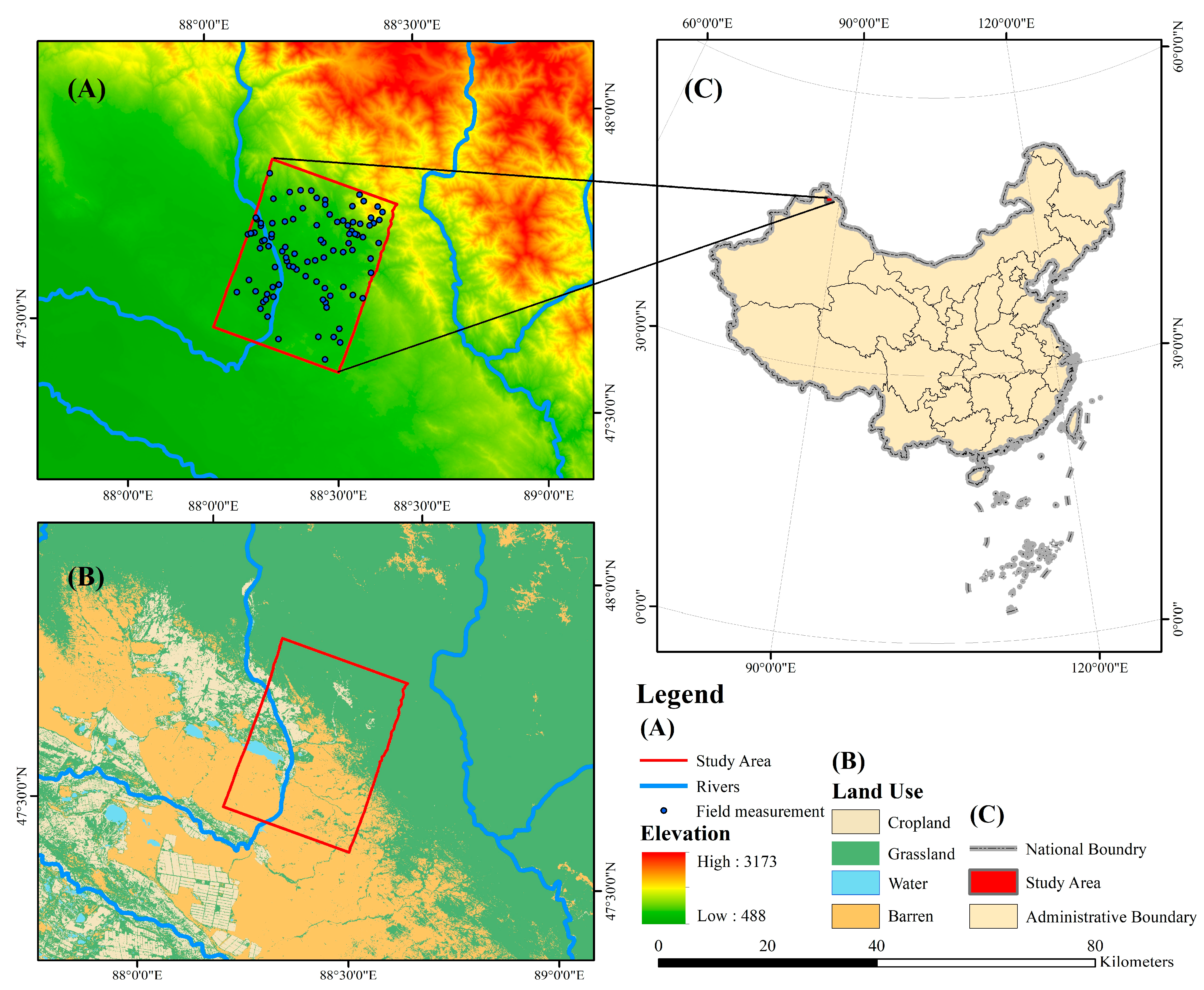
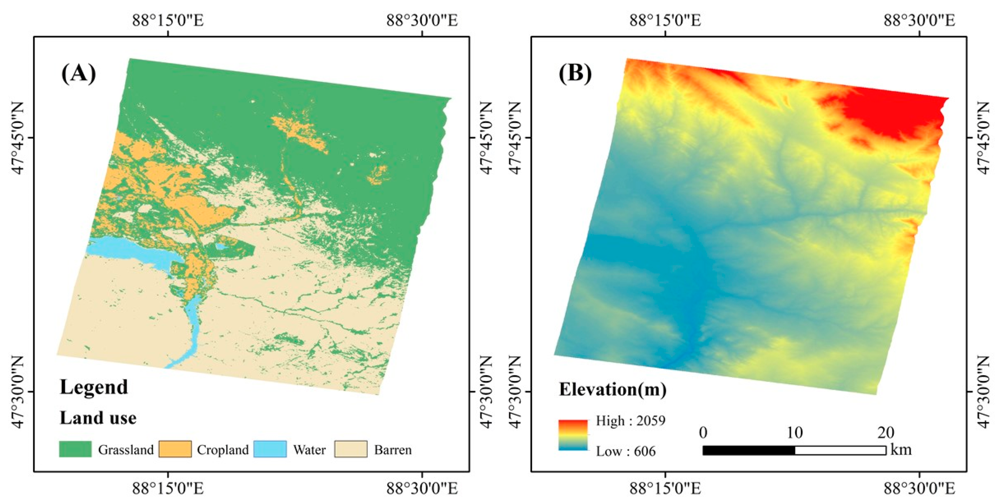
2.1. Overview of the Study Area

The study area (47°49’41.488”–47°29’47.980”N, 88°8’8.016”–88°32’29.168”E) is located in the middle reaches of the Kelan River Basin in Altay region, Xinjiang, China, as shown in Figure 1. Xinjiang, located in the hinterland of Eurasia and northwest China, is a semi-arid region that is highly sensitive to climate change. The region is characterized by a continental climate and extensive internal flow basins, which are entirely dependent on water from the surrounding mountains [36]. More than 80% of the surface runoff in Xinjiang comes from mountainous areas, and snow and ice meltwater account for more than 45% [37]. The northern Xinjiang region is one of the areas with frequent snowmelt flood disasters in Xinjiang. Against the backdrop of a warmer and wetter climate in northwest China, the hydrological processes of the basin have an obvious response to climate change. The main result is the increase in snow cover, leading to the advance of the flood season [38,39]. Therefore, the study of the physical parameters for snow cover in Xinjiang is not only a key indicator for understanding climate change and improving the assessment and utilization efficiency of regional water resources, but also provides more accurate suggestions for flood prevention and disaster prevention.

The water source of the region mainly depends on the supply of snowmelt runoff in the basin [36]. Kelan River is a tributary of the Irtysh River with a total length of 265 km and is mainly supplied by snow meltwater, rainfall water, and groundwater. Among them, snowmelt runoff contributes the most to the river, accounting for about 45% on average. The Kelan River basin has good snow research conditions. The snowfall period in the high mountain area is in early September, while in the plains area, it is in early and middle September, and it melts in the April of the following year [37]. At the same time, the Altay Meteorological Station located along the foothills has abundant snow measurement data, which can provide support for high-resolution snow research. The terrain of the study area gradually flattens from north to south. The northern region is mountainous, above 800 m. The central region is relatively flat, with an altitude of 700–800 m. The lowest altitude is about 600 m in the southwest, and the terrain in the northeast is relatively fragmented. According to the statistics on land use data (Figure 1), the types of land use in the study area in the order from most to least used are grasslands (48.86%), barren lands (41.79%), cropland (7.00%), and bodies of water (2.35%). The distribution among the categories is relatively regular.

2.2. GF-3 Image Data

According to the requirements of C-band SAR images by the EQeau model in autumn and winter, the SAR images of GF-3 in autumn and winter were obtained as the input data of the model. The GF-3 satellite is equipped with a C-band multi-polarization synthetic aperture radar, which was launched on 10 August 2016. It is capable of all-weather operations and can penetrate clouds, vegetation, sand layers, ice, and snow [35]. With a maximum spatial resolution of one meter, GF-3 is currently the SAR satellite with the most imaging modes, including twelve imaging modes such as strip imaging, scanning imaging, and cluster imaging [40]. The third GF-3 satellite was launched on 7 April 2022. Currently, the three GF-3 satellites are evenly distributed on the same orbital plane, and each satellite takes 99 min to orbit the Earth. The maximum revisit period for global observations has been shortened from 84 hours per satellite to twelve hours per satellite, and the average revisit period has been shortened from twelve hours per satellite to 4.8 h per satellite. The same region can be revisited at least two times per day and five times per day on average, and high dynamic imaging can be carried out in the global region. Therefore, GF-3 has the advantages of all-weather detection, high spatial resolution, high temporal resolution, etc. At present, the satellite is rarely applied to snow research. Users can log onto the GF-3 image resources satellite data distribution platform at the Center for Inquiry and Order (http://36.112.130.153:7777/DSSPlatform/index.html (accessed on 28 February 2022)). In this paper, two 1-A-level GF-3 images are used to achieve high-resolution SWE inversion based on the GF-3 through model optimization. The image parameters used in this paper are shown in

Table 1. The Gf-3 image information.

Date	Imaging Mode	Polarization	Pixel Size/m	Incidence Angle (°)	Longitude of the Center Point (°)	Latitude of the Center Point (°)
2022/2/28	QPSI	HH/HV/VV/VH	2.25×5.54	35.99	88.375952	47.652896
2021/11/04	QPSI	HH/HV/VV/VH	2.25×5.54	35.99	88.297601	47.672924

. The spatial resolution of the two images is 8 m. This paper uses the overlapping area of the two images as the research area to carry out research and analysis (Figure 1).

2.3. Field Measurement Data

Data input, parameter optimization, and accuracy verification of the EQeau model requires access to information on field parameters such as snow depth, snow density, snow water equivalent, and underlying conditions for the same period as the images. The synchronous measurement experiment on snow cover was carried out in the study area from 25 February to 1 March 2022. During the measurement period, there was no rainfall or snowfall in the study area, the weather was stable with no significant temperature or strong wind, and the maximum temperature was kept below 0 °C. Therefore, it was considered that the snow surface condition had not changed significantly. The distribution of measurement points is shown in Figure 1.

The main measurement parameters are snow density, snow depth, and the SWE. The main instruments used are a snow bucket, ruler, electronic scale, and electronic thermometer. Snow sampling is accomplished by inserting the bucket vertically into the bottom of the snow and lifting it along the bottom. At this point, the total weight and depth of the snow can be recorded. The final data for each measurement site were obtained by finding the average of three suitable points within 20 m. The unit of the SWE is g/cm² or kg/m². Thus far, the snow depth, snow density, and SWE values of all measurement points are obtained as the optimization input parameters a model’s optimization input parameters and verification parameters the measurement points is shown in

Table 2. General situation of snow cover parameters at measurement points.

Number of Measurement Points	Minimum Snow Density (kg/m3)	Maximum Snow Density (kg/m3)	Average Snow Density (kg/m3)	Minimum Snow Depth (m)	Maximum Snow Depth (m)	Average Snow Depth (m)
93	138	245	187	0.107	0.43	0.249

.

2.4. Other Data

In addition to GF-3 remote sensing image and field measured data, the digital elevation model (DEM) and land use coverage are also needed in this paper to achieve the further detailed division of the study area. The DEM used was ASTER GDEM 30 m data (obtained at https://www.gscloud.cn/ (accessed on 10 January 2022)). Therefore, Yang et al.’s annual land cover data set in China based on Landsat-8 were selected [41]. The resolution of this dataset is 30 m, and the data are obtained from remote sensing images with a long time series and high precision. The topography and land use in the study area are shown in Figure 1.

3. Methodology

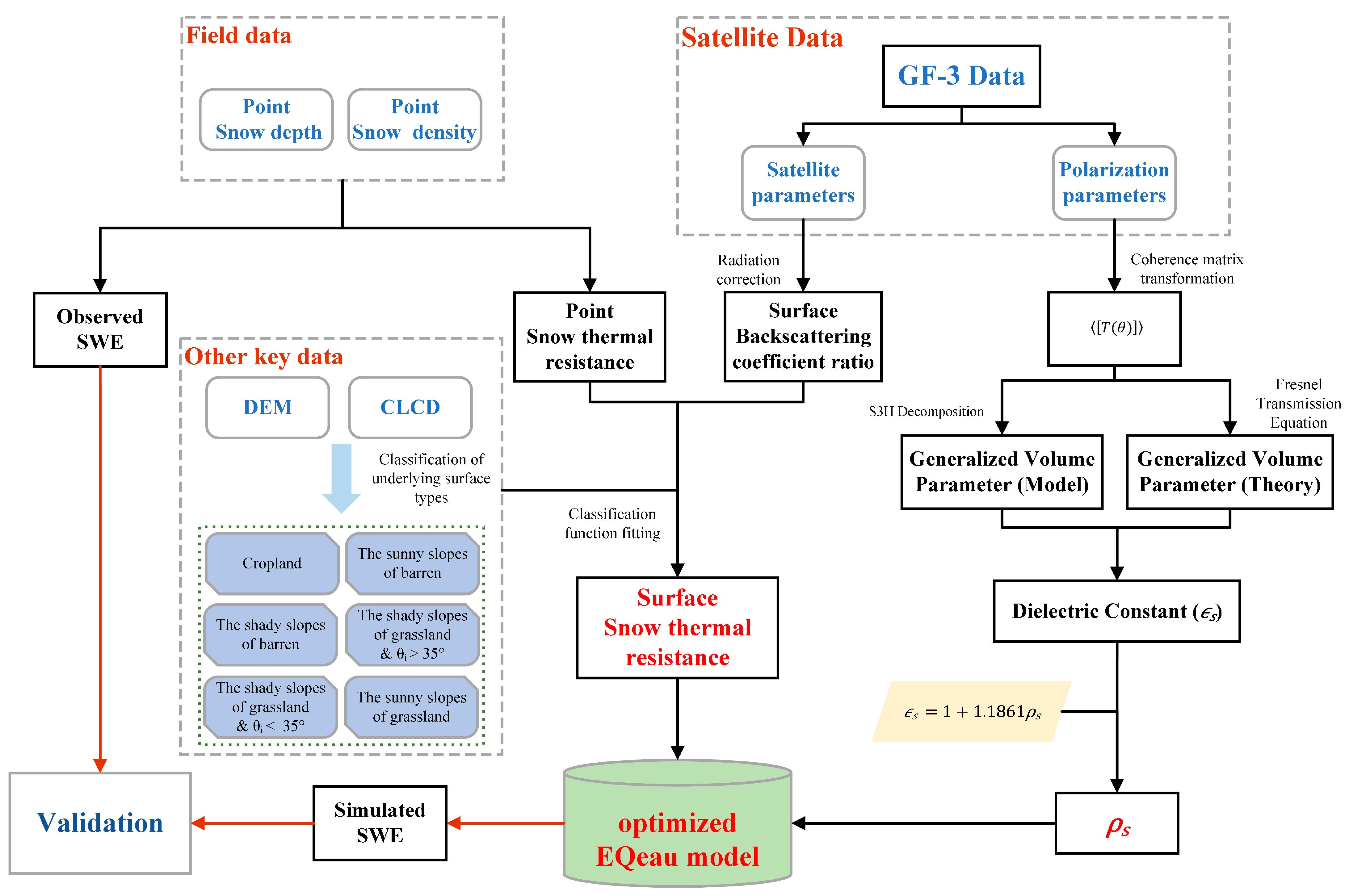
3.1. Research Design

In this paper, the EQeau SWE inversion model is improved based on an advanced GF-3 SAR satellite’s fully polarized images, combined with field observations of the study area in the same period, the S3H decomposition method, and the land classification of the study area. The research route is shown in Figure 2, which refers to the work of Singh et al. [18] and mainly includes the steps described below.

Step 1: The GF-3 image was preprocessed to calculate the ratio of backscattering coefficients.

Step 2: Combined with radar parameters and surface parameters, the semi-empirical formula of the backscattering coefficient ratio and snow thermal resistance was obtained according to the results of the ground classification, and the model influence of the constrained backscattering coefficient ratio was realized.

Step 3: The S3H decomposition was used to invert the snow density in the study area to reduce the impact of the snow density error on the model’s accuracy.

Step 4: The SWE of the study area was calculated according to the optimized semi-empirical formula, and the EQeau model was improved.

3.2. EQeau Model

The EQeau model was first proposed in 1998 and was applied by Bernier et al. to invert the SWE model of the Eton River Basin in Canada [27]. The EQeau model uses snow thermal resistance instead of snow depth as the input parameter of the snow water equivalent via an empirical formula. Meanwhile, the model is based on the correlation between the snow thermal resistance and backscatter coefficient ratio and is used jointly with C-band SAR images to obtain snow thermal resistance values in the study area. Moreover, the snow water equivalent is calculated by combining the spatial interpolation results of the observed snow density values. The principle of this model is as follows:

Firstly, the model expression is established according to the empirical formula. In general, the snow water equivalent is calculated by the product of the snow depth and the snow density.

$$SWE=D_S\times {\rho }_S$$

(1)

where $SWE$ represents the snow water equivalent (kg/m²), $D_S$ represents snow depth (m), and ${\rho }_S$ represents snow density (kg/m³).

At the same time, snow thermal resistance is the ratio of snow depth to snow thermal conductivity, which is an index characterizing snow’s ability to hinder heat conduction.

$$R_S=\frac{D_S}{K_S}$$

(2)

where $R_S$ represents the thermal resistance of snow cover (m² × k/w) and $K_S$ represents snow thermal conductivity. According to Raudviki ‘s research results [42], snow thermal conductivity is a function of snow density, as shown in Formula (3):

$$K_S=A{\rho }_S^2+B{\rho }_S+C$$

(3)

where A = 2.83056 × 10⁻⁶, B = −9.09947 × 10⁻⁵, and C = 3.19739 × 10⁻². Thus, the calculation formula of the SWE can be transformed into Formula (4).

$$SWE=K_S\times {\rho }_S\times R_S=\left(A{\rho }_S^3+B{\rho }_S^2+C{\rho }_S\right)\times R_S$$

(4)

The second step is to obtain the snow density in the study area. According to the EQeau model, researchers usually use the spatial interpolation method of the observation points to obtain the snow density in the study area. The spatial interpolation method is a spatial statistical method employed to obtain the overall values of the study area based on the values and spatial relationships of the observation points.

The third step is to explore the relationship between the backward scattering coefficient ratio and the thermal resistance of snow accumulation in the study area using parameter fitting. According to the conclusions of Bernier et al., parameter fitting can be carried out between the backscattering coefficient ratio of the C-band SAR image and the snow thermal resistance. It is usually expressed in logarithmic form, as shown in Formula (5).

$$BR=f\left(R_S\right)=a_1\times \ln \left(R_S\right)+b_1$$

(5)

where $BR$ is the backscattering coefficient ratio.

Therefore, by establishing an empirical formula, the snow thermal resistance is replaced by the backscattering coefficient ratio, as shown in Formula (6), to achieve the purpose of using SAR to extract the snow water equivalent.

$$SWE=\left(A{\rho }_S^3+B{\rho }_S^2+C{\rho }_S\right)\times \left(a_2\ast e^{b_2\times BR}\right)$$

(6)

Chokmani et al. analyzed the EQeau model in 2006 and found that the main factors affecting the model lie in two areas [31]: the results of the spatial interpolation of snow density and the results of the fitting of the backward scattering coefficient ratio to the snow thermal resistance. To improve the accuracy of the model, it is necessary to also improve the accuracy of these two components.

3.3. Optimization of the Model

3.3.1. Classification of Underlying Surface Types

According to the existing research conclusions [27,43], the influence of the backscattering coefficient ratio on the model mainly comes from the soil roughness, soil moisture, radar polarization mode, and local incidence angle, and these factors make the fit of the snow thermal resistance to the backscattering coefficient ratio decrease and affects the model’s accuracy. The backscattering coefficient ratio is inversely related to the soil roughness and soil moisture, and positively related to the local incidence angle. Additionally, the backscattering coefficient ratio is influenced by the radar polarization mode. When the local incidence angle is not fixed, the polarization mode has more influence. However, the co-polarization mode can suppress the effect of the local incidence angle on the backscattering coefficient ratio in winter and autumn and is the model’s optimal polarization mode.

Since the land use types in the study area are not the same, the topography is undulating and the specific values of soil moisture and soil roughness in the study area are missing, it is not possible to achieve quantitative constraints on the influence of these factors on the backscattering coefficient ratio. Therefore, it is necessary to optimize the fit between the snow thermal resistance and the backscattering coefficient ratio in winter and autumn by optimizing the model’s parameters to suppress the influence of the polarization mode and other effects for the specific topography and land use type conditions in the study area. According to existing studies, it has been shown that there is a relationship between soil roughness, soil moisture, and underlying surface type. The distribution of surface roughness and soil moisture is more concentrated in the same underlying surface type [44,45,46,47]. Therefore, adding the type of underlying surface to the model as a constraint condition can reduce the influence of external factors on the backscattering coefficient to improve the fitting accuracy. As shown in Figure 1B, the main underlying surface types in the study area include cropland, grassland and barren. Meanwhile, there is a large difference in the amount of solar radiation received on the sunny and shady slopes, which leads to a large difference in soil moisture. Therefore, the digital elevation model was used to extract the shady slope and sunny slopes for further classification. According to the conclusion of Wang et al., using the satellite incidence angle as the dividing boundary can effectively reduce the influence of local incidence angle on the fitting [29]. Finally, according to the type of underlying surface in the study area, the incident angle, shady slopes, and sunny slopes are introduced into each category for further division. Because the cropland is located on sunny slopes, and the local incidence angle is smaller the than incidence angle, it is not further divided. The research area was finally divided into six categories; the specific categories are shown in

Table 3. Classification of land classes and number of observation points.

Land Category	Number of Fitting Samples	Number of Validation Samples	Total Number
Cropland	12	3	15
The shady slopes of barren	12	3	15
The sunny slopes of barren	12	2	14
$\mathrm{The}\mathrm{shady}\mathrm{slopes}\mathrm{of}\mathrm{grassland}\&{\theta }_i$$>{35}^{°}$	6	2	8
$\mathrm{The}\mathrm{shady}\mathrm{slopes}\mathrm{of}\mathrm{grassland}\&{\theta }_i$$<{35}^{°}$	19	5	24
The sunny slopes of grassland	13	4	17

.

3.3.2. Singh–Cloude Three-Component Hybrid Decomposition (S3H Decomposition)

In previous studies of SWE inversion based on the EQeau model, the input of snow density was usually the average value of the measured data or spatial interpolation, which could not effectively describe the variation in the snow density in the study area. Other methods using SAR images to extract snow density, such as the co-polarized phase difference (CPD) method [48], have higher requirements on SAR images, which require two overlapping images as a reference. Thus, the method is less applicable. Singh–Cloude three-component hybrid (S3H) decomposition is a fully polarized SAR image decomposition method proposed by Singh et al. in 2017. S3H decomposition is a modification of Cloude’s three-component mixed decomposition scheme [49]. It uses a rotating 3 × 3 coherence matrix [T] to rotate the orientation angle of the solution around the line of sight [50] and implements an extended volume scattering model. The principle of this method is mainly to use the volume scattering parameter obtained after the polarization decomposition and the Fresnel transmission coefficient to establish an equation to estimate for the dielectric constant of the snowpack. The snow density is then found by the empirical relationship between the dielectric constant of the snowpack and snow density. The volume scattering parameters obtained through decomposition have been used in snow density inversion research in many places, and good results have been achieved [18,51].

In the existing S3H extended decomposition method, the spherical shape of snow particles is taken into account to accurately express the volume scattering model [18]. The results of S3H decomposition mainly include surface scattering, double projectile scattering, and the volume scattering power coefficient, while on the surface adjacent to snow cover, double projectile scattering has little influence and can be ignored [52]. S3H is decomposed as follows:

$$\begin{gathered} \langle \left[T\left(\theta \right)\right]\rangle =m_v\left[\begin{array}{ccc}{\left|\gamma \right|}^2& 0& 0\\ 0& \frac{1}{2}& 0\\ 0& 0& \frac{1}{2}\end{array}\right]+ \\ \left[\begin{array}{ccc}{m}_s{\cos }^2\alpha +m_d{\sin }^2\alpha & \cos \alpha \sin \alpha e^{j\varnothing }\left(m_d-m_s\right)& 0\\ \cos \alpha \sin \alpha e^{-j\varnothing }\left(m_d-m_s\right)& m_d{\cos }^2\alpha +m_s{\sin }^2\alpha & 0\\ 0& 0& 0\end{array}\right] \end{gathered}$$

(7)

where $m_s$, $m_d$ and $m_v$ are the surface scattering, double-bounce scattering, and volume scattering power coefficient, respectively. The data we selected are GF-3 polarization data, which can be transformed into polarization coherence matrix T(θ). ${\left|\gamma \right|}^2$ is the generalized volume scattering parameter. This method applies the orthogonality principle of surface and dihedral angular components. The orthogonality condition is expressed as ${\alpha }_d+{\alpha }_s=\frac{\pi }{2}$, ${\varnothing }_d-{\varnothing }_s=\pm \pi$ [52]. ${\varnothing }_d$ and ${\varnothing }_s$ are the scattering phases of surface and double bounce scattering, respectively. Through orthogonality conditions, the two are combined into $\varnothing$ in Formula (7).

Moreover, since a large number of randomly distributed snow particles can be used as Rayleigh scattering objects, the average volume scattering coherence matrix can be expressed as the integral of the volume scattering coherence matrix of randomly distributed spherical particles in a resolution unit at all possible angles $\theta$:

$$\langle {\left[\mathrm{T}\left(\mathsf{\theta }\right)\right]}_{vol}\rangle ={\displaystyle \int }{\left[\mathrm{T}\left(\mathsf{\theta }\right)\right]}_{vol}P\left(\theta \right)d\theta =\left[\begin{array}{ccc}{\left|\gamma \right|}^2& 0& 0\\ 0& \frac{1}{2}& 0\\ 0& 0& \frac{1}{2}\end{array}\right]$$

(8)

Among them,

$$P\left(\theta \right)=\frac{1}{2\pi };\hspace{1em}0<\theta <2\pi$$

(9)

$${\left|\gamma \right|}^2=\frac{\langle {\left|S_{HH}^{vol}+S_{VV}^{vol}\right|}^2\rangle }{\langle {\left|S_{HH}^{vol}-S_{VV}^{vol}\right|}^2\rangle }=\frac{{\left|{\gamma }_{HH}+{\gamma }_{VV}\right|}^2}{{\left|{\gamma }_{HH}-{\gamma }_{HH}\right|}^2}$$

(10)

${\gamma }_{HH}$ and ${\gamma }_{VV}$ are Fresnel transmission coefficients of the HH and VV polarization of SAR images respectively. According to Fresnel’s transmission equation and Snell’s law, Fresnel’s transmission coefficient is expressed as follows:

$${\gamma }_{HH}=\frac{2\cos {\theta }_i}{\cos {\theta }_i+\sqrt{{ϵ}_s-{\sin }^2{\theta }_i}}$$

(11)

$${\gamma }_{VV}=\frac{2\sqrt{{ϵ}_s}\cos {\theta }_i}{{ϵ}_s\cos {\theta }_i+\sqrt{{ϵ}_s-{\sin }^2{\theta }_i}}$$

(12)

Therefore, when the double-bounce scattering is assumed to be negligible, that is, when $m_d$ in Equation (7) tends toward zero, ${\left|\gamma \right|}^2$ can be written as follows:

$${\left|\gamma \right|}^2=\frac{T_{11}\left(\theta \right)}{2T_{33}\left(\theta \right)}-\frac{{\left|T_{12}\left(\theta \right)\right|}^2}{2T_{33}\left(\theta \right)\left(T_{22}\left(\theta \right)-T_{33}\left(\theta \right)\right)}$$

(13)

where $T_{11}\left(\theta \right)$ denotes the elements of the first row and first column of the $T\left(\theta \right)$ matrix, and so on. Therefore, ${\left|\gamma \right|}^2$ can become the intermediate variable connecting Formula (7), Formula (10), Formula (11), and Formula (12), thus establishing the connection between ${ϵ}_s$ and the decomposition matrix, where ${ϵ}_s$ is the dielectric constant of snow. The dielectric constant of snow can be obtained by solving the above equation. Combined with the above formula, the following formula can be obtained:

$$\begin{gathered} \frac{{ϵ}_s\cos {\theta }_i+\sqrt{{ϵ}_s-{\sin }^2{\theta }_i}+\sqrt{{ϵ}_s}\left(cos{\theta }_i+\sqrt{{ϵ}_s-{\sin }^2{\theta }_i}\right)}{{ϵ}_s\cos {\theta }_i+\sqrt{{ϵ}_s-{\sin }^2{\theta }_i}-\sqrt{{ϵ}_s}\left(cos{\theta }_i+\sqrt{{ϵ}_s-{\sin }^2{\theta }_i}\right)} \\ =\frac{T_{11}\left(\theta \right)}{2T_{33}\left(\theta \right)}-\frac{{\left|T_{12}\left(\theta \right)\right|}^2}{2T_{33}\left(\theta \right)\left(T_{22}\left(\theta \right)-T_{33}\left(\theta \right)\right)} \end{gathered}$$

(14)

The derivation of Equation (14) is that the dielectric constant of the snowpack is an unknown parameter. The dielectric constant of the snowpack derived from Equation (14) is related to the snow density, which is calculated using the existing empirical formula [53]. The relationship between snow density and the dielectric constant of the snowpack is:

$${ϵ}_s=1+1.861\times {\rho }_S$$

(15)

Thus far, the polarization matrix information contained in the fully polarized SAR image can be obtained by the polarization decomposition method, and the snow density distributed in the study area can be obtained by establishing the relationship between the dielectric constant of the snowpack and the polarization scattering matrix. The results in the formula are algebraic calculations of the matrix after the polarization decomposition, we implement the algebraic calculation of the matrix through Matlab software. The snow density obtained by inversion is compared with the observed values and conventional spatial interpolation methods in Section 4.2.

4. Results

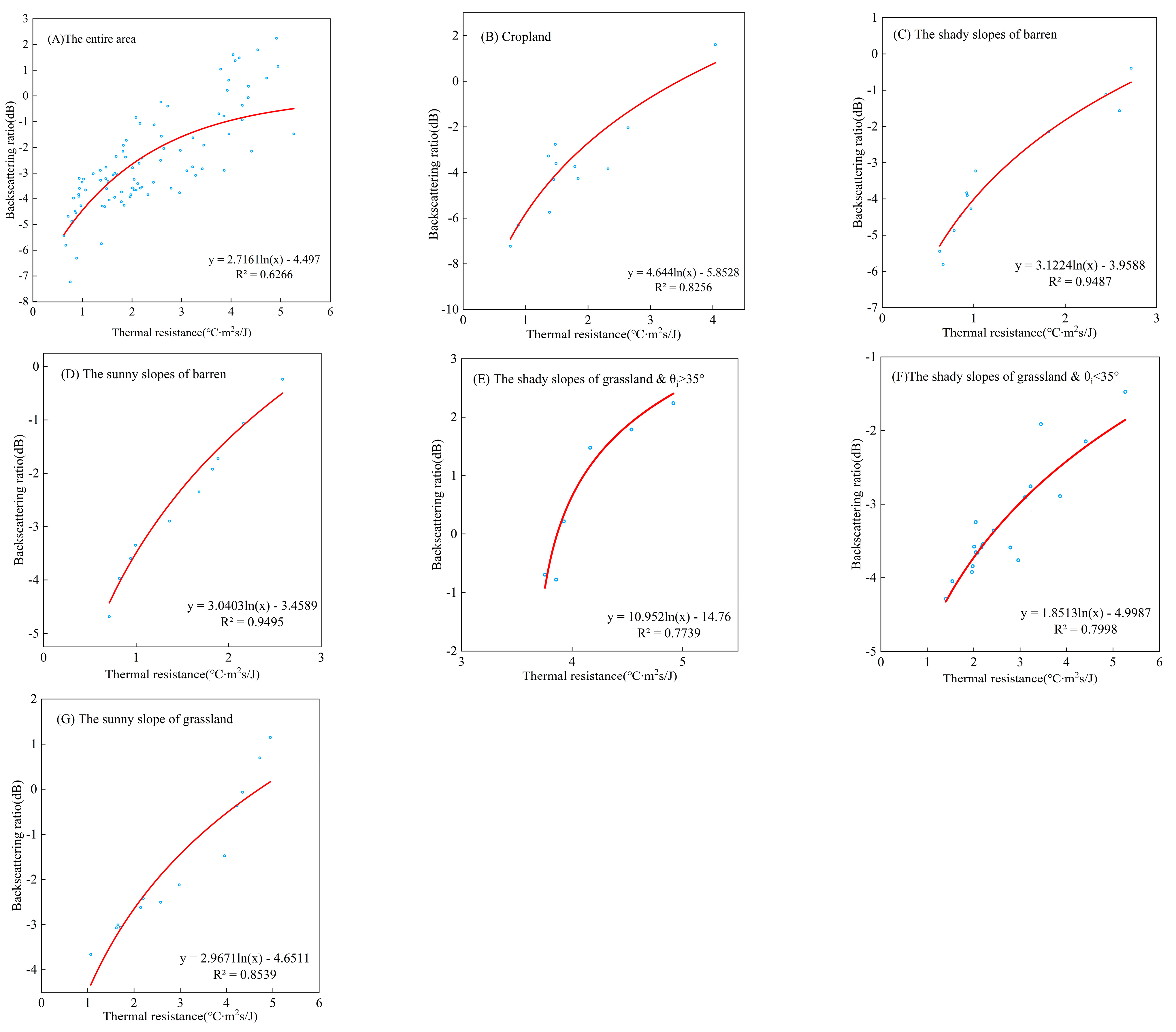
4.1. Optimization of Snow Thermal Resistance Fitting

The EQeau model is a semi-empirical function. As analyzed in Section 3.2, the specific model fitting coefficient will be affected by external conditions. According to the auxiliary data and measured data, the study area is divided into land classes as shown in Table 3, excluding the water areas that are not suitable for the model in the study area. Observation points are divided into different categories according to the land use type of the location for the simulation and verification of different categories. The fitting points in each category accounted for about 80% of the total observation points. To minimize the influence of manual intervention on the experiment, we use random functions to determine the fitting points and verification points in each category. The numbers of fitting points and verification points are shown in Table 3. According to the experience of the EQeau model and the distribution law of measured data in this paper, the logarithmic function was selected as the fitting function to realize the function fitting between the ratio of measured snow thermal resistance and the backscattering coefficient after land classification. The R² value was used to measure the fitting degree between the ratio of the snow thermal resistance and the backscattering coefficient, and the root mean square error was added to measure the deviation between the observed value and the fitted value.

After classifying the study area (Figure 3), the type of snow around the measured values of the thermal resistance and the backward scattering coefficient ratio increased significantly; the unclassified area’s fitting degree, which was lower than 0.62, increased to a fitting degree of over 0.75 in the classified area, including the optimal fitting degree of the bare land types, reaching a function fitting accuracy of more than 90%. It can be seen from the table that the root mean square error between the backscattering coefficient ratio fitted by the snow thermal resistance and the GF-3 inversion value is in the range of 0.195 to 0.722. It means that the fitting degree between the snow thermal resistance and the backscattering coefficient ratio is better after the classification of the study area, which reduces the error caused by the fitting between the two and achieves the purpose of reducing the influence of the backscattering coefficient ratio on the model’s accuracy.

By integrating the fitting relation between the ratio of the snow thermal resistance and the backscattering coefficients in winter and autumn obtained by fitting the above regions, the inverse function was calculated and put into Formula (6), the model coefficients were revised, and finally, a complete EQeau model with optimized parameters suitable for the terrain and underlying surface conditions in the research area was formed. The model coefficients are shown in

Table 4. Comparison of function fitting accuracy and parameters.

Land Category	RMSE (dB)	${\mathit{a}}_2$	${\mathit{b}}_2$
Cropland	0.722	4.644	−5.8528
The shady slopes of barren	0.297	3.1224	−3.9588
The sunny slopes of barren	0.430	3.0403	−3.4589
$\mathrm{The}\mathrm{shady}\mathrm{slopes}\mathrm{of}\mathrm{grassland}\&{\theta }_i$$>{35}^{°}$	0.562	10.952	−14.76
$\mathrm{The}\mathrm{shady}\mathrm{slopes}\mathrm{of}\mathrm{grassland}\&{\theta }_i$$<{35}^{°}$	0.195	1.8513	−4.9987
The sunny slopes of grassland	0.567	2.9671	−4.6511

.

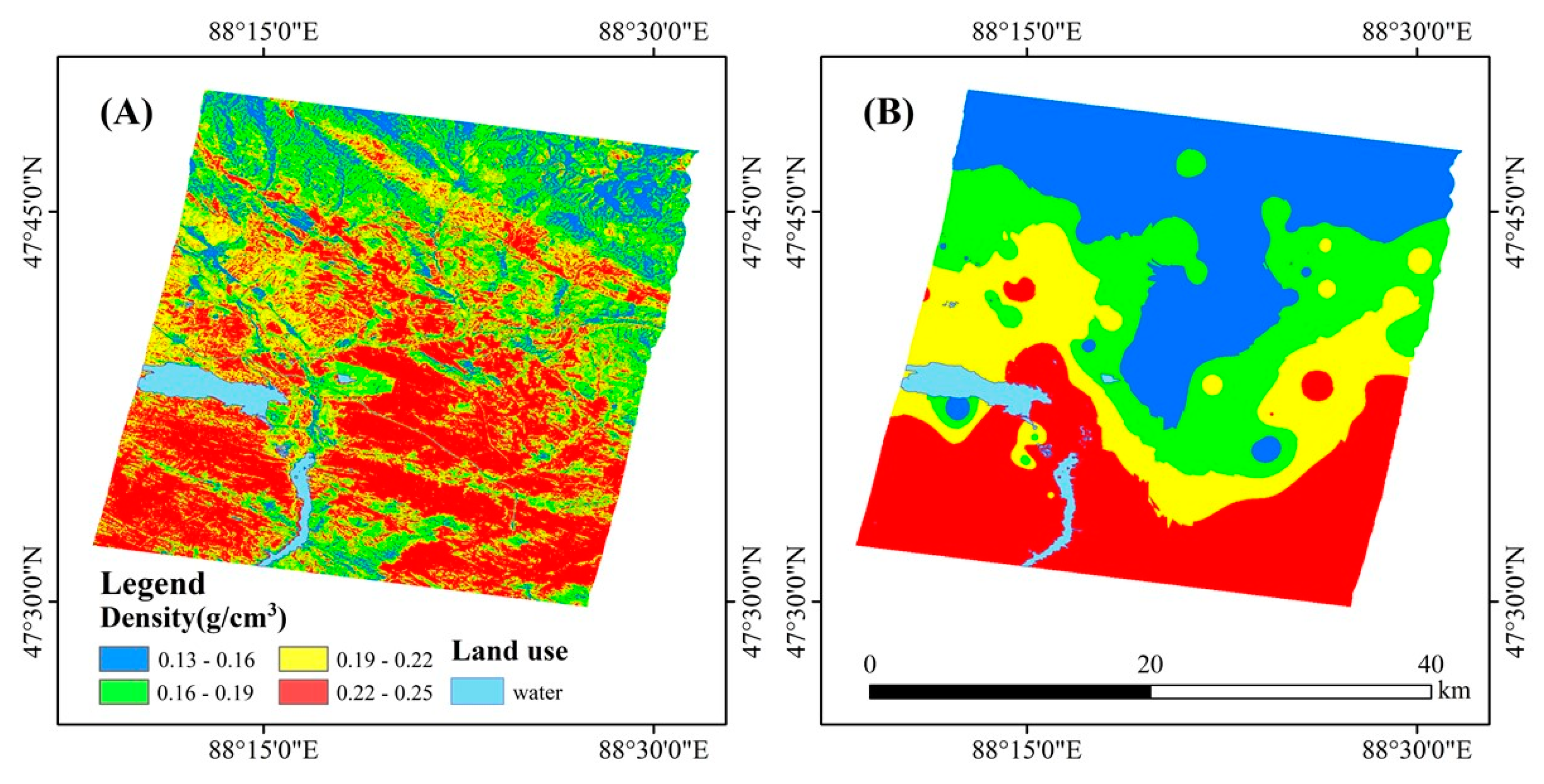
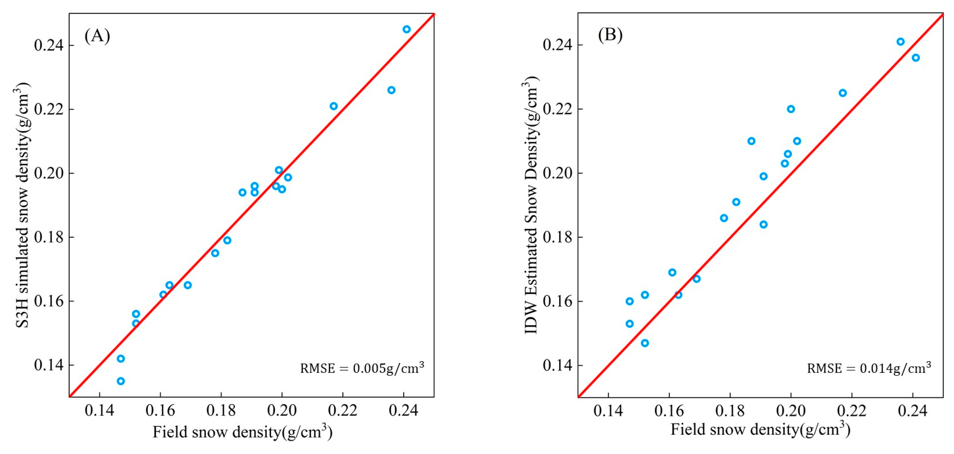
4.2. S3H Decomposition’s Snow Density Extraction Results

S3H decomposition was used to establish the relationship between the snow dielectric constant and volume scattering parameters, and the snow dielectric constant of the snow-covered area in the study area was obtained. The density of snow cover in the study area was calculated according to Formula (15). At the same time, the conventional method was used to carry out spatial interpolation by fitting the measured values of snow density at the observation points. The selected spatial interpolation method is inverse distance weight interpolation, and the test points are reserved for the snow density interpolation test.

As can be seen from the comparison above (Figure 4), the snow density obtained by the two methods is in the range of 0.13 g/cm³ and 0.25 g/cm³. The densities were classified into four classes in the range of 0.03 g/cm³. Superimposed with a topographic map (Figure 5B), it was found that the snow density in the study area decreased gradually along the elevation and from south to north along the latitude, which accords with the law of the snow density measurement in the study area. At the same time, the snow density obtained by S3H decomposition is more refined, and the variation in the snow density at the spatial scale is more obvious, which can better reflect the change in the snow density in the study area.

The snow density value of the verification sample was compared with the results of two types of snow density generation (Figure 6). The RMSE of snow density and the validation sample obtained by S3H decomposition and the IDW spatial interpolation method were 0.005 g/cm³ and 0.014 g/cm³, respectively. The accuracy of the snow density inversion using S3H decomposition was better.

After fitting, it can be found that the snow density obtained by S3H decomposition is closer to the actual value, which may be because compared with the spatial interpolation method, which relies on the measured snow density distributed in different areas, it cannot reflect the spatial variation in the snow density. S3H decomposition can better reflect the spatial distribution of the snow density at a high-resolution scale through the scattering characteristics of the snow body. Therefore, it can be considered that the spatial snow density distribution obtained by S3H decomposition is more accurate, and the snow density map obtained by S3H decomposition inversion can replace the traditional spatial interpolation method of snow density generation to reduce the model error more effectively.

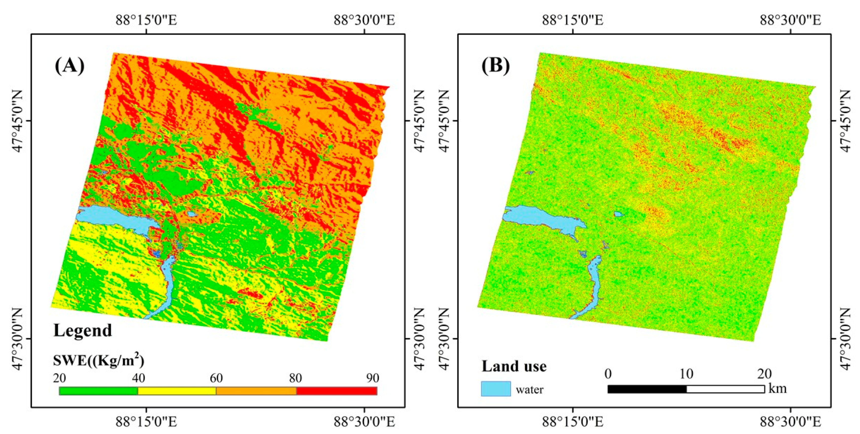
4.3. Results of the Optimized EQeau Model’s Extraction of Snow Water Equivalent

Through the fitting optimization of the snow thermal resistance and the spatial inversion optimization of snow density, the two input parameters of the EQeau model were optimized separately. The thermal resistance fitting values and snow density of different ground snow types were put into Formula (6) to achieve the inversion of the SWE in the study area as a whole. The results are shown in Figure 7.

After the optimization of the model, the overall snow weight in the study area is distributed between 23.7 mm and 87.6 mm, with an average of 48.7 mm. The SWE of the optimized model clearly shows an increasing trend along with the increase in latitude, which is consistent with the trend of the terrain increasing from south to north in the study area (Figure 5A). Among different land types, the SWE of bare land and cultivated land on the sunny slope is the lowest, and the main SWE distribution is 20–40 mm. The SWE obtained from the inversion is relatively high, mainly distributed at 60–90 mm in the grassland with a higher altitude and northern latitude. The performance of the SWE is also different under different constraints of the same underlying surface, which is mainly reflected in the fact that the SWE in shady slope areas is generally higher than in sunny slope areas. This may be because sunshine, wind, and other conditions affect the accumulation of snow on the sunny slope, making the SWE value on the shady slope higher.

At the same time, compared with the results of the model without optimization, the estimation of the SWE between different land types is clearer (Figure 7). The optimized model can clearly distinguish that the snowfall value of the cultivated land in the northern part of the study area is low, but not mixed with the northern grassland. It can be seen that the SWE distribution without optimization is mainly concentrated at 20–60 mm. At the same time, the difference in the SWE between different land types decreases and is difficult to distinguish. This is mainly because the model is not optimized and the fitting degree between the ratio of the snow thermal resistance and the backscattering coefficient is insufficient, which leads to great errors in the simulation of the overall snow thermal resistance value. On the whole, the optimized model can better realize SWE inversion in the study area.

5. Discussion

5.1. Evaluation of Model Accuracy

In the results section, we show the spatial distribution characteristics of snow water equivalents retrieved by the model before and after optimization. In order to verify whether the results obtained by our model are good, it is necessary to compare the model accuracy before and after optimization as well as the accuracy of the optimized model and other methods. We calculated the root mean square error (RMSE), mean absolute error (MAE), and mean relative error (MRE) to compare the original model with the model under different constraints to reflect the difference in accuracy before and after the model’s optimization. The values involved in the accuracy evaluation are randomly selected validation sample points. The specific values are shown in

Table 5. Optimization model inversion accuracy analysis.

Land Category	RMSE (mm)	MAE (mm)	MRE
Overall	5.76	4.89	10.3%
Cropland	6.16	4.77	9.7%
The shady slopes of barren	4.27	3.48	9.3%
The sunny slopes of barren	4.42	3.74	9.2%
$\mathrm{The}\mathrm{shady}\mathrm{slopes}\mathrm{of}\mathrm{grassland}\&{\theta }_i$$>{35}^{°}$	3.76	3.50	6.5%
$\mathrm{The}\mathrm{shady}\mathrm{slopes}\mathrm{of}\mathrm{grassland}\&{\theta }_i$$<{35}^{°}$	7.09	6.38	12.3%
The sunny slopes of grassland	6.18	5.47	11.3%

and

Table 6. Original model inversion accuracy analysis.

Land Category	RMSE (mm)	MAE (mm)	MRE
Overall	12.05	12.89	27.4%
Cropland	12.21	12.21	26.8%
The shady slopes of barren	13.30	12.90	35.0%
The sunny slopes of barren	12.06	11.31	28.0%
$\mathrm{The}\mathrm{shady}\mathrm{slopes}\mathrm{of}\mathrm{grassland}\&{\theta }_i$$>{35}^{°}$	12.81	10.55	18.1%
$\mathrm{The}\mathrm{shady}\mathrm{slopes}\mathrm{of}\mathrm{grassland}\&{\theta }_i$$<{35}^{°}$	17.09	14.61	27.1%
The sunny slopes of grassland	13.69	13.18	16.8%

.

As can be seen from the values in the table, the simulation accuracy of the optimized model is significantly improved in all the local classes. The RMSE distribution of the optimized local classes ranges from 3.76 mm to 7.09 mm. Compared with the model before optimization, the average RMSE decreases by about 6.29 mm, and the estimation accuracy of the SWE is significantly improved. However, the unoptimized EQeau model is not ideal in the study area, with an overall MRE of 27.4%. Although it can still roughly reflect the distribution of the SWE in the study area, the fitting degree between the overall snow thermal resistance and the ratio of the backscattering coefficient decreases due to the lack of constraints, resulting in a wider range of model errors. At the same time, compared with previous studies without snow density process optimization, the overall MRE is 19.5% [54]. In this paper, S3H decomposition was added to optimize snow density, which further improved the model’s accuracy.

At the same time, we present the results of several authors using different methods to invert the snow water equivalent for accuracy comparison (

Table 7. Comparison of snow water equivalent accuracy among different researchers.

Researcher—Time	The Average RMSE (mm)
Patil—2019 [48]	160
Conde—2019 [55]	5.3
Singh—2020 [56]	42.95
Santi—2021 [57]	34.8

). The comparison with other inversions of snow water equivalents using SAR data shows that our results are better in terms of accuracy and have the potential to be applied to basin-scale inversions of snow water equivalents.

Based on the analysis of the results of different researchers above, it can be seen that the inversion of snow water equivalent by remote sensing means will more or less have errors. The error of the model is mainly caused by the error of the measurements and the difference in the mathematical equation of the model in different study areas.

The error of the measurement can be reduced by improving the measurement means, such as using more accurate measuring instruments to measure the snow parameters. The error of the model itself mainly comes from the differences caused by applying the model to different research areas. There are different environment, climate and other conditions in different study areas, which will affect the physical relationship of related snow parameters. Therefore, the application of the improved EQeau model in other regions still needs to consider the environmental conditions of the study area and make corresponding adjustments. In Section 5.3, we will analyze the current limitations of the model and the outlook for the future development of the model.

5.2. Effect of the Number of Fitted Points on the Accuracy of the Model

In this study, measurement data are distributed at all locations in the study area, and the number of observation points also meets the simulation requirements of the model. The fitting between the snow thermal resistance and backscattering coefficient is performed at a ratio of eight to two for the fitting and validation points; however, the model accuracy between the fitting and validation points at different ratios also needs to be discussed in this paper. To avoid overfitting and underfitting, the ratios of 6:4 and 7:3 are chosen for comparison with the results in Table 5, respectively. The values involved in the accuracy evaluation are the validation sample points selected using random selection. The specific values are shown in

Table 8. Different proportions of optimization model accuracy analysis.

Proportion	Land Category	Number of Fitting Samples	Number of Validation Samples	MRE
6:4	Overall	55	38	13.2%
	Cropland	9	6	11.2%
	The shady slopes of barren	9	6	13.4%
	The sunny slopes of barren	9	5	12.6%
	$\mathrm{The}\mathrm{shady}\mathrm{slopes}\mathrm{of}\mathrm{grassland}\&{\theta }_i$$>{35}^{°}$	4	4	9.7%
	$\mathrm{The}\mathrm{shady}\mathrm{slopes}\mathrm{of}\mathrm{grassland}\&{\theta }_i$$<{35}^{°}$	14	10	16.8%
	The sunny slopes of grassland	10	7	15.7%
7:3	Overall	65	28	11.7%
	Cropland	10	5	10.8%
	The shady slopes of barren	10	5	10.6%
	The sunny slopes of barren	10	4	10.3%
	$\mathrm{The}\mathrm{shady}\mathrm{slopes}\mathrm{of}\mathrm{grassland}\&{\theta }_i$$>{35}^{°}$	5	3	8.6%
	$\mathrm{The}\mathrm{shady}\mathrm{slopes}\mathrm{of}\mathrm{grassland}\&{\theta }_i$$<{35}^{°}$	17	7	14.1%
	The sunny slopes of grassland	12	5	12.8%

.

As can be seen from the values in Table 8, the model accuracy will vary with the number of fitting points and verification points. The more fitting points there are, the higher the simulation accuracy of the model. To avoid the insufficient number of verification points caused by increasing the number of fitting points, this paper selects the fitting points and verification points to conduct the test at a ratio of eight to two.

5.3. Uncertainty and Outlook

In this paper, based on the GF-3 SAR data, the EQeau model was optimized to re-alize SWE inversion at the watershed scale, and the results met the needs for practical application. However, it is still difficult to invert snow parameters at the watershed scale due to the difficulty in obtaining field observation data and the limitations of semi-empirical models.

The EQeau model itself has certain limitations. The application of the model should satisfy its basic conditions, the model needs to be applied to shallow snow areas with soil temperatures below 0 °C in winter, and the data used should also be limited to C-band SAR images [27]. EQeau has been used many times around the world. In 2001, Turcotte et al. discussed the method of combining the model with a distributed hydrological model to improve the simulation accuracy of spring snowmelt runoff [58]. In 2006, Chokmani et al. analyzed the uncertainty of the EQeau model in terms of the model coefficients, backscatter coefficient ratio and snow density, and analyzed their influence on the application of the model. At present, this method has been applied in many places in Canada and achieved good results [59]. Corbane et al. used the model in 2005 to retrieve snow water equivalents over the Lebanese plateau [28]. The conclusion proved that the basic conditions of the model should be explored before using it. At the same time, the terrain conditions and field snow observation conditions have a certain impact on the accuracy of the model application. Wang et al. and Zhu et al. applied the model in Xinjiang and northeast China, respectively, and achieved good results [30,54]. Combined with the application of the model by the above scholars, it can be posited that the EQeau model can be used in regions that meet the basic conditions of the model. The application of high-resolution remote sensing images provides conditions for generating high-resolution digital elevation models and land use coverage data. In addition, the GF-3 image includes a full polarization mode, allowing S3H decomposition to also be performed. We believe that the optimized model can be used in locations that meet the preconditions of the EQeau model. However, it needs to be divided according to the topographic features and underlying surface types of specific locations.

With the use of GF-3 satellites, the single-day review of C-band images has become a reality, allowing regional SWE monitoring to occur on a finer time scale. Our study proves that the Gaofen-3 satellite combined with the optimized EQeau model has a good application accuracy. At the same time, because snow-covered areas are mostly mountainous areas in middle and high latitudes, complicated topography and other conditions greatly limit the acquisition of field observation data, as well as the number and spatial distribution of observation points at the watershed scale. At the same time, due to the efficiency of manual work, it is difficult to achieve the synchronous observation of surface data with satellite images. All these factors will influence the final result of the model. Therefore, it is necessary to change the acquisition method of field-measured data to achieve timely, rapid, and accurate parameter observation. At present, with the rise of the Internet of Things and other technologies, some researchers have applied Internet of Things research to regional environmental monitoring. For example, Fang et al. designed an environmental Internet of Things system for environmental parameter monitoring with climate change and ecological monitoring as the theme [60]. Combined with technologies such as the Internet of Things (IoT), this means that more accurate measurements of snow parameters can be obtained through smarter devices. Meanwhile, the application of IoT can realize the measurement of snow parameters at exactly the same time as the satellite imaging so as to reduce the model error caused by the measurement value.

Therefore, we believe that further work is to realize the observation of snow parameters and surface parameters at a finer time scale by combining GF-3 images and the Internet of Things. In addition, the relationship between parameters affecting SWE is further summarized based on observation data for different regions of the model to achieve SWE inversion that is applicable to a larger range of river basins.

6. Conclusions

This paper is based on the advanced C-band SAR imagery GF-3, and referring to the existing research, the EQeau model is optimized to retrieve the high-resolution SWE. The application of GF-3 to basin-scale SWE studies has not been carried out yet, and this paper explores the feasibility of its application to SWE studies by improving the EQeau model. The input parameters of the model are mainly the radar backscatter coefficient ratio and snow density, and the two parts are improved using different methods. Firstly, we combine the actual measurement data of each land class with the land cover of the study area to classify the land classes and achieve the optimization of the fitting of the snow thermal resistance and backscattering coefficient ratio under different land classes. At the same time, the relationship between the snow dielectric constant and the decomposed volume scattering constant is established using the S3H polarization decomposition method to realize the inversion of high-resolution snow density in the study area.

The fitting degree between the snow thermal resistance and the backscattering coefficient ratio can be improved by using land classification. Most of the optimized R² ranges from 0.8 to 0.95, proving that the fitting accuracy has been significantly improved. The volume scattering constant is obtained by S3H decomposition, and the dielectric constant is calculated through integration with Fresnel’s formula. The snow density is calculated by the linear empirical formula of the snow permittivity and snow density. The snow density obtained by S3H decomposition can better reflect the distribution of the snow density in the research area, and the accuracy is higher than that obtained by the traditional spatial interpolation method. The EQeau model using the optimized method has greatly improved the accuracy of the SWE inversion results in the study area, and the total RMSE can reach 5.76 mm, which is consistent with the SWE observation at the watershed scale.

Our study proves that the EQeau model has a good effect when combined with an advanced C-band SAR GF-3 image. Compared with the results before optimization, the MRE decreased from 27.4% to 10.3%. In future studies, the Internet of Things and other advanced technologies should be combined to obtain rapid and timely watershed parameter information and achieve SWE observation in different research demonstration areas.

References

1. Pulliainen, J.; Luojus, K.; Derksen, C.; Mudryk, L.; Lemmetyinen, J.; Salminen, M.; Ikonen, J.; Takala, M.; Cohen, J.; Smolander, T. Patterns and trends of Northern Hemisphere snow mass from 1980 to 2018. Nature 2020, 581, 294–298. [Google Scholar] [CrossRef] [PubMed]
2. Robinson, D.A. Monitoring northern hemisphere snow cover. Glaciol. Data Rep. 1993, 25, 1–25. [Google Scholar]
3. Jonas, T.; Marty, C.; Magnusson, J. Estimating the snow water equivalent from snow depth measurements in the Swiss Alps. J. Hydrol. 2009, 378, 161–167. [Google Scholar] [CrossRef]
4. Kuraś, P.K.; Weiler, M.; Alila, Y. The spatiotemporal variability of runoff generation and groundwater dynamics in a snow-dominated catchment. J. Hydrol. 2008, 352, 50–66. [Google Scholar] [CrossRef]
5. Tanasienko, A.; Yakutina, O.; Chumbaev, A. Effect of snow amount on runoff, soil loss and suspended sediment during periods of snowmelt in southern West Siberia. Catena 2011, 87, 45–51. [Google Scholar] [CrossRef]
6. Zhang, Y.; Ma, N. Spatiotemporal variability of snow cover and snow water equivalent in the last three decades over Eurasia. J. Hydrol. 2018, 559, 238–251. [Google Scholar] [CrossRef]
7. Dozier, J.; Bair, E.H.; Davis, R.E. Estimating the spatial distribution of snow water equivalent in the world’s mountains. Wiley Interdiscip. Rev. Water 2016, 3, 461–474. [Google Scholar] [CrossRef]
8. Schöne, T.; Zech, C.; Unger-Shayesteh, K.; Rudenko, V.; Thoss, H.; Wetzel, H.-U.; Gafurov, A.; Illigner, J.; Zubovich, A. A new permanent multi-parameter monitoring network in Central Asian high mountains–from measurements to data bases. Geosci. Instrum. Methods Data Syst. 2013, 2, 97–111. [Google Scholar] [CrossRef] [Green Version]
9. Fassnacht, S.; Dressler, K.; Bales, R. Snow water equivalent interpolation for the Colorado River Basin from snow telemetry (SNOTEL) data. Water Resour. Res. 2003, 39, 1208. [Google Scholar] [CrossRef] [Green Version]
10. Rice, R.; Bales, R.C.; Painter, T.H.; Dozier, J. Snow water equivalent along elevation gradients in the Merced and Tuolumne River basins of the Sierra Nevada. Water Resour. Res. 2011, 47, W08515. [Google Scholar] [CrossRef] [Green Version]
11. Rittger, K.; Bair, E.H.; Kahl, A.; Dozier, J. Spatial estimates of snow water equivalent from reconstruction. Adv. Water Resour. 2016, 94, 345–363. [Google Scholar] [CrossRef]
12. Serreze, M.C.; Clark, M.P.; Armstrong, R.L.; McGinnis, D.A.; Pulwarty, R.S. Characteristics of the western United States snowpack from snowpack telemetry (SNOTEL) data. Water Resour. Res. 1999, 35, 2145–2160. [Google Scholar] [CrossRef] [Green Version]
13. Romanov, P.; Tarpley, D. Enhanced algorithm for estimating snow depth from geostationary satellites. Remote Sens. Environ. 2007, 108, 97–110. [Google Scholar] [CrossRef]
14. Bair, E.H.; Abreu Calfa, A.; Rittger, K.; Dozier, J. Using machine learning for real-time estimates of snow water equivalent in the watersheds of Afghanistan. Cryosphere 2018, 12, 1579–1594. [Google Scholar] [CrossRef] [Green Version]
15. Jiang, L.; Yang, J.; Zhang, C.; Wu, S.; Li, Z.; Dai, L.; Li, X.; Qiu, Y. Daily snow water equivalent product with SMMR, SSM/I and SSMIS from 1980 to 2020 over China. Big Earth Data 2022, 1–15. [Google Scholar] [CrossRef]
16. Sun, Z.; Shi, J. Development of snow depth and snow water equivalent algorithm in Western China using passive microwave remote sensing data. Adv. Earth Sci. 2006, 21, 1363. [Google Scholar]
17. Chang, A.T.; Foster, J.L.; Hall, D.K. Nimbus-7 SMMR derived global snow cover parameters. Ann. Glaciol. 1987, 9, 39–44. [Google Scholar] [CrossRef] [Green Version]
18. Singh, G.; Verma, A.; Kumar, S.; Ganju, A.; Yamaguchi, Y.; Kulkarni, A.V. Snowpack density retrieval using fully polarimetric TerraSAR-X data in the Himalayas. IEEE Trans. Geosci. Remote Sens. 2017, 55, 6320–6329. [Google Scholar] [CrossRef]
19. Shi, J. Estimation of snow water equivalence with two Ku-band dual polarization radar. In Proceedings of the IGARSS 2004 IEEE International Geoscience and Remote Sensing Symposium, Anchorage, AK, USA, 20–24 September 2004; pp. 1649–1652. [Google Scholar]
20. Shi, J. Snow water equivalence retrieval using X and Ku band dual-polarization radar. In Proceedings of the 2006 IEEE International Symposium on Geoscience and Remote Sensing, Denver, CO, USA, 31 July–4 August 2006; pp. 2183–2185. [Google Scholar]
21. Shi, J.; Dozier, J. Estimation of snow water equivalence using SIR-C/X-SAR. I. Inferring snow density and subsurface properties. IEEE Trans. Geosci. Remote Sens. 2000, 38, 2465–2474. [Google Scholar]
22. Largeron, C.; Dumont, M.; Morin, S.; Boone, A.; Lafaysse, M.; Metref, S.; Cosme, E.; Jonas, T.; Winstral, A.; Margulis, S.A. Toward Snow Cover Estimation in Mountainous Areas Using Modern Data Assimilation Methods: A Review. Front. Earth Sci. 2020, 8, 325. [Google Scholar] [CrossRef]
23. Massonnet, D.; Feigl, K.L. Radar interferometry and its application to changes in the Earth’s surface. Rev. Geophys. 1998, 36, 441–500. [Google Scholar] [CrossRef] [Green Version]
24. Dagurov, P.; Chimitdorzhiev, T.; Dmitriev, A.; Dobrynin, S. Estimation of snow water equivalent from L-band radar interferometry: Simulation and experiment. Int. J. Remote Sens. 2020, 41, 9328–9359. [Google Scholar] [CrossRef]
25. Deeb, E.J.; Forster, R.R.; Kane, D.L. Monitoring snowpack evolution using interferometric synthetic aperture radar on the North Slope of Alaska, USA. Int. J. Remote Sens. 2011, 32, 3985–4003. [Google Scholar] [CrossRef]
26. Leinss, S.; Wiesmann, A.; Lemmetyinen, J.; Hajnsek, I. Snow water equivalent of dry snow measured by differential interferometry. IEEE J. Sel. Top. Appl. Earth Obs. Remote Sens. 2015, 8, 3773–3790. [Google Scholar] [CrossRef] [Green Version]
27. Bernier, M.; Fortin, J.P.; Gauthier, Y.; Gauthier, R.; Roy, R.; Vincent, P. Determination of snow water equivalent using RADARSAT SAR data in eastern Canada. Hydrol. Processes 1999, 13, 3041–3051. [Google Scholar] [CrossRef]
28. Corbane, C.; Somma, J.; Bernier, M.; Fortin, J.; Gauthier, Y.; Dedieu, J. Estimation de L’équivalent en Eau du Couvert Nival en Montagne Libanaise à Partir des Images RADARSAT-1/Estimation of Water Equivalent of the Snow Cover in Lebanese Mountains by Means of RADARSAT-1 Images. Hydrol. Sci. J. 2005, 50, 370. [Google Scholar] [CrossRef]
29. Wang, Z.; Feng, X.; Xiao, P.; He, G. Retrieval of snow water equivalence using SAR data for mountainous area. J. Nanjing Univ. (Nat. Sci.) 2015, 51, 996–1004. [Google Scholar]
30. Zhu, X.; Gu, L.; Ren, R.; He, F. Snow water equivalent retrieval algorithm in Jilin Province of China based on multi-temporal Sentinel-1 data. In Proceedings of the Earth Observing Systems XXIV, San Diego, CA, USA, 9 September 2019; pp. 510–518. [Google Scholar]
31. Chokmani, K.; Bernier, M.; Gauthier, Y. Uncertainty analysis of EQeau, a remote sensing based model for snow water equivalent estimation. Int. J. Remote Sens. 2006, 27, 4337–4346. [Google Scholar] [CrossRef]
32. Morena, L.; James, K.; Beck, J. An introduction to the RADARSAT-2 mission. Can. J. Remote Sens. 2004, 30, 221–234. [Google Scholar] [CrossRef]
33. Torres, R.; Snoeij, P.; Geudtner, D.; Bibby, D.; Davidson, M.; Attema, E.; Potin, P.; Rommen, B.; Floury, N.; Brown, M. GMES Sentinel-1 mission. Remote Sens. Environ. 2012, 120, 9–24. [Google Scholar] [CrossRef]
34. Zhen, L.; Bangsen, T.; Ping, Z.; Changjun, Z.; Guangde, S.; Chang, L. Overview of the snow parameters inversion from synthetic aperture radar. Nanjing Xinxi Gongcheng Daxue Xuebao 2020, 12, 159–169. [Google Scholar]
35. Chen, L.; Letu, H.; Fan, M.; Shang, H.; Tao, J.; Wu, L.; Zhang, Y.; Yu, C.; Gu, J.; Zhang, N. An Introduction to the Chinese High-Resolution Earth Observation System: Gaofen-1~ 7 Civilian Satellites. J. Remote Sens. 2022, 2022, 9769536. [Google Scholar] [CrossRef]
36. Shen, Y.; Wang, G.; Su, H.-C.; Han, P.; Gao, Q.-Z.; Wang, S.-D. Hydrological processes responding to climate warming in the upper reaches of Kelan River Basin with snow-dominated of the Altay Mountains region, Xinjiang. J. Glaciol. Geocryol. 2007, 29, 845–854. [Google Scholar]
37. Qiu-Xiang, W. The changing tendency on the depth and days of snow cover in northern Xinjiang. Adv. Clim. Change Res. 2009, 5, 39. [Google Scholar]
38. Shen, Y.; Su, H.; Wang, G.; Mao, W.; Wang, S.; Han, P.; Wang, N.; Li, Z. The Responses of Glaciers and Snow Cover to Climate Change in Xinjiang (II): Hazards Effects. J. Glaciol. Geocryol. 2013, 35, 1355–1370. [Google Scholar]
39. He, B.; Wang, G.; Su, H.; Shen, Y. Response of Extreme Hydrological Events to Climate Change in the Regions of Altay Mountains, Xinjiang. J. Glaciol. Geocryol. 2012, 34, 927–933. [Google Scholar]
40. Chang, Y.; Li, P.; Yang, J.; Zhao, J.; Zhao, L.; Shi, L. Polarimetric calibration and quality assessment of the GF-3 satellite images. Sensors 2018, 18, 403. [Google Scholar] [CrossRef] [Green Version]
41. Yang, J.; Huang, X. The 30 m annual land cover dataset and its dynamics in China from 1990 to 2019. Earth Syst. Sci. Data 2021, 13, 3907–3925. [Google Scholar] [CrossRef]
42. Raudkivi, A.J. Hydrology: An Advanced Introduction to Hydrological Processes and Modelling; Elsevier: Amsterdam, The Netherlands, 2013. [Google Scholar]
43. Topp, G.C.; Davis, J.; Annan, A.P. Electromagnetic determination of soil water content: Measurements in coaxial transmission lines. Water Resour. Res. 1980, 16, 574–582. [Google Scholar] [CrossRef]
44. Tao, H.; Chen, Q.; Li, Z.; Zeng, J.; Chen, X. Improvement of soil surface roughness measurement accuracy by close-range photogrammetry. Trans. Chin. Soc. Agric. Eng. 2017, 33, 162–167. [Google Scholar]
45. Li, X.; Cai, X.; Song, Y. Research of the distribution of national scale surface roughness length with high resolution in China. Plateau Meteorol. 2014, 33, 474–482. [Google Scholar]
46. Western, A.W.; Grayson, R.B.; Blöschl, G.; Willgoose, G.R.; McMahon, T.A. Observed spatial organization of soil moisture and its relation to terrain indices. Water Resour. Res. 1999, 35, 797–810. [Google Scholar] [CrossRef] [Green Version]
47. Gómez-Plaza, A.; Martınez-Mena, M.; Albaladejo, J.; Castillo, V. Factors regulating spatial distribution of soil water content in small semiarid catchments. J. Hydrol. 2001, 253, 211–226. [Google Scholar] [CrossRef]
48. Patil, A.; Singh, G.; Rüdiger, C. A novel approach for the retrieval of snow water equivalent using SAR data. In Proceedings of the IGARSS 2019-2019 IEEE International Geoscience and Remote Sensing Symposium, Yokohama, Japan, 28 July–2 August 2019; pp. 3233–3236. [Google Scholar]
49. Cloude, S. Polarisation: Applications in Remote Sensing; OUP Oxford: Oxford, UK, 2009. [Google Scholar]
50. Yamaguchi, Y.; Sato, A.; Boerner, W.-M.; Sato, R.; Yamada, H. Four-component scattering power decomposition with rotation of coherency matrix. IEEE Trans. Geosci. Remote Sens. 2011, 49, 2251–2258. [Google Scholar] [CrossRef]
51. Varade, D.; Manickam, S.; Dikshit, O.; Singh, G. Modelling of early winter snow density using fully polarimetric C-band SAR data in the Indian Himalayas. Remote Sens. Environ. 2020, 240, 111699. [Google Scholar] [CrossRef]
52. Singh, G.; Yamaguchi, Y.; Park, S.-E.; Cui, Y.; Kobayashi, H. Hybrid Freeman/eigenvalue decomposition method with extended volume scattering model. IEEE Geosci. Remote Sens. Lett. 2012, 10, 81–85. [Google Scholar] [CrossRef]
53. Matzler, C. Microwave permittivity of dry snow. IEEE Trans. Geosci. Remote Sens. 1996, 34, 573–581. [Google Scholar] [CrossRef]
54. Wang, Z. Retrieval of Snow Water Equivalence Using SAR Data for Typical Area of Manas River Basin in Xinjiang, China. Ph.D. Dissertation, Nanjing University, Nanjing, China, 2014. [Google Scholar]
55. Conde, V.; Nico, G.; Mateus, P.; Catalão, J.; Kontu, A.; Gritsevich, M. On the estimation of temporal changes of snow water equivalent by spaceborne SAR interferometry: A new application for the Sentinel-1 mission. J. Hydrol. Hydromech. 2019, 1, 93–100. [Google Scholar] [CrossRef] [Green Version]
56. Patil, A.; Singh, G.; Rüdiger, C. Retrieval of snow depth and snow water equivalent using dual polarization SAR data. Remote Sens. 2020, 12, 1183. [Google Scholar] [CrossRef] [Green Version]
57. Santi, E.; Brogioni, M.; Leduc-Leballeur, M.; Macelloni, G.; Montomoli, F.; Pampaloni, P.; Lemmetyinen, J.; Cohen, J.; Rott, H.; Nagler, T. Exploiting the ANN potential in estimating snow depth and snow water equivalent from the airborne SnowSAR data at X-and Ku-bands. IEEE Trans. Geosci. Remote Sens. 2021, 60, 4301216. [Google Scholar] [CrossRef]
58. Turcotte, R.; Fortin, J.-P.; Bernier, M.; Gauthier, Y. Developments for Snowpack Water Equivalent Monitoring Using Radarsat Data as Input to the Hydrotel Hydrological Model; Iahs Publication: Wallingford, UK, 2001; pp. 374–378. [Google Scholar]
59. Gauthier, Y.; Bernier, M.; Fortin, J.-P.; Gauthier, R.; Roy, R.; Vincent, P. Operational Determination of Snow Water Equivalent Using Radarsat Data over a Large Hydroelectric Complex in Eastern Canada; Iahs Publication: Wallingford, UK, 2001; pp. 343–348. [Google Scholar]
60. Fang, S.; Da Xu, L.; Zhu, Y.; Ahati, J.; Pei, H.; Yan, J.; Liu, Z. An integrated system for regional environmental monitoring and management based on internet of things. IEEE Trans. Ind. Inform. 2014, 10, 1596–1605. [Google Scholar] [CrossRef]
Figure 1. (A) shows the topography of the study area and the location of measurement points; (B) shows the land use types in the study area and (C) shows the location of the study area in China.
Remotesensing 14 04931 g001
Figure 2. Flowchart of the optimized SWE inversion model for GF-3.
Remotesensing 14 04931 g002
Figure 3. (A) shows the fit of snow thermal resistance to backscattering coefficient ratio for all unclassified observations; (BG) shows the fit of snow thermal resistance to backscattering coefficient ratio for each class after classification.
Remotesensing 14 04931 g003
Figure 4. S3H polarization decomposition (A) and IDW interpolation (B) inversion snow density results.
Remotesensing 14 04931 g004
Figure 5. Land cover in the study area (A) and study area topography(B).
Remotesensing 14 04931 g005
Figure 6. Distribution of validated sample values and inversion values for S3H decomposition (A) and IDW interpolation (B) of snow density.
Remotesensing 14 04931 g006
Figure 7. Optimized model (A) and original model (B) snow water equivalent inversion results.
Remotesensing 14 04931 g007