Article

An Improved RANSAC Outlier Rejection Method for UAV-Derived Point Cloud

1
Department of Environmental Resources Engineering, College of Environmental Science and Forestry, State University of New York, Syracuse, NY 13210, USA
2
Department of Civil and Architectural Engineering, University of Miami’s Institute for Data Science & Computing, Coral Gables, FL 33146, USA
*
Author to whom correspondence should be addressed.
Remote Sens. 2022, 14(19), 4917; https://doi.org/10.3390/rs14194917
Submission received: 18 August 2022 / Revised: 20 September 2022 / Accepted: 26 September 2022 / Published: 1 October 2022

Abstract

:
A common problem with matching algorithms, in photogrammetry and computer vision, is the imperfection of finding all correct corresponding points, so-called inliers, and, thus, resulting in incorrect or mismatched points, so-called outliers. Many algorithms, including the well-known randomized random sample consensus (RANSAC)-based matching, have been developed focusing on the reduction of outliers. RANSAC-based methods, however, have limitations such as increased false positive rates of outliers, and, consequently resulting in fewer inliers, an unnecessary high number of iterations, and high computational time. Such deficiencies possibly result from the random sampling process, the presence of noise, and incorrect assumptions of the initial values. This paper proposes a modified version of RANSAC-based methods, called Empowered Locally Iterative SAmple Consensus (ELISAC). ELISAC improves RANSAC by utilizing three basic modifications individually or in combination. These three modifications are (a) to increase the stability and number of inliers using two Locally Iterative Least Squares (LILS) loops (Basic LILS and Aggregated-LILS), based on the new inliers in each loop, (b) to improve the convergence rate and consequently reduce the number of iterations using a similarity termination criterion, and (c) to remove any possible outliers at the end of the processing loop and increase the reliability of results using a post-processing procedure. In order to validate our proposed method, a comprehensive experimental analysis has been done on two datasets. The first dataset contains the commonly-used computer vision image pairs on which the state-of-the-art RANSAC-based methods have been evaluated. The second dataset image pairs were captured by a drone over a forested area with various rotations, scales, and baselines (from short to wide). The results show that ELISAC finds more inliers with a faster speed (lower computational time) and lower error (outlier) rates compared to M-estimator SAmple Consensus (MSAC). This makes ELISAC an effective approach for image matching and, consequently, for 3D information extraction of very high and super high-resolution imagery acquired by space-borne, airborne, or UAV sensors. In particular, for applications such as forest 3D modeling and tree height estimations where standard matching algorithms are problematic due to spectral and textural similarity of objects (e.g., trees) on image pairs, ELISAC can significantly outperform the standard matching algorithms.

1. Introduction

Matching is the process of finding the corresponding points in two or more images of the same area (overlapping images) and is a fundamental step in 3D model generation in photogrammetry and computer vision [1]. Matching is used in many photogrammetric and computer vision applications, such as image registration, triangulation, 3D model and digital surface model (DSM) generation, change detection, target detection, and image mosaicking. Despite the presence of many matching algorithms, the accurate, fast, and highly reliable performance of existing matching processes still has significant limitations due to the complex characteristics of the images used in photogrammetric applications, as well as the requirements for improving the accuracy, speed, and reliability of this process [2,3,4,5,6,7,8]. For example, standard matching algorithms such as the well-known Randomize Random SAmple Consensus (RANSAC) do not provide promising results when applied to UAV imagery over forest areas due to spectral and textural similarities of objects, resulting in a fairly large number of mismatched points (outliers or noise).
Matching is a fundamental step in photogrammetry for the generation of DSM using a set of two or more overlapping images. The traditional photogrammetric procedure is effective when applied to imagery acquired by metric cameras (sensors) onboard aerial or space-borne platforms. Although there are UAVs with metric cameras, most of the UAVs on the market capture imagery with nonmetric cameras, resulting in the ineffectiveness of traditional photogrammetry for applications such as DSM generation. In addition, the super high-spatial resolution of UAV images (i.e., centimetric level) makes the use of conventional photogrammetric processing less effective [9,10]. In general, the DSM generation steps are (1) feature extraction and matching; (2) finding the best match (outlier rejection); (3) triangulation, bundle block adjustment, and sparse point cloud generation; (4) point cloud densification; and, finally, (5) DSM generation. The high number of inliers increases the observations and directly improves the accuracy of triangulation, bundle block adjustment, and sparse point cloud. Therefore, finding more inliers (best matches) is essential for generating a denser and well-distributed sparse point cloud and, consequently, a preciser DSM [11,12].
One of the challenges in processing UAV data for 3D generation is the presence of outliers in the matching step and, as a result, the generation of the sparse and dense points cloud with low accuracy and, finally, the generation of DSM of the scene with low accuracy [13]. Therefore, it is necessary to eliminate the outliers in each stage, including the generation of tie, sparse, and dense point clouds, in order to increase the accuracy and quality of the matching process and, consequently, generate an accurate DSM.
In general, the outlier removal methods can be categorized as handcrafted and deep learning methods [14]. There are various traditional (handcrafted) methods for removing outliers, such as M-estimators, L-estimators, R-estimators, Least Median Squares (LMedS), and Hough transform [15]. One of the most widely used algorithms is RANSAC, which estimates both matched features and outliers [16]. RANSAC is based on an iterative selection of minimal random samples in order to estimate the model parameters [16]. To find correct matches, RANSAC needs a high number of iterations to detect the possible inliers among the existing outliers. In other words, RANSAC first selects an initial set of a random sample (points) and solves the model (collinearity equations or fundamental matrix) parameters; then, it checks the number of inliers and calculates the maximum iteration number (N). If the inliers ratio (the ratio between the number of inliers to the total number of points) is more than the last iteration, N is updated using the new number of inliers. This procedure continues until the iteration number reaches N. However, an important missing part in RANSAC is that it only considers the minimum number of points required to solve the model parameters in all iterations and does not consider the possibility of using new inliers found in each iteration (or early best matches) to update the model and, consequently, to increase inliers before going to the next iteration. This results in a remaining significant number of mismatches (outliers) after the process is completed. This shortcoming, together with other requirements such as enormous memory and computation time requirements and the need for a threshold for error rejection, [15,16] reduces the efficiency of the RANSAC matching outlier rejection method.
Convolutional neural network (CNN) architecture, as a deep learning method, presents a new method of feature detection [17], feature description [18], model design [19], and matching procedure [14]. Deep learning-based methods train neural networks for the matching process, followed by a RANSAC-based loop as an outlier rejection [20]. The difference between traditional and deep learning methods is that the deep learning-based method usually processes all correspondences in one step without generating hypotheses repeatedly [21,22,23,24].
However, in comparison to well-tuned RANSAC-based methods, the deep learning-based methods still need to be further studied in terms of network structure [25], loss function [26], matching metrics [27], generalization ability [28], typical image-matching problems such as large viewpoint changes [29], surface discontinuities [30], shadows [31], and repetitive patterns [14,32]. More importantly, after careful revision, Jin and his colleagues concluded that RANSAC-based methods still outperform the deep learning methods by tuning the proper settings [20,33].

Related Works

To date, various extensions and derivations of RANSAC have been introduced to improve its performance [34]. Such RANSAC-based algorithms include the M-estimator SAmple Consensus (MSAC) [35]; Locally Optimized RANSAC (LO-RANSAC) [36]; Progressive Sample Consensus, which speeds up the sampling probability of hypotheses (PROSAC) [37]; RANSAC for Quasi-Degenerate data (QDEGSAC) [38]; Optimal RANSAC [39]; Universal framework for a random Sample Consensus (USAC) [40]; Marginalizing Sample Consensus (MAGSAC) [41]; Latent RANSAC [42]; degeneracy check using homography (DEGENSAC) [43]; Graph Cut as a local optimization (GC-RANSAC) [44]; auto-tuning of thresholds using confidence margins (MAGSAC) [41]; Grid-based motion statistics RANSAC (GMS-RANSAC) [45]; and Geometrical Constraint SAmple Consensus (GCSAC) [46]. However, most of these new versions of RANSAC still suffer the problems described for standard RANSAC when applied to super high-resolution imagery of UAVs for DSM generation, especially over spectrally and texturally similar environments such as forest areas.
As discussed, deep learning-based methods are followed by RANSAC-based outlier rejection, so it still is important to have a good outlier rejection method to address some limitations of the RANSAC-based methods [35,40,47]. This paper proposes a modified version of RANSAC called Empowered Locally Iterative SAmple Consensus (ELISAC) utilizing three basic enhancements to improve the performance of the RANSAC-based method in terms as follows.
  • number of inliers found;
  • lower number of iterations;
  • increased convergence rate;
  • the refinement of the final inlier output (reducing the remaining outliers in the last stage of the loop).
The next section (Section 2) starts by providing an overview of RANSAC-based methods followed by a detailed description of our proposed ELISAC and its three enhancement steps. Section 3 presents the experimental results of applying ELISAC to two datasets, a well-known dataset used in computer vision and UAV images of a forest area, and evaluates and discusses its performance on a dense point cloud, sparse point cloud, and DSM generation against the standard RANSAC algorithm and Agisoft commercial software (Agisoft LLC, Saint Petersburg, Russia) [48]. Finally, Section 4 presents our remarks and conclusions.

2. Methods

2.1. An Overview of the RANSAC-Based Methods

Since our proposed method is a modified version of RANSAC, it is essential to understand how RANSAC-based algorithms work to better understand the improvements (enhancements) we are proposing.
RANSAC and its extensions are arguably one of the most common outlier rejection methods in photogrammetry and computer vision. RANSAC is an iterative two-step process. Algorithm 1 shows a pseudocode for RANSAC. In the first step, a small number of random samples (s) are selected to determine the model’s parameters (i.e., Collinearity or Coplanarity conditions in photogrammetry and the Essential Matrix or Fundamental Matrix in the computer vision field [49,50]). The interior and relative orientations are performed simultaneously using the collinearity equations (the model) and utilizing at least eight corresponding points [51] in two (or more) overlapping images, which are called tie points [52]. The use of more points increases the degree of freedom and, consequently, the model′s geometrical strength. In the second step, the model is tested against the rest of the tie points through a distance function (e.g., Euclidian or Sampson distance) to determine the number of inliers (I), the inlier ratio (e), and a number of iterations (N) using Equations (1) and (2). The inlier ratio is the ratio between the number of inliers and the total number of points (M). Equations (1) and (2) are as follows. ρ is the desired probability of selecting a good sample (all inlier).
N = log ( 1 ρ ) log ( 1 e s )
e = I M
Algorithm 1: Standard RANSAC procedure.
Inputs: M: all tie points, s: minimum number of points required to solve the unknown parameters of the model, and θ : a predefined threshold.
Output: I g l o b a l b e s t   : global-best-inliers
i t e r a t i o n = 0 , I c u r r e n t b e s t = 0
While i t e r a t i o n < N
           Select an initial random sample (s points)
           Generate the hypothesis using the initial sample (collinearity equations)
           Evaluate the hypothesis (i.e., Euclidian distance for all tie data points (M))
           Count the supporting points ( I i t e r a t i o n )
           If I i t e r a t i o n > I c u r r e n t b e s t
                       I c u r r e n t b e s t = I i t e r a t i o n
                      Update N based on the new I c u r r e n t b e s t (Equation (2))
           End If
            i t e r a t i o n = i t e r a t i o n + 1
End While
I g l o b a l b e s t = I c u r r e n t b e s t
Re-estimate the Collinearity equations or the Fundamental matrix using I g l o b a l b e s t
In the next iteration, if I is greater than that of the previous iteration, N is updated using the new I; otherwise, N remains unchanged. This procedure continues until the iteration number reaches N or the inlier ratio (e) exceeds a predefined threshold. It should be noted that N is an adaptive termination (AT) criterion that is updated in each iteration based on e. Finally, the subset with the highest number of inliers is considered the best match points, and the model generated using all inliers is considered the best model.

2.2. ELISAC: Empowered Locally Iterative SAmple Consensus

Our proposed ELISAC method improves the MSAC version of RANSAC in three different ways. MSAC is operated similarly to RANSAC, although, in contrast to RANSAC, it considers an interest value for both inliers and outliers to evaluate the hypothesis [35]. First, it increases stability and the number of inliers by introducing two Locally Iterative Least Squares (LILS) loops, i.e., Basic LILS and Aggregated LILS. These two loops are interchangeable. Second, it improves the convergence rate and, consequently, reduces the number of iterations using a Similarity Termination (ST) criterion. Third, it removes any possible outliers and thus increases the reliability of the results using a post-processing procedure. The highlighted boxes in Chart 1 show these proposed improvements.

2.3. Locally Iterative Least Squares (LILS) Loop

As described earlier, MSAC uses an initial minimum random sample set of matched points (eight points in our case) to estimate the model parameters (collinearity equations) and evaluate the model against all other matched points to determine the inliers. If the number of inliers found is more than the previous number of best inliers, the current best inliers will be updated (Algorithm 1). However, the algorithm does not consider the inclusion of these early found inliers to estimate and improve the model. To include the early best matches (inliers) in improving the model at each iteration, we propose two types of a Locally Iterative Least Squares (LILS) loop. These loops enhance the performance of the MSAC in terms of stability, the number of inliers found, and the convergence rate.

2.3.1. Basic LILS

Algorithm 2 shows the Basic LILS loop, where all inliers found at each iteration are directly used to solve the unknown parameters of the model (collinearity equations). The parameters are estimated using the least squares solution. In other words, unlike MSAC, where the model is updated using a minimum number of points at each iteration, the Basic LILS utilizes all inliers found at each iteration and applies a least squares solution to improve the model (Algorithm 2). Once the model is updated, it will be applied to all other points to find more inliers at each iteration, and the process continues until the inlier ratio meets the threshold or the number of iterations reaches N (i.e., adaptive termination—AT). The number of inliers found by this method is significantly higher than any initial random sampling procedure (even the uncontaminated samples) in the RANSAC-based methods. After each inner iteration, the AT criterion is updated based on the highest number of inliers found using the local loop. This process is called AT-Basic.
Algorithm 2: Basic LILS.
Inputs: M: all match points, s: minimum number of points required to solve the unknown parameters of a model, and θ : a predefined threshold.
Output: I g l o b a l b e s t   : global-best-inliers
i t e r a t i o n = 0 , I c u r r e n t b e s t = 0 , I s a v e b e s t = 0
While i t e r a t i o n < N
           Select an initial random sample (s points)
     Generate a hypothesis using the initial sample
     Evaluate the hypothesis (evaluation procedure against all data points (M))
     Count the support data ( I i t e r a t i o n )
     If I i t e r a t i o n > I c u r r e n t b e s t
              I c u r r e n t b e s t = I i t e r a t i o n
              I l o o p b e s t = 0
             While ( I l o o p b e s t > I c u r r e n t b e s t OR I l o o p b e s t = 0 )
                        If I l o o p b e s t ≠ 0
                           I c u r r e n t b e s t = I l o o p b e s t
                        End If
                        Select all inliers ( I c u r r e n t b e s t ) as initial sample
                        Generate a hypothesis (least-squares-based) using the initial sample
                        Evaluate the hypothesis (evaluation procedure against all data points (M))
                        Count the supporting data ( I l o o p b e s t )
             End While
             If I c u r r e n t b e s t I s a v e b e s t
                         I s a v e b e s t = I c u r r e n t b e s t
             Else
                         I c u r r e n t b e s t = I s a v e b e s t
             End If
             Check the ST criterion (optional) and terminate the program if it is satisfied.
             Update N based on the new I c u r r e n t b e s t (AT-Basic criterion)
     End If
      i t e r a t i o n = i t e r a t i o n + 1
End While
I g l o b a l b e s t = I c u r r e n t b e s t
Re-estimate the Collinearity equations or the Fundamental matrix using I g l o b a l b e s t

2.3.2. Aggregated LILS

The second proposed local loop, Aggregated LILS, uses a similar procedure as the Basic LILS. The only difference is that it uses the aggregated inliers found in the current and the previous loops in each iteration. It increases the number of inliers and speeds up the overall convergence rate (Algorithm 3). The idea of aggregating was proposed by [53], where they aggregated the best models obtained in each iteration of a local optimization step using a statistical weighting procedure. Our proposed aggregation method simply combines the best inlier set found after each Basic LILS loop without considering any weighting procedure. In this step, the AT criterion is updated based on the highest number of aggregated inliers found using the local loop. This process is called AT-Improved.
Algorithm 3: Aggregated LILS.
Inputs: M: all match points, s: minimum number of points required to solve the unknown parameters of a model, and θ : a predefined threshold.
Output: I g l o b a l b e s t   : global-best-inliers
i t e r a t i o n = 0 , I c u r r e n t b e s t = 0 , I s a v e b e s t = 0 , I A g g r e g a t e b e s t = 0
While i t e r a t i o n < N
     Select an initial random sample (s points)
     Generate a hypothesis using the initial sample
     Evaluate the hypothesis (evaluation procedure against all data points (M))
     Count the support data ( I i t e r a t i o n )
               If I i t e r a t i o n > I c u r r e n t b e s t
                I c u r r e n t b e s t = I i t e r a t i o n
                I l o o p b e s t = 0
                   While ( I l o o p b e s t > I c u r r e n t b e s t OR I l o o p b e s t = 0 )
                              If I l o o p b e s t ≠ 0
                                   I c u r r e n t b e s t = I l o o p b e s t
                              End If
                       Select all inliers ( I c u r r e n t b e s t ) as the initial sample
                       Generate a hypothesis (least-squares-based) using the initial sample
                       Evaluate the hypothesis (evaluation procedure against all data points (M))
                       Count the supporting data ( I l o o p b e s t )
                   End While
                   If I c u r r e n t b e s t I s a v e b e s t
                              If I s a v e b e s t   0
                                   I A g g r e g a t e b e s t = A g g r e g a t e   ( I A g g r e g a t e b e s t   &   I c u r r e n t b e s t )
                                Check the ST criterion (optional) and terminate the program if it is satisfied.
                                   I s a v e b e s t = I c u r r e n t b e s t
                              Else If I s a v e b e s t = 0
                                   I s a v e b e s t = I c u r r e n t b e s t
                                         I A g g r e g a t e b e s t = I c u r r e n t b e s t
                              End If
                   Else
                     Check the ST criterion (optional) and terminate the program if it is satisfied.
                               I c u r r e n t b e s t = I s a v e b e s t
                               I A g g r e g a t e b e s t = A g g r e g a t e   ( I A g g r e g a t e b e s t   &   I c u r r e n t b e s t )
                   End If
                     Update N based on the new I c u r r e n t b e s t (AT-Basic criterion) or I A g g r e g a t e b e s t (AT-Improved)
     End If
      i t e r a t i o n = i t e r a t i o n + 1
End While
I g l o b a l b e s t = I A g g r e g a t e b e s t
Re-estimate the Collinearity equations or the Fundamental matrix using obtained I g l o b a l b e s t

2.4. The Similarity Termination (ST) Criterion

In the standard MSAC algorithm, the process is terminated either when the inlier ratio meets the predefined threshold ( θ ) or the number of iterations reaches N. Since N is dependent on e, the inlier ratio, the number of inliers (I) found at each iteration directly impacts the termination process. A small I limits the search space and, hence, increases the chance of selecting a local optimum rather than a global one. In contrast, the high number of samples (i.e., when LILS enhancement is applied) increases the computational time irrationally. Therefore, an efficient stopping criterion should have a good balance between local and global searches. To increase the convergence rate and decrease the computational time, we propose an additional termination criterion named Similarity Termination (ST). ST considers the similarity of inlier points between two consecutive iterations. If the similarity is more than 95%, the algorithm will terminate; otherwise, the algorithm will continue until AT or ST meets the threshold. The use of ST does not require any input parameter, which is an essential factor, especially when the inlier ratio is unknown.

2.5. Post-Processing Procedure

To further clean up the obtained inliers in previous steps from any possible outlier (Our experimental results show that it is quite common to have remaining outliers in the final result.), we propose a post-processing procedure (PPP) to filter out any remaining outliers. For this purpose, a final outlier rejection process (e.g., Basic LILS) is applied to the inliers found in the final results. Since the inlier ratio (e) is high, N is low, and thus, implementing the PPP step does not add a significant computational burden to the whole process. Once the inliers are inspected and possible outliers removed, the final inliers will be used to estimate the final accurate model of the collinearity equations or the fundamental matrix.

3. Experiments and Results

The proposed methods are evaluated both quantitatively and qualitatively. The quantitative evaluation is done by comparing the number of inliers and the relative computational time to MSAC. Then, we visualize how our best-performing algorithm improves the quality of the generated DSM. To do so, we compare our generated DSM with a DSM generated with well-known commercial software (Agisoft).
For this study, the Scale-Invariant Feature Transform (SIFT) algorithm was utilized to extract match points for all the images [54]. The collinearity equations with a normalized eight-point model were also used to estimate the epipolar geometry (hypothesis generation) [52,55]. The Sampson distance, 0.3 pixel with a confidence value of 95%, was utilized as an error function between each point and its projection on the image. The Sampson distance defines the squared distance between point x to the corresponding epipolar line [56]. The projection is calculated by applying the epipolar geometry principles.

3.1. Dataset

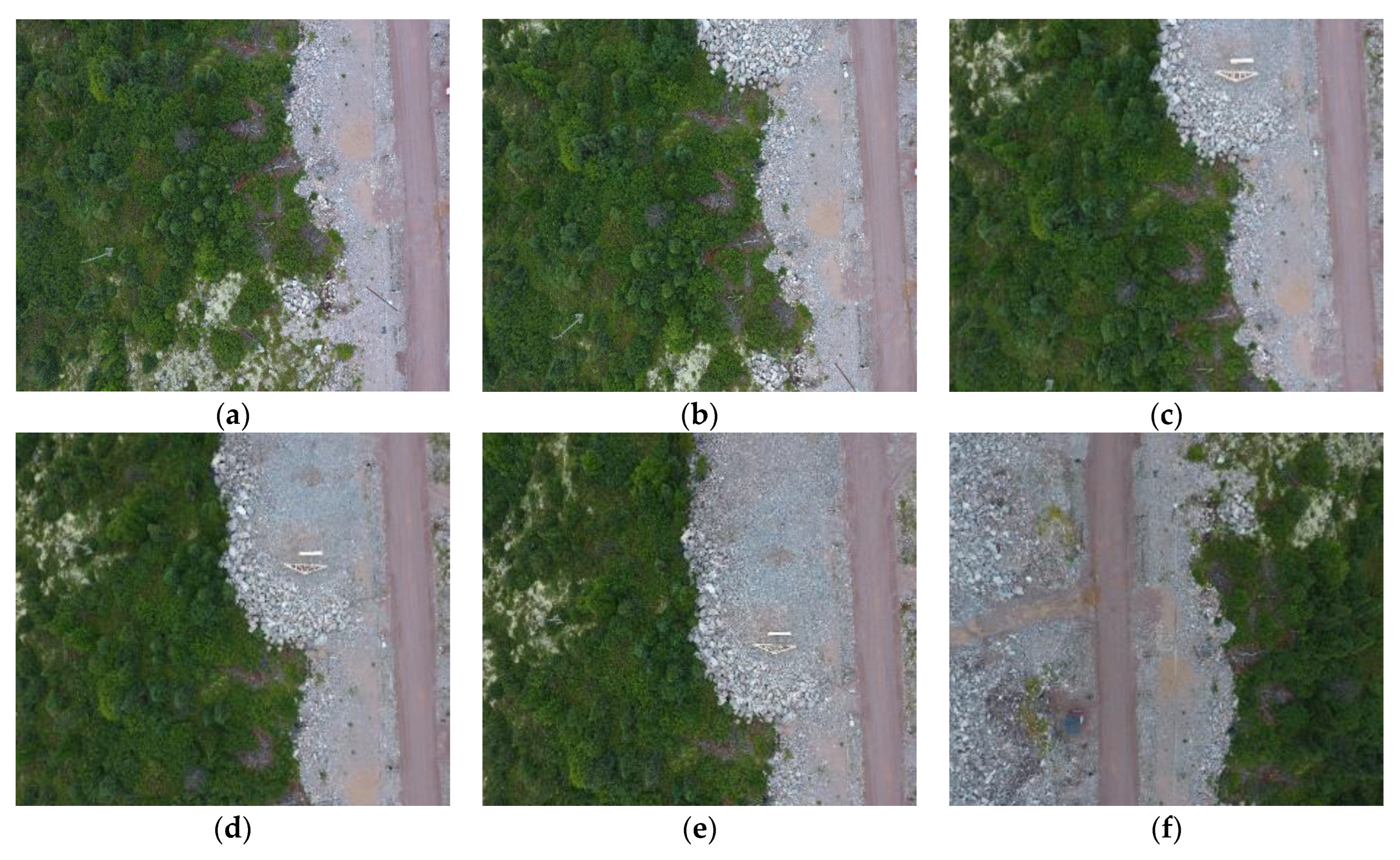
To investigate the potential of the proposed scenarios, first, a freely available dataset [57] was selected. These image pairs have been tested on some of the common state-of-the-art RANSAC-based methods [36,57]. Therefore, we compared our proposed scenarios’ output on this dataset in terms of the accuracy, computational time, and the number of inliers generated by our method with MSAC’s output. The dataset contains image pairs with rotation, scale, and viewpoint changes (Figure 1). For these image pairs, the number of SIFT points is given in Table 1.
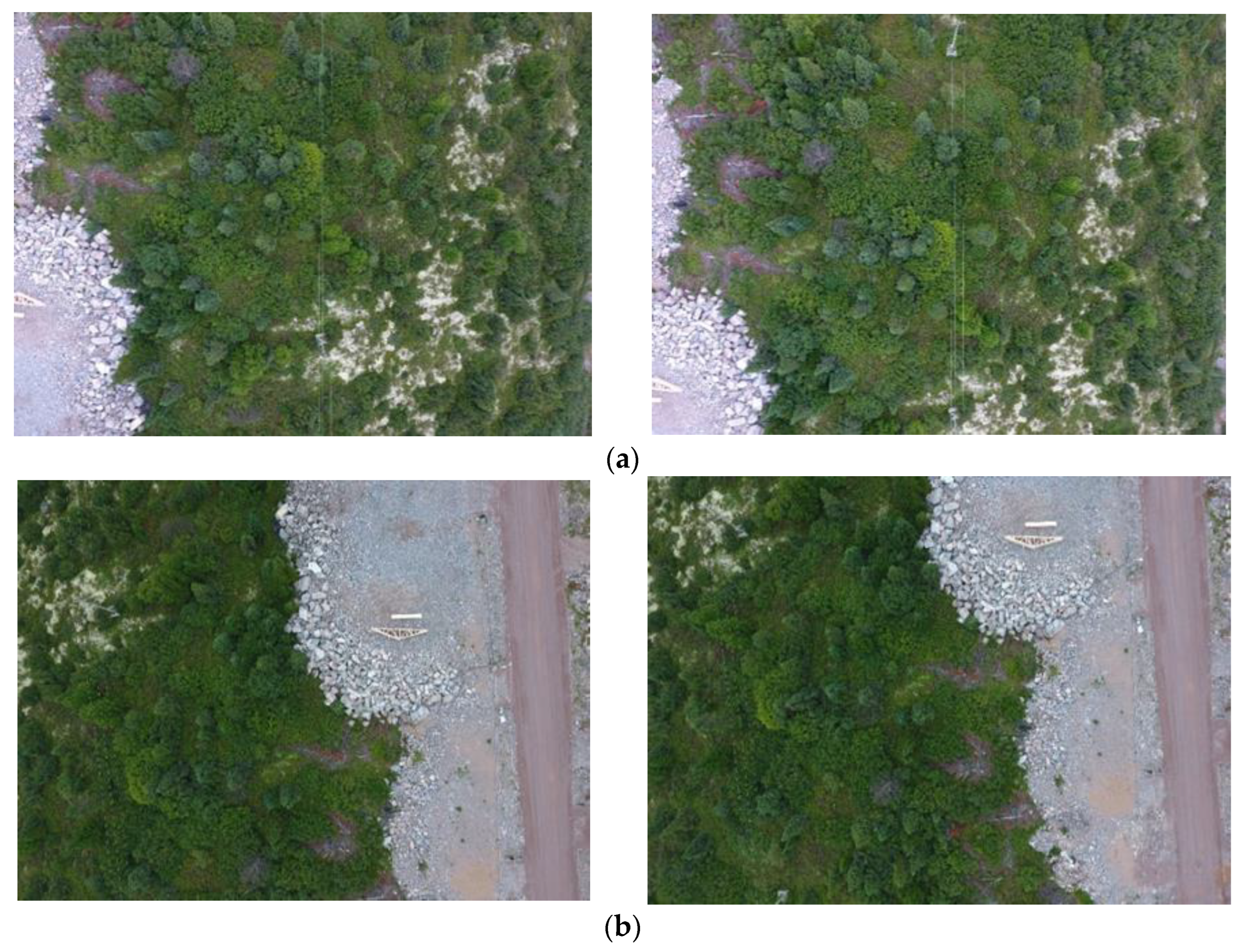
The second dataset consists of image pairs taken by FC330 as a sensor and DJI Phantom 3 as a platform at about a 60-m average flight altitude over an area covered by forest stands (mostly coniferous), clear cuts, roads, and a single building. We purposely picked this area to test the performance of our proposed algorithm in an area containing such land cover types. The parameters of the UAV images are listed in Table 2. Among the acquired UAV images, image pairs with different overlapped, various rotation angle, and different baseline (short to wide) are selected over dense, semi-dense, and sparse forestry areas to assess the proposed enhancements. Figure 2 shows the original images. We compare the accuracy, computational time, and the number of inliers generated by our method with MSAC output. For these image pairs, the number of SIFT points are given in Table 3.

3.2. Performance Evaluation

A total of two scenarios based on different enhancements, Basic and Aggregated LILS, were tested on both datasets. The first scenario combined Basic LILS, AT-Basic, ST-criterion, and PPP. The second scenario combined Aggregated LILS, AT-Improved, ST-criterion, and PPP.
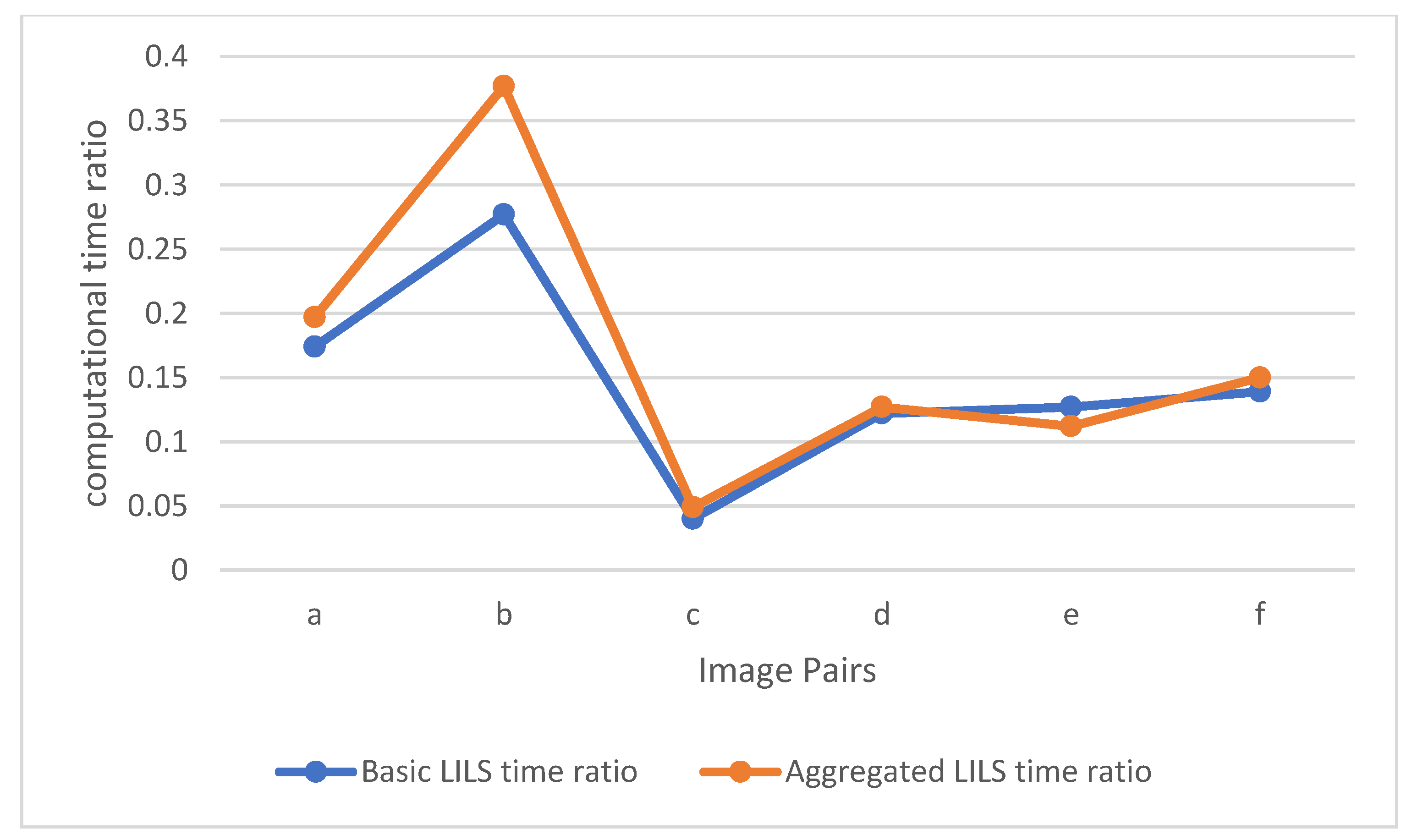
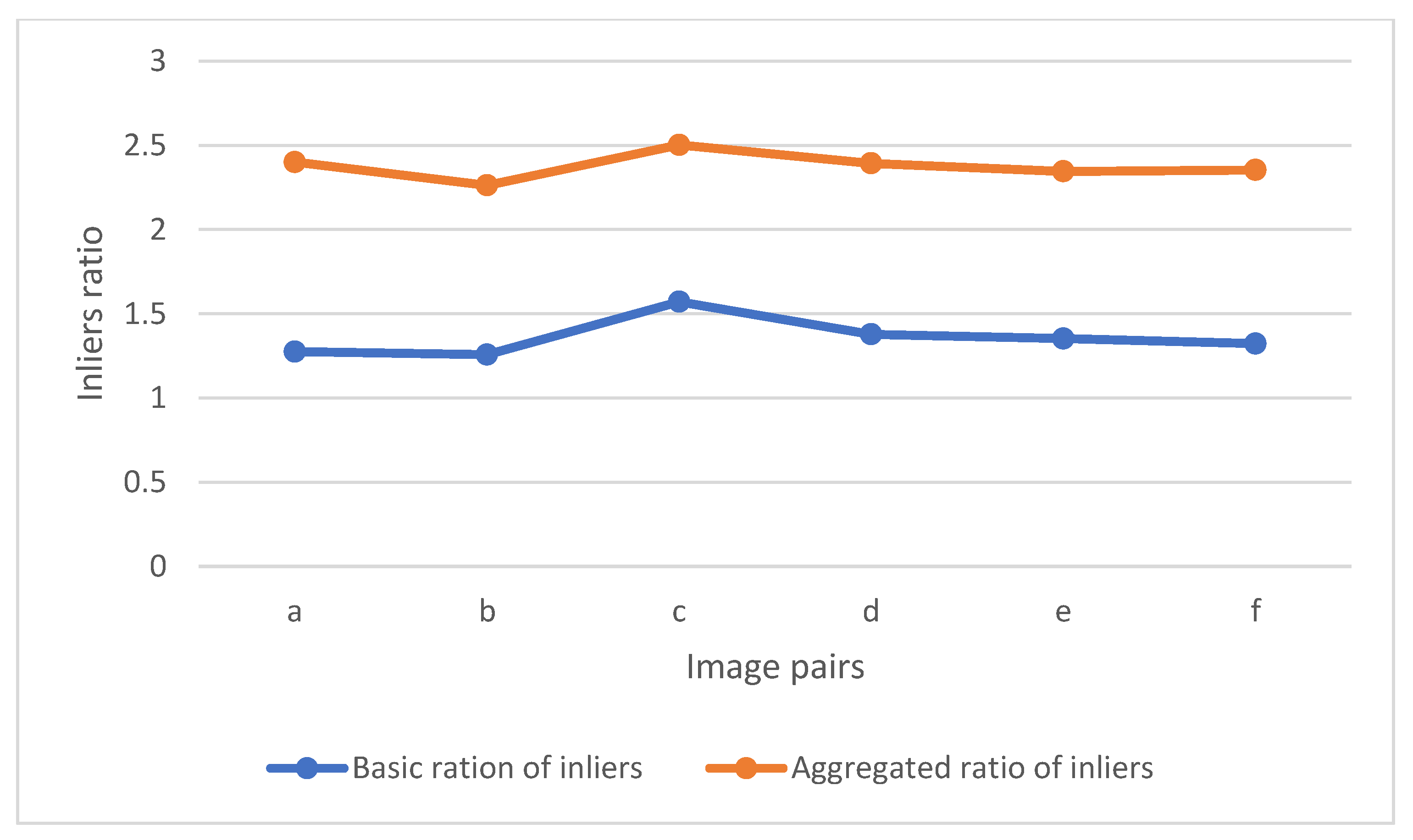
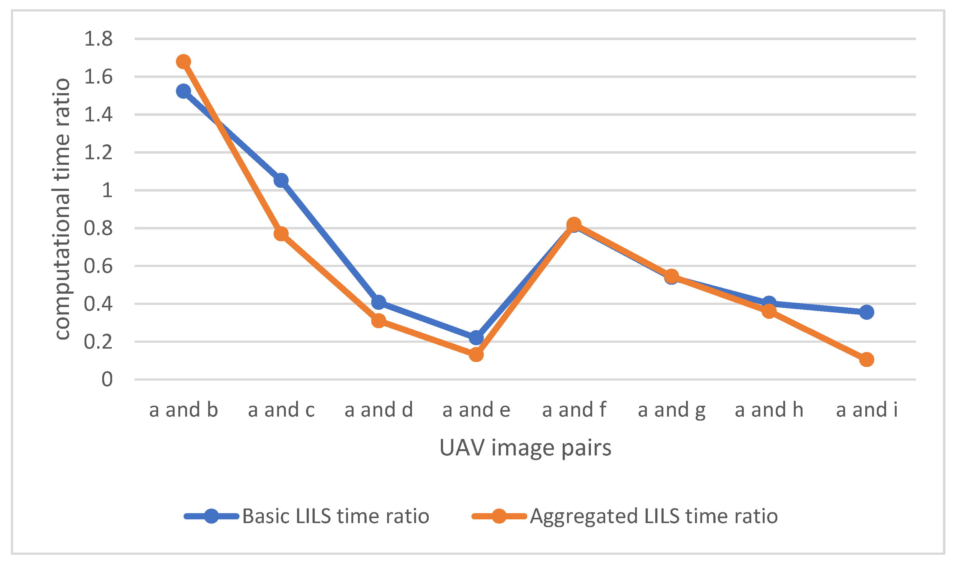
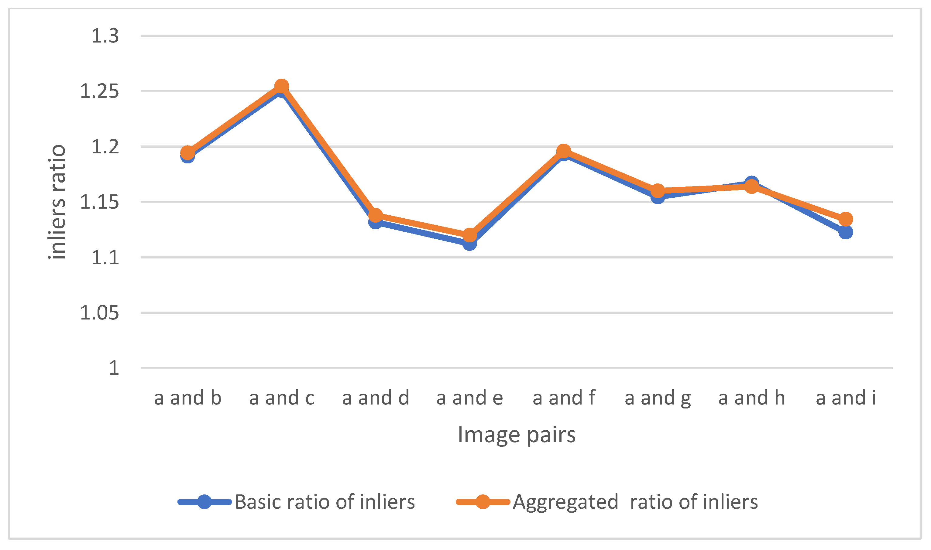
For the performance evaluation of the proposed method, we compared the number of inliers and the computational time for each algorithm with the corresponding values for the MSAC algorithm. To compare the number of inliers, we used the following metrics: the average number of inliers, the minimum number of inliers, maximum number of inliers, and the RMSE of the number of inliers for each image pair. The RMSE was calculated by taking the average RMSE from 100 runs. The relative time ratio to MSAC was reported for the same image pairs. Similar to RMSE, we use the average from 100 runs for the computational time. Table 4 and Table 5 summarize the results for each image pairs in both datasets. Figure 3 and Figure 4 visualize the values reported in Table 4, and Figure 5 and Figure 6 visualize the values reported in Table 5.
As the results suggest, both algorithms (Aggregated and Basic-LILS) find more inliers for all the image pairs than the MSAC, at least 10% more inliers. According to [37,58], the number of required samples (related to the inlier ratios) and the number of data points for the hypothesis evaluation are the main factors that affect the speed of the convergence in RANSAC-based methods. It means that decreasing the inlier ratios, as well as increasing the number of data points, will increase the computational time. Table 4 and Table 5 demonstrate the Basic and Aggregated-LILS loops improve the convergence rate, as well as the stability and the number of inliers.
Table 4 and Table 5 show that, for the proposed algorithm, the number of data points has the strongest effect on increasing the computational time. It means that, by increasing the total number of data points (e.g., a and e), the computational time will increase. Additionally, for both scenarios and datasets, the computational time for all the image pairs is less than the MSAC, except for the UAV dataset’s first image pair (a and b) of the UAV dataset. The potential reason could be the huge number of inliers with respect to the MSAC, approximately 25% more. Further, it is observed that the computational time of the Aggregated-LILS with AT-Improved criteria is less than the computational time for the Basic-LILS with AT-Basic criteria.
It can be observed that all the proposed scenarios behave approximately in a similar manner in terms of the standard deviation of the inliers. In conclusion, the standard deviation of the inliers for all the proposed scenarios is significantly lower than MSAC, which shows both Basic and Aggregated-LILS find approximately similar results in different implementations, disregarding the number of outliers/inliers and type of baselines.

3.3. Point Cloud and DSM Comparison

In order to compare the point cloud and the DSM, we use Aggregated-LILS, as it performs slightly better than Basic-LILS. We chose three different overlapping image pairs over dense, semi-dense, and sparse forestry areas to assess the proposed method. Figure 7 shows the three selected UAV image pairs. To perform the point cloud and DSM comparison, we used commercial Agisoft. The purpose of this study was relative comparison; therefore, the generated products aligned with each other before each assessment using CloudCompare software (Électricité de France, Paris, France).
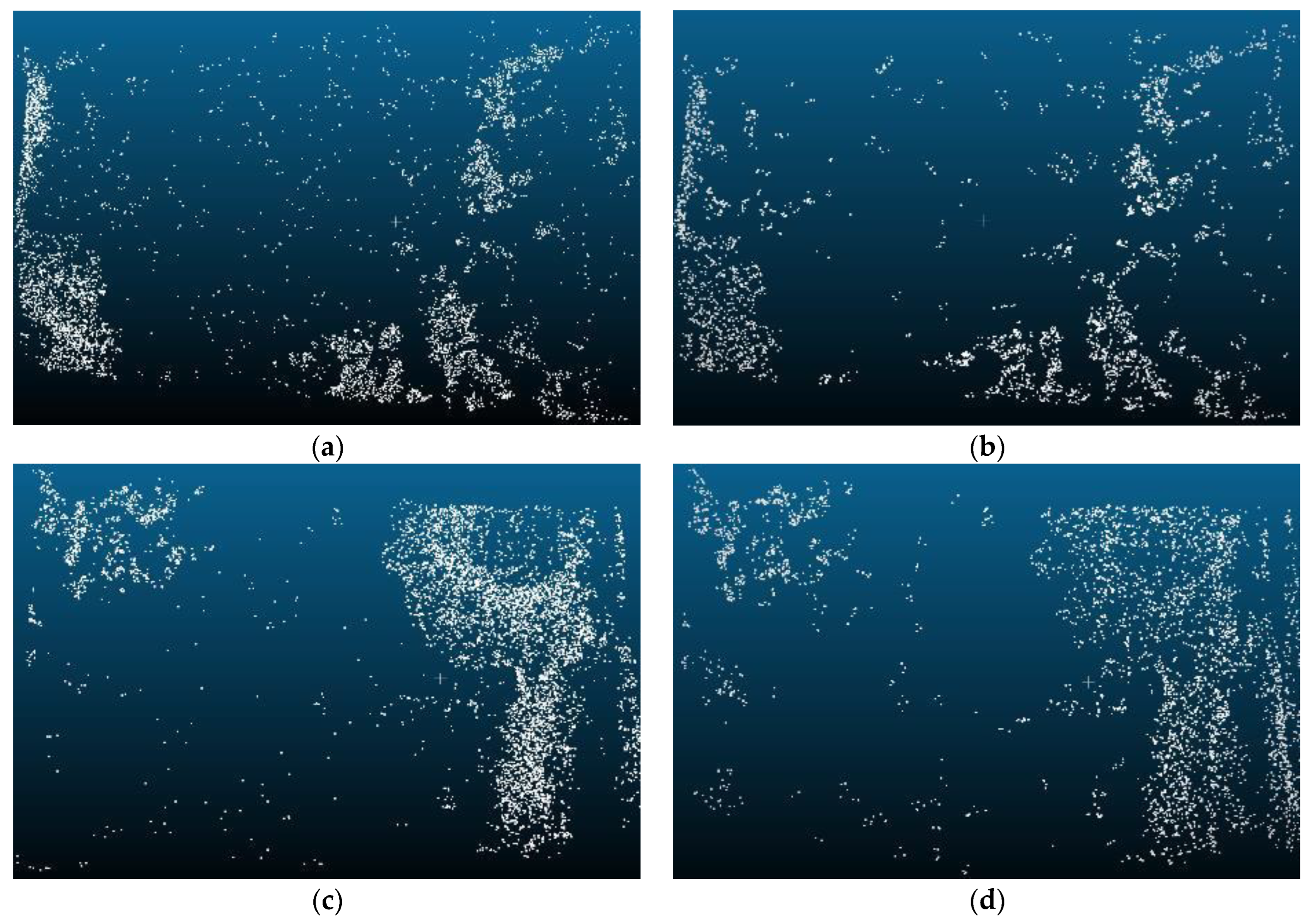
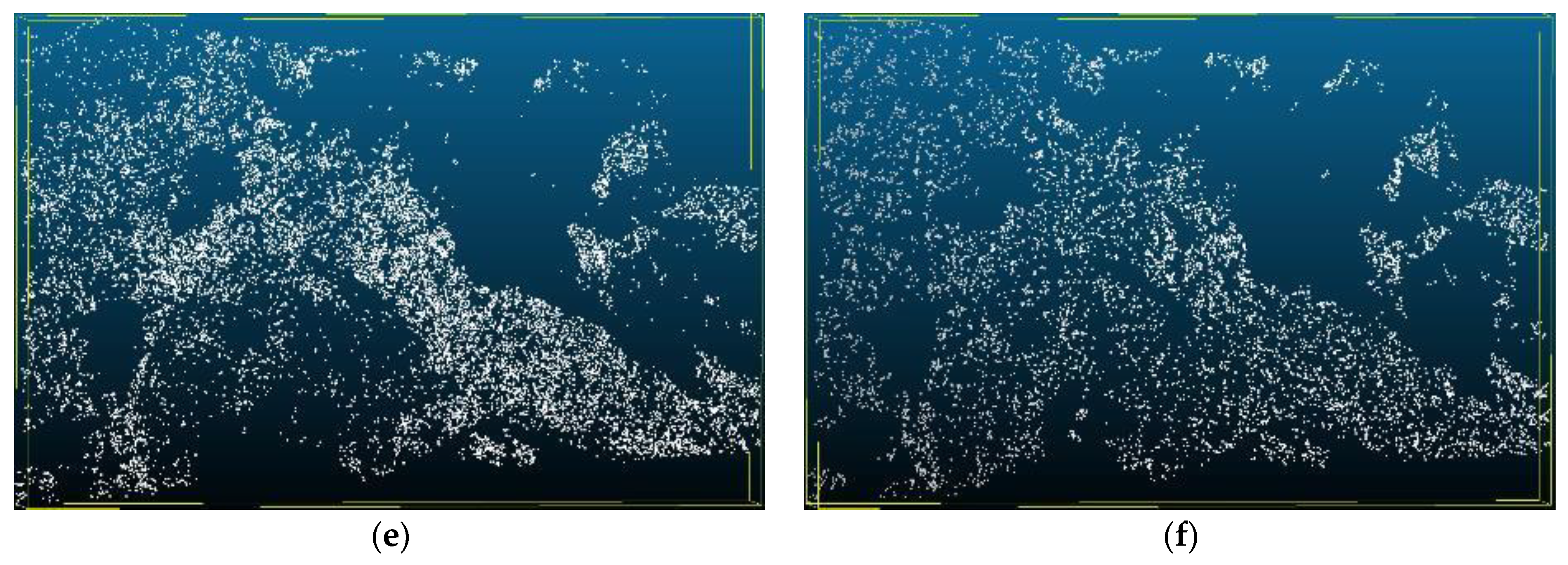
Figure 8 shows the sparse point clouds generated by our proposed method and commercial Agisoft for the selected image pairs. Additionally, Table 6 summarizes the number of inliers in the sparse point clouds generated by each method.
As is shown in Figure 8 and Table 6, the proposed method generates a denser sparse point cloud compared to Agisoft. This was expected, as our method detects more inliers in all the image pairs.
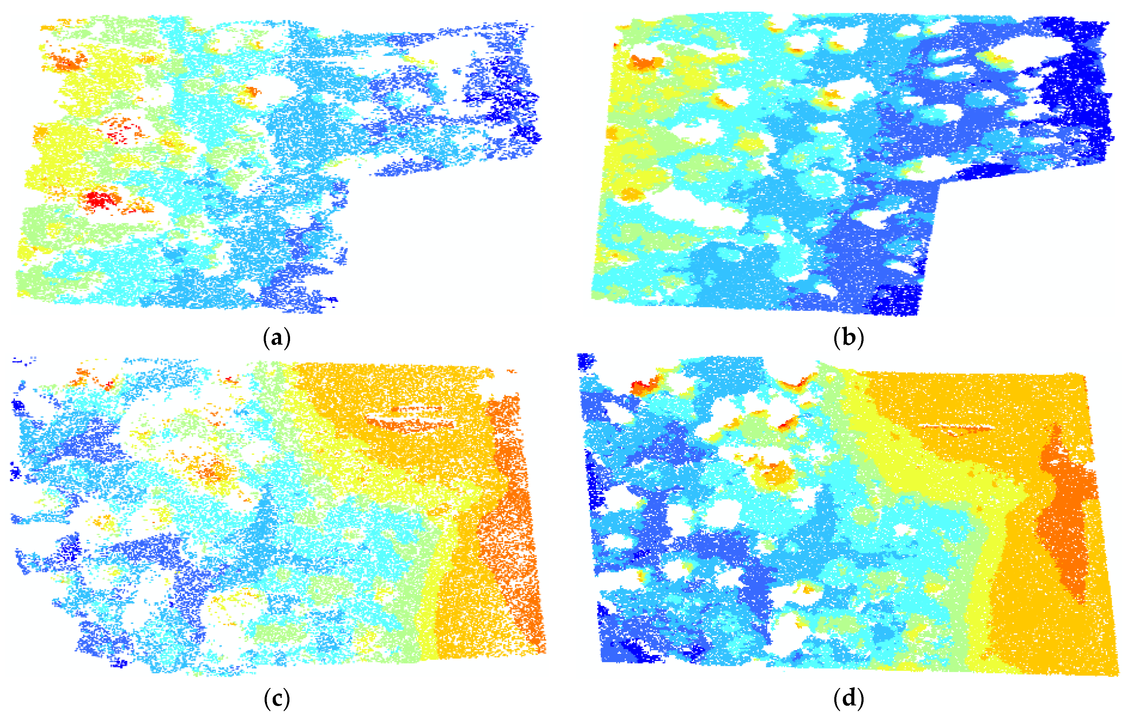
The results after densification are also shown in Figure 9. These point clouds are cropped around the edges to avoid the effect of perspective distortions on the edges of images. The densification of the point clouds based on the proposed procedure is implemented in MATLAB. Due to the memory limitations of MATLAB, our generated dense point clouds have fewer points compared to the dense point clouds of Agisoft.
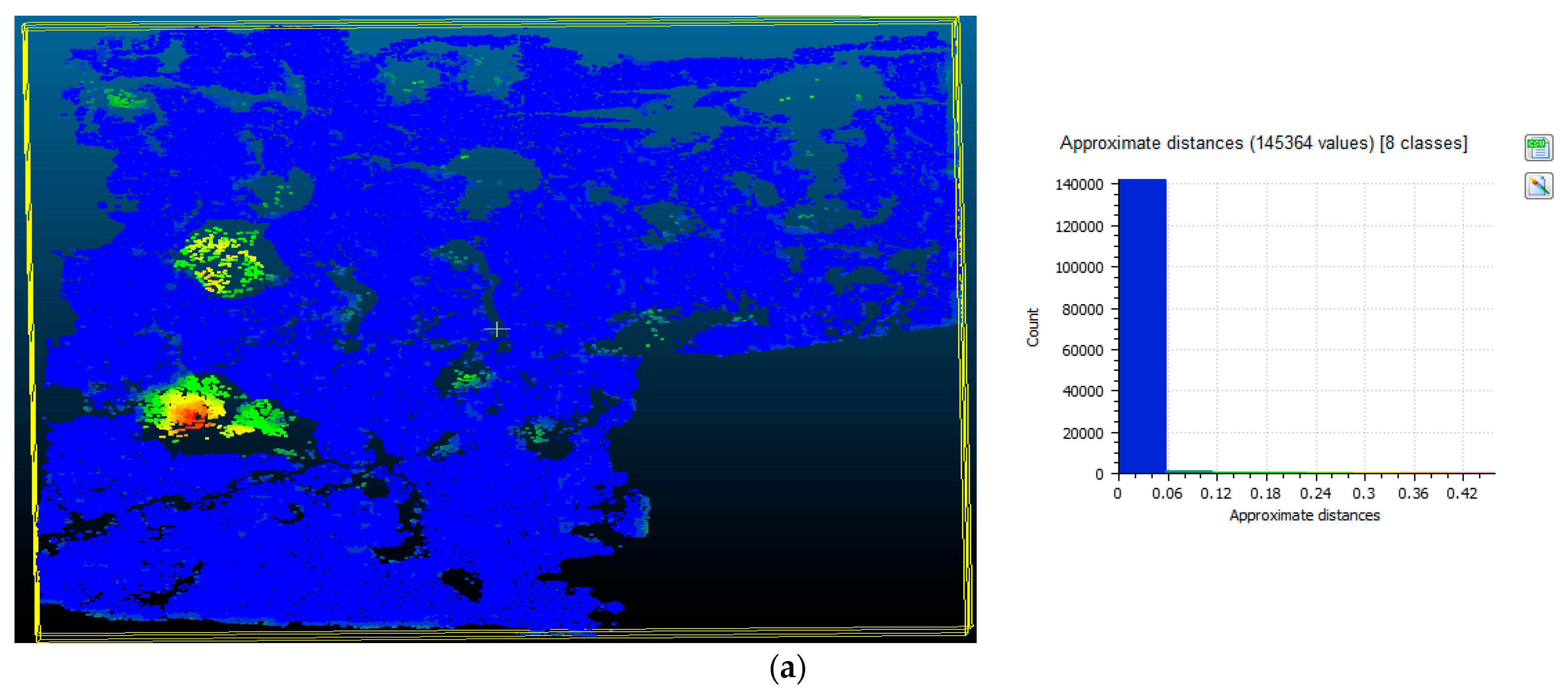
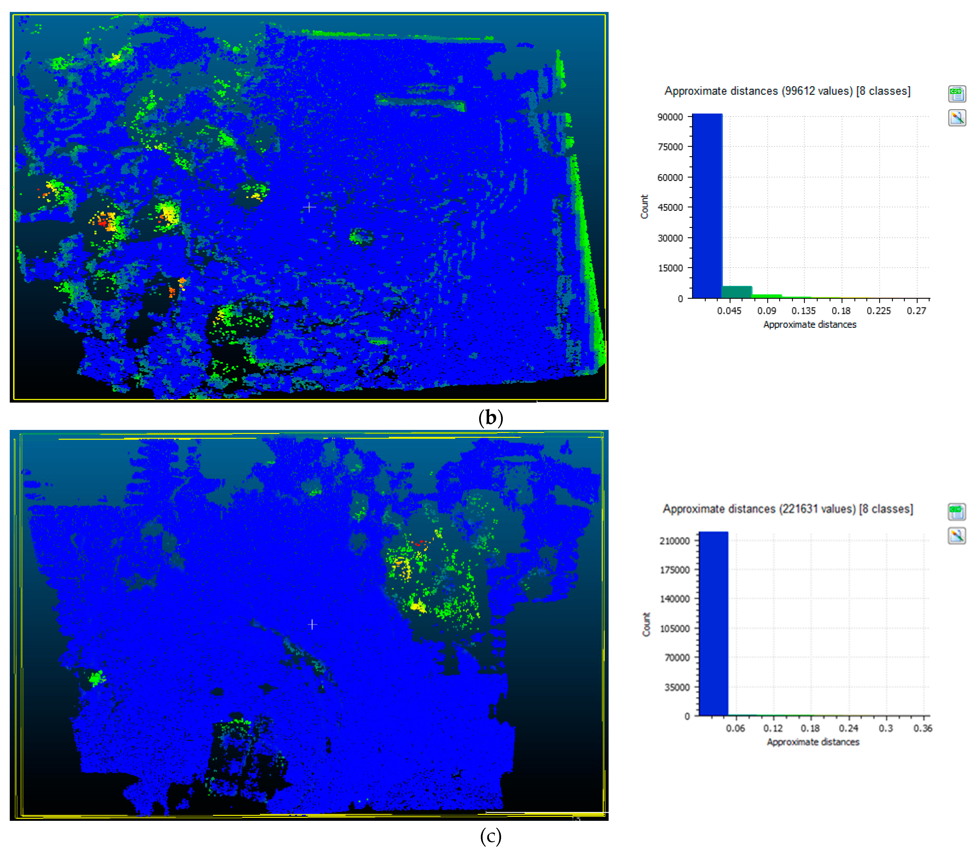
For a better visualization of the difference between the generated dense point clouds, we subtracted the corresponding point clouds using CloudCompare v2.9.alpha (64-bit) software (Électricité de France, Paris, France) based on the Iterative Closest Point (ICP) method. This comparison could also be used to show the elevation differences between two point clouds. Since both dense point clouds are generated using the same images, this difference is used to highlight the areas that are modeled based on the proposed method but not with Agisoft. In Figure 10, similar areas are demonstrated in blue. The visual comparison of both point clouds shows that they match with high percentages in most areas (blue dots in Figure 10). The most significant difference between the two point clouds can be observed in forestry areas, where some single trees were detected in the proposed method but not in the Agisoft point cloud (shown in green, yellow, and red dots in Figure 10).
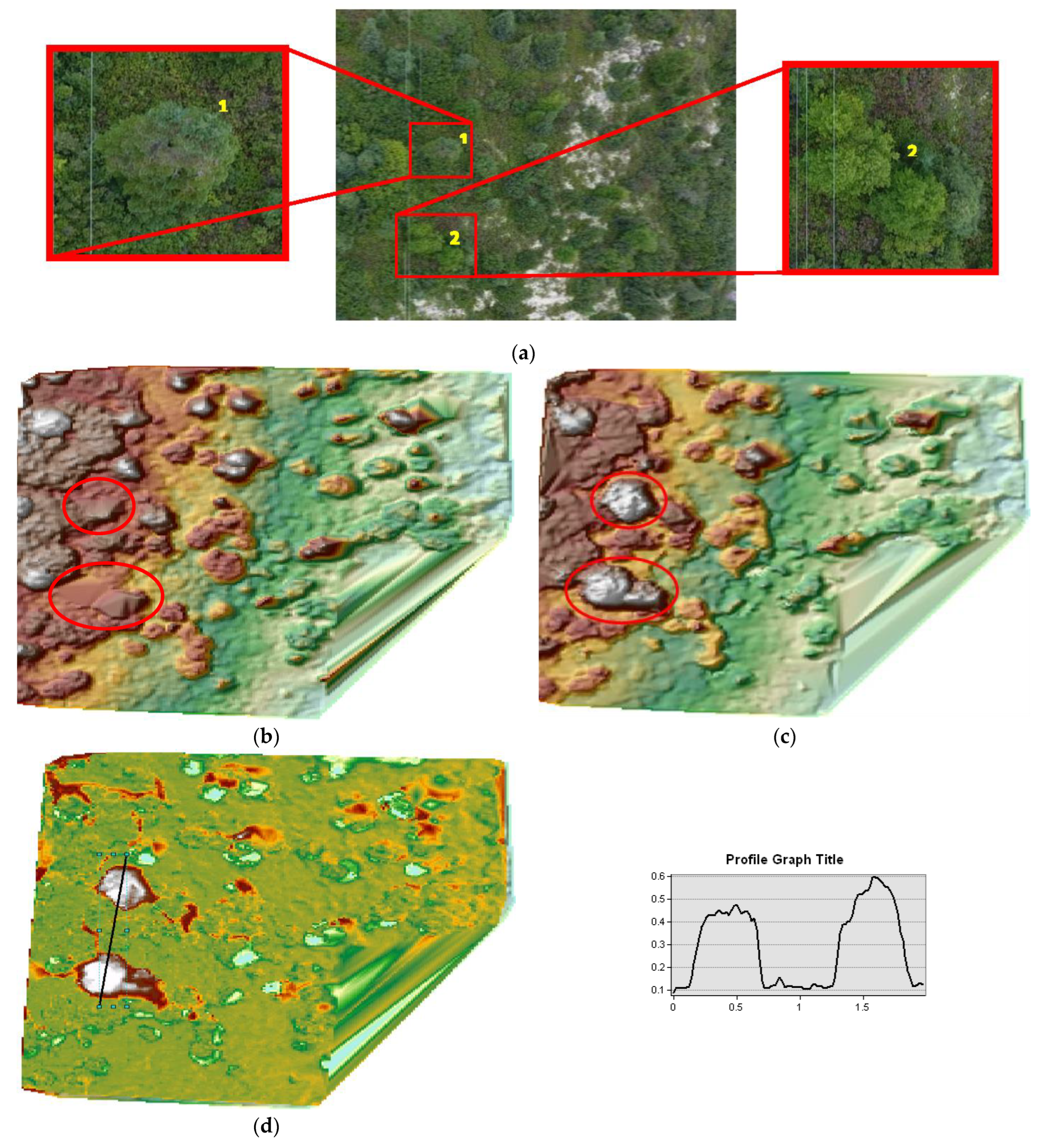
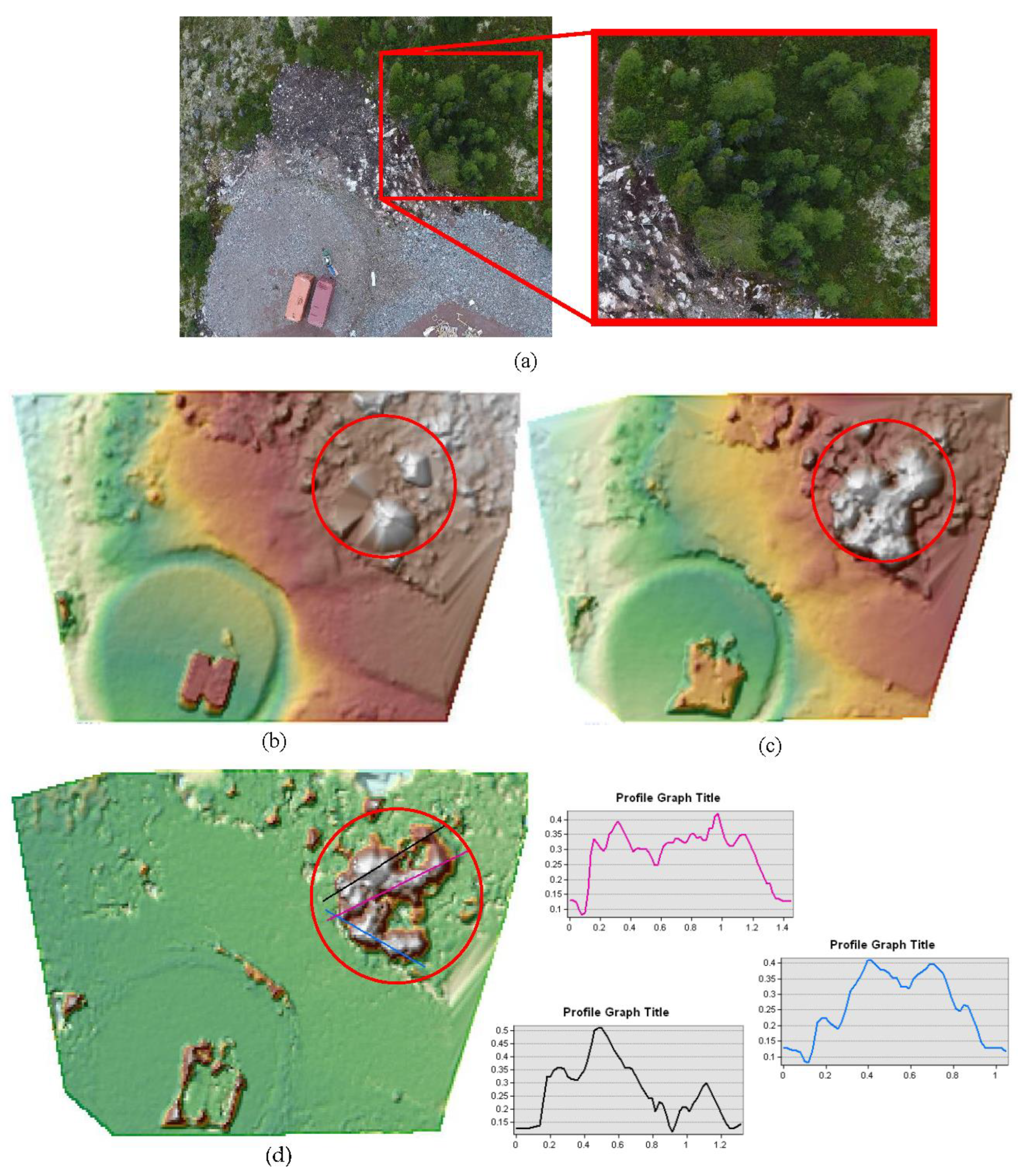
The generated dense point clouds are then used to produce the DSM using ArcGIS 10.5. The results are demonstrated in Figure 11, Figure 12 and Figure 13. In these figures, the trees that are detected by our method, but not with Agisoft, are highlighted with red circles. Additionally, the DSM differences, as well as the profile graphs, are demonstrated. These results show the impact of detecting more inliers in achieving a more detailed point cloud and, consequently, a better DSM in the forestry areas. As can be seen in Figure 11b,c, Figure 12b,c and Figure 13b,c, several trees are detected by our method but not by Agisoft.
The visual comparison of both surfaces (i.e., DSMs) generated from the two methods shows that the proposed procedure is able to detect a more detailed DSM. This comparison shows that some trees are absent from the DSM that is generated by Agisoft. However, the generated DSM based on the proposed method is smoother than that generated using Agisoft. It is because of the lower density of the generated dense point cloud based on the proposed method. As mentioned earlier, this is due to the memory limitations of MATLAB. Therefore, the generated DSM based on the proposed procedure is smoother than those generated by Agisoft. This issue could be fixed by improving the densification procedure in future studies. Generally, it can be said that the proposed procedure performs better in forestry areas by detecting more single trees in comparison to Agisoft.

4. Conclusions

In this paper, we presented a new variant of the RANSAC-based method that improves the performance of RANSAC in terms of increasing the stability, accuracy, the number of inliers, and the convergence rate. Our proposed method, called ELISAC, is based on the combination of three main modifications in the MSAC algorithm; a local iterative least squares-based (LILS) loop to increase the stability and the number of inliers, a similarity termination (ST) criterion to decrease the computational time, and a final post-processing procedure (PPP) to increase the reliability of the results. For this purpose, two scenarios based on different variants of the LILS algorithm (Basic and Aggregated) were tested. The comparative evaluation was done on two computer vision and UAV image pairs with different rotations, scales, and baselines. The results demonstrated that the proposed methods could find more inliers with a faster computational time with respect to the MSAC algorithm. We showed that the proposed method can find and extract more well-distributed inliers and, consequently, generate better point clouds and DSM on UAV image pairs. Moreover, our methods were able to detect and extract more single trees than Agisoft, which could be a direct result of finding more inliers. The proposed modifications are important steps in improving inlier detection and, consequently, generating improved 3D photogrammetric products of UAV data with applications in many areas, including forest 3D mapping. As we tested the ELISAC on a forest area and computer vision dataset, for future works, the ELISAC can test and evaluate other areas, such as urban areas.

Author Contributions

Conceptualization, B.S.; Data curation, B.S.; Formal analysis, S.J.; Project administration, B.S.; Software, S.J.; Supervision, B.S.; Writing—original draft, B.S.; Writing—review & editing, S.J. and A.S. All authors have read and agreed to the published version of the manuscript.

Funding

This project was funded through USDA National Institute of Food and Agriculture (NIFA), McIntire -Stennis grant awarded to the first author.

Institutional Review Board Statement

Not applicable.

Informed Consent Statement

Not applicable.

Data Availability Statement

Not applicable.

Conflicts of Interest

The authors declare that they have no known competing financial interests or personal relationships that could have appeared to influence the work reported in this paper.

References

  1. Gruen, A. Development and Status of Image Matching in Photogrammetry. Photogramm. Rec. 2012, 27, 36–57. [Google Scholar] [CrossRef]
  2. Cramer, M. On the Use of Direct Georeferencing in Airborne Photogrammetry; Citeseer: Princeton, NJ, USA, 2001. [Google Scholar]
  3. Mostafa, M.M.; Hutton, J. Direct Positioning and Orientation Systems: How Do They Work? What Is the Attainable Accuracy. In Proceedings of the Proceedings, The American Society of Photogrammetry and Remote Sensing Annual Meeting, St. Louis, MO, USA, 24–27 April 2001; Citeseer: Princeton, NJ, USA, 2001; pp. 23–27. [Google Scholar]
  4. Mostafa, M.M.; Schwarz, K.-P. Digital Image Georeferencing from a Multiple Camera System by GPS/INS. ISPRS J. Photogramm. Remote Sens. 2001, 56, 1–12. [Google Scholar] [CrossRef]
  5. Poli, D. Indirect Georeferencing of Airborne Multi-Line Array Sensors: A Simulated Case Study. Int. Arch. Photogramm. Remote Sens. Spat. Inf. Sci. 2002, 34, 246–251. [Google Scholar]
  6. Ip, A.W.L. Analysis of Integrated Sensor Orientation for Aerial Mapping; Geomatics Department, University of Calgary: Calgary, AB, Canada, 2005. [Google Scholar]
  7. Ip, A.; El-Sheimy, N.; Mostafa, M. Performance Analysis of Integrated Sensor Orientation. Photogramm. Eng. Remote Sens. 2007, 73, 89–97. [Google Scholar] [CrossRef] [Green Version]
  8. Reshetyuk, Y. Self-Calibration and Direct Georeferencing in Terrestrial Laser Scanning. Ph.D. Thesis, KTH, Stockholm, Sweden, 2009. [Google Scholar]
  9. Kadhim, I.; Abed, F.M. The Potential of LiDAR and UAV-Photogrammetric Data Analysis to Interpret Archaeological Sites: A Case Study of Chun Castle in South-West England. ISPRS Int. J. Geo Inf. 2021, 10, 41. [Google Scholar] [CrossRef]
  10. Li, X.; Xiong, B.; Yuan, Z.; He, K.; Liu, X.; Liu, Z.; Shen, Z. Evaluating the Potentiality of Using Control-Free Images from a Mini Unmanned Aerial Vehicle (UAV) and Structure-from-Motion (SfM) Photogrammetry to Measure Paleoseismic Offsets. Int. J. Remote Sens. 2021, 42, 2417–2439. [Google Scholar] [CrossRef]
  11. Zhang, Y.; Xiong, J.; Hao, L. Photogrammetric Processing of Low-Altitude Images Acquired by Unpiloted Aerial Vehicles. Photogramm. Rec. 2011, 26, 190–211. [Google Scholar] [CrossRef]
  12. Serati, G.; Sedaghat, A.; Mohammadi, N.; Li, J. Digital Surface Model Generation from High-Resolution Satellite Stereo Imagery Based on Structural Similarity. Geocarto Int. 2022, 1–30. [Google Scholar] [CrossRef]
  13. Mohammed, H.M.; El-Sheimy, N. A Descriptor-Less Well-Distributed Feature Matching Method Using Geometrical Constraints and Template Matching. Remote Sens. 2018, 10, 747. [Google Scholar] [CrossRef] [Green Version]
  14. Yao, G.; Yilmaz, A.; Meng, F.; Zhang, L. Review of Wide-Baseline Stereo Image Matching Based on Deep Learning. Remote Sens. 2021, 13, 3247. [Google Scholar] [CrossRef]
  15. Choi, S.; Kim, T.; Yu, W. Performance Evaluation of RANSAC Family. J. Comput. Vis. 1997, 24, 271–300. [Google Scholar]
  16. Fischler, M.A.; Bolles, R.C. Random Sample Consensus: A Paradigm for Model Fitting with Applications to Image Analysis and Automated Cartography. Commun. ACM 1981, 24, 381–395. [Google Scholar] [CrossRef]
  17. Cosgriff, C.V.; Celi, L.A. Deep Learning for Risk Assessment: All about Automatic Feature Extraction. Br. J. Anaesth. 2020, 124, 131–133. [Google Scholar] [CrossRef] [PubMed]
  18. Maggipinto, M.; Beghi, A.; McLoone, S.; Susto, G.A. DeepVM: A Deep Learning-Based Approach with Automatic Feature Extraction for 2D Input Data Virtual Metrology. J. Process Control 2019, 84, 24–34. [Google Scholar] [CrossRef]
  19. Sun, Y.; Yen, G.G.; Yi, Z. Evolving Unsupervised Deep Neural Networks for Learning Meaningful Representations. IEEE Trans. Evol. Comput. 2019, 23, 89–103. [Google Scholar] [CrossRef]
  20. Jin, Y.; Mishkin, D.; Mishchuk, A.; Matas, J.; Fua, P.; Yi, K.M.; Trulls, E. Image Matching across Wide Baselines: From Paper to Practice. Int. J. Comput. Vis. 2021, 129, 517–547. [Google Scholar] [CrossRef]
  21. Ranftl, R.; Koltun, V. Deep Fundamental Matrix Estimation. In Proceedings of the European Conference on Computer Vision (ECCV), Munich, Germany, 17–24 May 2018; pp. 284–299. [Google Scholar]
  22. Sun, W.; Jiang, W.; Trulls, E.; Tagliasacchi, A.; Yi, K.M. Acne: Attentive Context Normalization for Robust Permutation-Equivariant Learning. In Proceedings of the IEEE/CVF Conference on Computer Vision and Pattern Recognition, Seattle, WA, USA, 13–19 June 2020; pp. 11286–11295. [Google Scholar]
  23. Zhang, J.; Sun, D.; Luo, Z.; Yao, A.; Zhou, L.; Shen, T.; Chen, Y.; Quan, L.; Liao, H. Learning Two-View Correspondences and Geometry Using Order-Aware Network. In Proceedings of the IEEE/CVF International Conference on Computer Vision, Seoul, Korea, 27 October–2 November 2019; pp. 5845–5854. [Google Scholar]
  24. Zhao, C.; Cao, Z.; Li, C.; Li, X.; Yang, J. Nm-Net: Mining Reliable Neighbors for Robust Feature Correspondences. In Proceedings of the IEEE/CVF Conference on Computer Vision and Pattern Recognition, Long Beach, CA, USA, 15–20 June 2019; pp. 215–224. [Google Scholar]
  25. Liu, J.; Wang, S.; Hou, X.; Song, W. A Deep Residual Learning Serial Segmentation Network for Extracting Buildings from Remote Sensing Imagery. Int. J. Remote Sens. 2020, 41, 5573–5587. [Google Scholar] [CrossRef]
  26. Zhu, Y.; Zhou Sr, Z.; Liao Sr, G.; Yuan, K. New Loss Functions for Medical Image Registration Based on Voxelmorph. In Proceedings of the Medical Imaging 2020: Image Processing, SPIE, Houston, TX, USA, 15–20 February 2020; Volume 11313, pp. 596–603. [Google Scholar]
  27. Cao, Y.; Wang, Y.; Peng, J.; Zhang, L.; Xu, L.; Yan, K.; Li, L. DML-GANR: Deep Metric Learning with Generative Adversarial Network Regularization for High Spatial Resolution Remote Sensing Image Retrieval. IEEE Trans. Geosci. Remote Sens. 2020, 58, 8888–8904. [Google Scholar] [CrossRef]
  28. Yang, Y.; Li, C. Quantitative Analysis of the Generalization Ability of Deep Feedforward Neural Networks. J. Intell. Fuzzy Syst. 2021, 40, 4867–4876. [Google Scholar] [CrossRef]
  29. Wang, L.; Qian, Y.; Kong, X. Line and Point Matching Based on the Maximum Number of Consecutive Matching Edge Segment Pairs for Large Viewpoint Changing Images. Signal Image Video Process. 2022, 16, 11–18. [Google Scholar] [CrossRef]
  30. Zheng, B.; Qi, S.; Luo, G.; Liu, F.; Huang, X.; Guo, S. Characterization of Discontinuity Surface Morphology Based on 3D Fractal Dimension by Integrating Laser Scanning with ArcGIS. Bull. Eng. Geol. Environ. 2021, 80, 2261–2281. [Google Scholar] [CrossRef]
  31. Zhang, X.; Zhu, X. Efficient and De-Shadowing Approach for Multiple Vehicle Tracking in Aerial Video via Image Segmentation and Local Region Matching. J. Appl. Remote Sens. 2020, 14, 014503. [Google Scholar] [CrossRef]
  32. Xiuxiao, Y.; Wei, Y.; Shu, X.U.; Yanhua, J.I. Research Developments and Prospects on Dense Image Matching in Photogrammetry. Acta Geod. Cartogr. Sin. 2019, 48, 1542. [Google Scholar]
  33. Bellavia, F.; Colombo, C.; Morelli, L.; Remondino, F. Challenges in Image Matching for Cultural Heritage: An Overview and Perspective. In Proceedings of the FAPER 2022, Springer LNCS, Lecce, Italy, 23–24 May 2022. [Google Scholar]
  34. Salehi, B.; Jarahizadeh, S. Improving the uav-derived dsm by introducing a modified ransac algorithm. Int. Arch. Photogramm. Remote Sens. Spat. Inf. Sci. 2022, 43, 147–152. [Google Scholar] [CrossRef]
  35. Torr, P.H.; Zisserman, A. MLESAC: A New Robust Estimator with Application to Estimating Image Geometry. Comput. Vis. Image Underst. 2000, 78, 138–156. [Google Scholar] [CrossRef] [Green Version]
  36. Chum, O.; Matas, J.; Kittler, J. Locally Optimized RANSAC. In Proceedings of the Joint Pattern Recognition Symposium, Madison, WI, USA, 16–22 June 2003; Springer: Berlin/Heidelberg, Germany, 2003; pp. 236–243. [Google Scholar]
  37. Chum, O.; Matas, J. Matching with PROSAC-Progressive Sample Consensus. In Proceedings of the 2005 IEEE Computer Society Conference on Computer Vision and Pattern Recognition (CVPR’05), San Diego, CA, USA, 20–25 June 2005; IEEE: Piscataway, NJ, USA, 2005; Volume 1, pp. 220–226. [Google Scholar]
  38. Frahm, J.-M.; Pollefeys, M. RANSAC for (Quasi-) Degenerate Data (QDEGSAC). In Proceedings of the 2006 IEEE Computer Society Conference on Computer Vision and Pattern Recognition (CVPR’06), New York, NY, USA, 17–22 June 2006; IEEE: Piscataway, NJ, USA, 2006; Volume 1, pp. 453–460. [Google Scholar]
  39. Hast, A.; Nysjö, J.; Marchetti, A. Optimal Ransac-towards a Repeatable Algorithm for Finding the Optimal Set. J. WSCG 2013, 21, 21–30. [Google Scholar]
  40. Raguram, R.; Chum, O.; Pollefeys, M.; Matas, J.; Frahm, J.-M. USAC: A Universal Framework for Random Sample Consensus. IEEE Trans. Pattern Anal. Mach. Intell. 2012, 35, 2022–2038. [Google Scholar] [CrossRef]
  41. Barath, D.; Matas, J.; Noskova, J. MAGSAC: Marginalizing Sample Consensus. In Proceedings of the IEEE/CVF Conference on Computer Vision and Pattern Recognition, Long Beach, CA, USA, 15–20 June 2019; pp. 10197–10205. [Google Scholar]
  42. Korman, S.; Litman, R. Latent Ransac. In Proceedings of the IEEE Conference on Computer Vision and Pattern Recognition, Salt Lake City, UT, USA, 18–23 June 2018; pp. 6693–6702. [Google Scholar]
  43. Chum, O.; Werner, T.; Matas, J. Two-View Geometry Estimation Unaffected by a Dominant Plane. In Proceedings of the 2005 IEEE Computer Society Conference on Computer Vision and Pattern Recognition (CVPR’05), San Diego, CA, USA, 20–25 June 2005; IEEE: Piscataway, NJ, USA, 2005; Volume 1, pp. 772–779. [Google Scholar]
  44. Barath, D.; Matas, J. Graph-Cut RANSAC. In Proceedings of the IEEE Conference on Computer Vision and Pattern Recognition, Salt Lake City, UT, USA, 18–23 June 2018; pp. 6733–6741. [Google Scholar]
  45. Zhang, D.; Zhu, J.; Wang, F.; Hu, X.; Ye, X. GMS-RANSAC: A Fast Algorithm for Removing Mismatches Based on ORB-SLAM2. Symmetry 2022, 14, 849. [Google Scholar] [CrossRef]
  46. Le, V.-H.; Vu, H.; Nguyen, T.T.; Le, T.-L.; Tran, T.-H. Acquiring Qualified Samples for RANSAC Using Geometrical Constraints. Pattern Recognit. Lett. 2018, 102, 58–66. [Google Scholar] [CrossRef]
  47. Raguram, R.; Frahm, J.-M.; Pollefeys, M. A Comparative Analysis of RANSAC Techniques Leading to Adaptive Real-Time Random Sample Consensus. In Proceedings of the European Conference on Computer Vision, Marseille, France, 12–18 October 2008; Springer: Berlin/Heidelberg, Germany, 2008; pp. 500–513. [Google Scholar]
  48. AgiSoft PhotoScan Pro; Agisoft LLC: Saint Petersburg, Russia, 2021.
  49. Han, J.-Y.; Guo, J.; Chou, J.-Y. A Direct Determination of the Orientation Parameters in the Collinearity Equations. IEEE Geosci. Remote Sens. Lett. 2011, 8, 313–316. [Google Scholar] [CrossRef]
  50. Szeliski, R. Structure from Motion and SLAM. In Computer Vision; Springer: Berlin/Heidelberg, Germany, 2022; pp. 543–594. [Google Scholar]
  51. Elnima, E.E. A Solution for Exterior and Relative Orientation in Photogrammetry, a Genetic Evolution Approach. J. King Saud Univ. Eng. Sci. 2015, 27, 108–113. [Google Scholar] [CrossRef] [Green Version]
  52. Adjidjonu, D.; Burgett, J. Assessing the Accuracy of Unmanned Aerial Vehicles Photogrammetric Survey. Int. J. Constr. Educ. Res. 2021, 17, 85–96. [Google Scholar] [CrossRef]
  53. Rais, M.; Facciolo, G.; Meinhardt-Llopis, E.; Morel, J.-M.; Buades, A.; Coll, B. Accurate Motion Estimation through Random Sample Aggregated Consensus. arXiv 2017, arXiv:1701.05268. [Google Scholar]
  54. Lindeberg, T. Scale Invariant Feature Transform. Comput. Sci. 2012, 7, 10491. [Google Scholar] [CrossRef]
  55. Hartley, R.I. In Defense of the Eight-Point Algorithm. IEEE Trans. Pattern Anal. Mach. Intell. 1997, 19, 580–593. [Google Scholar] [CrossRef] [Green Version]
  56. Zhang, H.; Ye, C. Sampson Distance: A New Approach to Improving Visual-Inertial Odometry’s Accuracy. In Proceedings of the 2021 IEEE/RSJ International Conference on Intelligent Robots and Systems (IROS), Prague, Czech Republic, 27 September–1 October 2021; pp. 9184–9189. [Google Scholar]
  57. Lebeda, K.; Matas, J.; Chum, O. Fixing the Locally Optimized Ransac–Full Experimental Evaluation. In Proceedings of the British Machine Vision Conference, Surrey, UK, 3–7 September 2012; Citeseer: Princeton, NJ, USA, 2012; Volume 2. [Google Scholar]
  58. Chum, O.; Matas, J. Optimal Randomized RANSAC. IEEE Trans. Pattern Anal. Mach. Intell. 2008, 30, 1472–1482. [Google Scholar] [CrossRef] [PubMed] [Green Version]
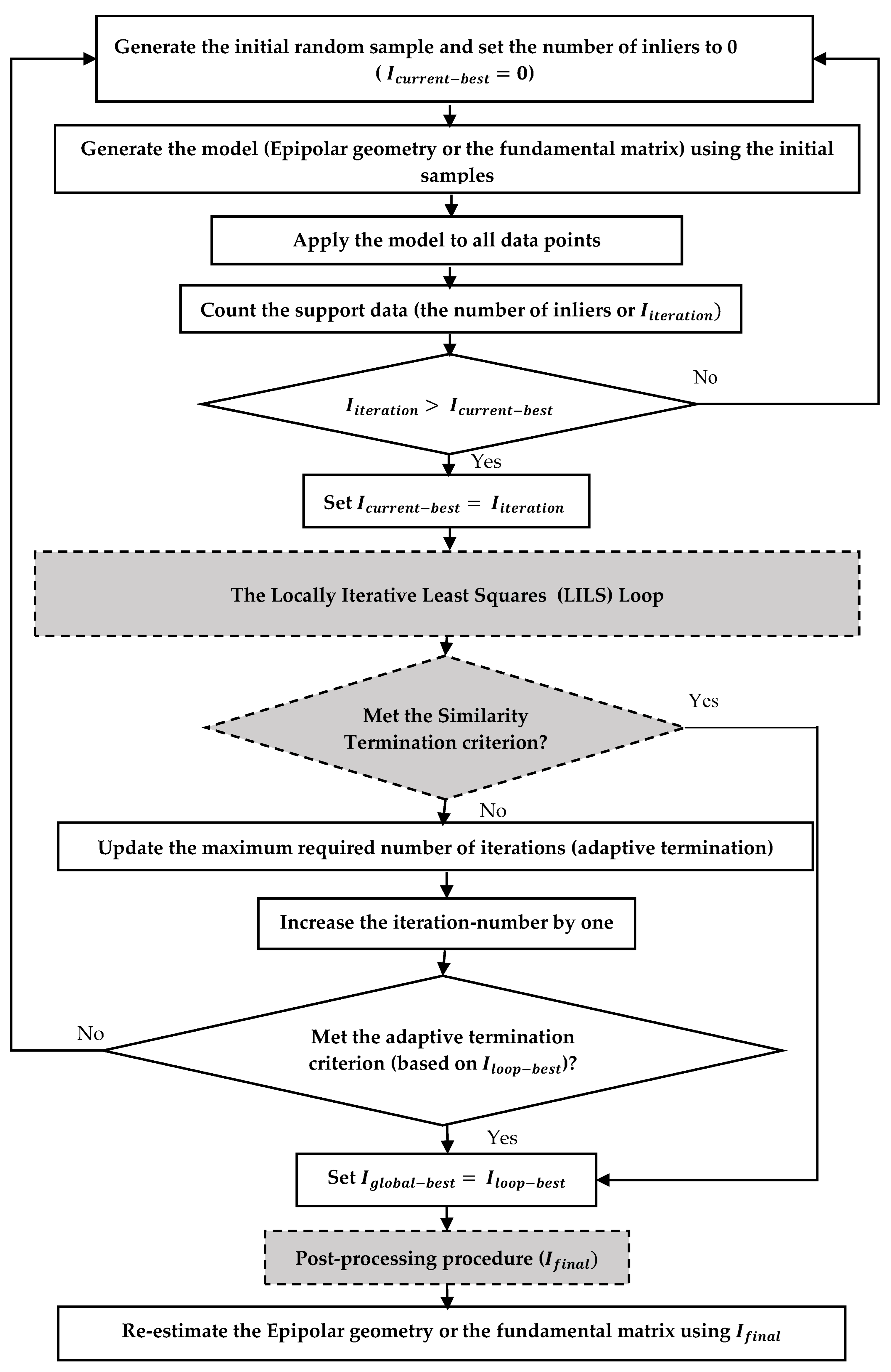
Chart 1. Processing steps in MSAC and the proposed ELISAC method (gray boxes show the three enhancements steps).
Remotesensing 14 04917 ch001
Figure 1. The image samples of the first dataset (Books (a), Box (b), Kampa (c), Kyoto (d), Plant (e), Valbonne (f)).
Remotesensing 14 04917 g001
Figure 2. The image sequence samples of the UAV dataset (image pairs: (a,b), (a,c), (a,d), (a,e), (a,f), (a,g), (a,h), and (a,i)).
Remotesensing 14 04917 g002aRemotesensing 14 04917 g002b
Figure 3. Ratio of the computational time with respect to MSAC for the first dataset.
Remotesensing 14 04917 g003
Figure 4. Ratio of inliers with respect to MSAC for the first dataset.
Remotesensing 14 04917 g004
Figure 5. Ratio of computational time with respect to MSAC for the UAV dataset.
Remotesensing 14 04917 g005
Figure 6. Ratio of inliers with respect to MSAC for the UAV dataset.
Remotesensing 14 04917 g006
Figure 7. Three different stereo UAV images over dense (a), semi-dense (b), and sparse (c) forestry areas.
Remotesensing 14 04917 g007aRemotesensing 14 04917 g007b
Figure 8. The generated sparse point cloud by the proposed procedure (a–c) and Agisoft (d–f) from the first, second, and third datasets, respectively.
Remotesensing 14 04917 g008aRemotesensing 14 04917 g008b
Figure 9. The generated dense point clouds based on the proposed procedure (a–c) and Agisoft (d–f) from the first, second, and third datasets.
Remotesensing 14 04917 g009aRemotesensing 14 04917 g009b
Figure 10. The differences between the generated point clouds by Agisoft and the proposed method from (a) the first, (b) second, and (c) third datasets.
Remotesensing 14 04917 g010aRemotesensing 14 04917 g010b
Figure 11. The image captured at the desired area (a), the generated DSM by Agisoft (b), as well as the proposed method, (c) are also shown from the first dataset. The subtraction of two DSMs, in addition to the profile graph, is also demonstrated (d).
Remotesensing 14 04917 g011
Figure 12. The image captured at the desired area (a), the generated DSM by Agisoft (b), as well as the proposed method, (c) are also shown from the second dataset. The subtraction of two DSMs, in addition to the profile graph, is also demonstrated (d).
Remotesensing 14 04917 g012
Figure 13. The image captured at the desired area (a), the generated DSM by Agisoft (b), as well as the proposed method, (c) are also shown from the third dataset. The subtraction of two DSMs, in addition to the profile graph, is also demonstrated (d).
Remotesensing 14 04917 g013
Table 1. The number of match points of the first dataset image pairs.
Image PairsBooks (a)Box (b)Kampa (c)Kyoto (d)Plant (e)Valbonne (f)
Number of SIFT points16741822773015797
Table 2. The UAV image pair specifications.
Weight (g)1280
Diagonal size (mm)350
Max speed (m/s)16
UAV modelDJI Phantom 3
CameraModelFC330
Sensor1/2.3″ CMOS (Effective pixels: 12.4 M)
LensFOV 94°20 mm
Hover Accuracy RangeVertical±0.5 m (with GPS Positioning)
Horizontal±1.5 m (with GPS Positioning)
Max. flight time (minute)23
Image size (pixels)4000 × 3000
Ground resolution size of images (cm/pix)2
Average flight altitude (m)53.8
Focal length in 35 mm format (mm)20
ISO speed174
Exposure1/60
Aperture Value2.8
Image area coverage (m2)81 × 61
Table 3. The number of match points of UAV image pairs.
Image Pairsa and ba and ca and da and ea and fa and ga and ha and i
Number of SIFT points779126211083420426524001324728
Table 4. The obtained results from all image pairs in the first dataset.
Books (a)Box (b)Kampa (c)Kyoto (d)Plant (e)Valbonne (f)
Inliers’ average-RMSE
I(min-max)
MSAC80.0 ± 5.6
(67–93)
221.7 ± 9.8
(200–247)
70.1 ± 3.6
(61–79)
245.7 ± 10.1
(214–266)
52.1 ± 4.1
(41–63)
39.1 ± 2.3
(30–44)
Basic LILS102.0 ± 6.0
(84–118)
278.7 ± 15.2
(234–303)
110.1 ± 8.8
(85–136)
338.5 ± 28.6
(257–392)
70.45 ± 5.4
(56–83)
51.7 ± 4.1
(39–61)
Aggregated LILS90.0 ± 6.9
(71–98)
222.8 ± 15.6
(186–249)
65.3 ± 4.9
(53–79)
249.4 ± 12.7
(202–266)
51.7 ± 4.8
(41–64)
40.3 ± 3.5
(31–46)
Ratio of inliers w.r.t MSACBasic LILS1.2751.25711.57061.37761.35221.3222
Aggregated LILS1.1251.00490.93151.0150.99231.0306
Ratio of computational time w.r.t MSACBasic LILS0.1740.2770.0400.1220.1270.139
Aggregated LILS0.1970.3770.0490.1270.1120.150
Table 5. The obtained results from all image pairs (a and b, a and c, a and d, a and e, a and f, a and g, a and h, and a and i).
a and ba and ca and da and ea and fa and ga and ha and i
Inliers’ average-RMSE
(min-max)
MSAC4516.5 ± 245.9
(4001–5128)
1374.3 ± 68.2
(1228–1566)
491.3 ± 20.1
(447–552)
119.2 ± 4.7
(104–131)
2416.1 ± 130.5
(2145–2699)
1243.3 ± 66.4
(1100–1383)
618.8 ± 30.0
(540–688)
248.6 ± 10.5
(227–274)
Basic LILS5380.4 ± 51.4
(4935–5420)
1593.6 ± 35.8
(1511–1644)
556.1 ± 8.0
(531–570)
132.6 ± 2.5
(124–137)
2882.9 ± 14.4
(2828–2909)
1435.5 ± 14.3
(1384–1463)
722.1 ± 11.9
(681–743)
279.1 ± 7.0
(243–290)
Aggregated LILS5394.4 ± 19.8
(5301–5439)
1598.8 ± 34.7
(1456–1644)
559.1 ± 7.5
(538–571)
133.5 ± 2.7
(123–139)
2889.5 ± 13.2
(2844–2913)
1442.3 ± 16.7
(1380–1478)
720.2 ± 13.6
(680–746)
282.0 ± 7.4
(260–296)
Ratio of inliers w.r.t MSACBasic LILS1.19121.25051.13181.11241.19321.15451.16691.1226
Aggregated LILS1.19431.25461.13801.11991.19591.16001.16381.1343
Ratio of computational time w.r.t MSACBasic LILS1.5221.0510.4070.2200.8140.5390.4020.355
Aggregated LILS1.6780.7690.3100.1310.8190.5450.3600.105
Table 6. The number of inliers.
MethodNumber of Points in the Generated Sparse Point Clouds
First Dataset (a)Second Dataset (b)Third Dataset (c)
The proposed procedure4870575511,292
Agisoft software330642257418
Publisher’s Note: MDPI stays neutral with regard to jurisdictional claims in published maps and institutional affiliations.