Abstract
On the basis of 12 years of the European Centre for Mesoscale Weather Forecasts (ECMWF) reanalysis dataset, we statistically analyzed the spatiotemporal distribution of lower atmospheric ducts over the seas around China, and we investigated the possible generation mechanisms. The results show that the ducts’ occurrence had obvious seasonal and regional variations. Ducting events were more likely to occur in spring and summer, and the maximum occurrence rate reached 45.6%, which was closely related to the East Asian monsoon. The ducts’ altitude in continental coastal areas was lower than that far from the coast due to the dominance of surface ducts. The ducts’ thickness varied between 50 m and 450 m, and the thicker ducts were mainly concentrated in the South China Sea and the Pacific Ocean on the east side of the East China Sea near the Philippines and Taiwan. Except for a few areas, the ducts’ intensity was less than 10 M-units (an M-unit is the unit of atmospheric modified refractivity) and the diurnal variations were less pronounced. The duct formation in the lower atmosphere was related to factors such as monsoons, tropical cyclones, ocean currents, radiative cooling, and sea–land breezes.
1. Introduction
When the atmospheric layer meets certain conditions, radio waves are trapped and propagated in an approximately horizontal duct, which is called an atmospheric duct. Atmospheric ducts are generally divided into three types: evaporation ducts, surface ducts, and elevated ducts [1,2]. Different physical mechanisms are associated with the formation of different duct types [2,3]. Evaporation ducts are induced by strong humidity and temperature gradients caused by intensive evaporation at the air–sea interface, and their altitude is generally less than 40 m [2,4]. Surface ducts are typically generated by advection when warm dryland air passes over a cooler sea [3]. The warm air over cold water forms a surface-based inversion, with moisture decreasing rapidly with height, resulting in a substantial negative M gradient in the lowest levels. Nocturnal radiation cooling over land can also produce strong temperature inversions and surface ducts [3]. Elevated ducts can be caused by temperature inversions aloft, generated by the sinking or subsidence of air masses [5]. Moreover, elevated ducts can be also induced by strong daytime surface heating when strong turbulence eddies are capped by a higher inversion [6]. Surface ducts and elevated ducts are called lower atmospheric ducts.
Atmospheric ducts frequently occur at the marine boundary layer, and they significantly affect radar systems, communication systems, and navigation systems by changing the propagation path and attenuation characteristics of electromagnetic waves through, for example, propagation loss, transmission fading, reductions/increases in the detection range, and shortening/expansion of radio horizons [7,8]. The influence of atmospheric ducts on radio waves is closely related to the ducts’ parameters [9]. Studying the spatiotemporal distribution of atmospheric ducts is helpful for the design and development of radio communication systems to provide environmental analysis information and auxiliary decision-making tools.
In recent years, ducting events have been extensively studied around the world by using different datasets. Patterson [10] reported on duct climatology around the world based on 6-year radiosonde data. Babin [3] statistically analyzed the seasonal variations in surface ducts over the Atlantic Ocean near Wallops Island, Virginia, using low-altitude refractive data measured by helicopters. The results showed that during spring and autumn, the surface ducts’ occurrence rate was higher and the average duct altitude was the largest. Brooks [11] presented the spatial variations in the boundary layer structure and duct intensity over the Persian Gulf by using the observation data of ships and aircraft in 1996. Mentes et al. [12] made a statistical analysis of seasonal and local variations in surface ducts over Istanbul, Turkey, by using 2-year radiosonde data. They believed that the ducts’ occurrence strongly depended on the prevailing weather and meteorological conditions in the local region. Ghouse Basha [13] used 5 years of high-resolution GPS radiosonde observation data to analyze the parameters of ducts over Gadanki, indicating that the ducts’ occurrence had obvious diurnal and seasonal variations, and the ducts’ altitude in a stable state was higher than that in the unstable state. Zhao [14] and Cheng [15] conducted similar research on lower atmospheric ducts over the South China Sea and the eastern Indian Ocean by using sounding observation data taken during cruises.
Although sounding/radiosonde data are commonly used in statistical analyses of atmospheric ducts, they have the limitations of lower coverage and resolution in time and space. ECMWF reanalysis data can make up for the deficiencies in of sounding/radiosonde data. Von Engeln et al. [16] studied the seasonal and temporal variations in the global occurrence, altitude, thickness, and intensity of ducts based on the 6-year ERA-40 reanalysis data of ECMWF, and showed the global duct climatology. Lopez [17] carried out a global duct climatological study based on 5 years of assimilation data from the ECMWF, and they summarized the mainly climatic features of global ducts. Sirkova et al. [18] reported the occurrence and properties of ducts along the Black Sea coast of Bulgaria based on ECMWF model data. Cheng et al. [19] also used ERA-I data to statistically analyze the monthly variations in and climatological features of lower atmospheric ducts over the South China Sea. Their research showed that the distribution of atmospheric ducts was not uniform, with obvious regional and seasonal variations.
In view of the important influence of atmospheric ducts on wireless electronic information systems and the difficulty of obtaining the sounding data of marine atmospheric ducts, we used the ERA-5 hourly data to study the spatiotemporal distribution of lower atmospheric ducts’ parameters over the seas adjacent to China. The main objectives were as follows. Firstly, the parameters of lower atmospheric ducts were counted to establish a lower atmospheric duct environment database in the region and to provide a reference for the design and deployment of radar and communication systems in this region. Secondly, we aimed to study the synoptic conditions and formation mechanisms of the atmospheric ducts to provide a scientific basis for analyzing, forecasting, and utilizing the atmospheric ducts. Finally, the study provided parameter inputs and a reference for establishing a microwave propagation prediction model of this area in our future work.
2. Data and Statistical Methods
2.1. Data Description
ERA5 data are the latest climate and atmosphere reanalyses produced by the ECMWF. They provide atmospheric parameters with a temporal resolution of 1 h and a horizontal resolution of 0.25° × 0.25° at 37 pressure levels from 1000 hPa (about 70 m) to 1 hPa (about 48 km) [20]. More detailed information about the ERA5 data can be found in the ERA5 Data Documentation Report (https://cds.climate.Copernicus.eu/, accessed on 26 September 2021). In this study, we selected the ERA5 data on the region covering the geographical latitude and longitude swath of 0–42°N and 105–132°E from January 2008 to September 2020 to study the spatiotemporal distribution of lower atmospheric ducts over the seas adjacent to China (a map of the seas adjacent to China is provided in the Supplementary Material). Since most duct events occur below 2 km and the maximum duct altitude is about 5 km [21,22], we selected temperature, specific humidity, pressure, and geopotential parameters at 14 pressure levels from 1000 hPa to 600 hPa (about 4.5 km) for this study.
2.2. Statistical Methods
The occurrence of atmospheric ducts is caused by changes in atmospheric refractivity. The relationship of atmospheric refractivity and temperature, pressure, and water vapor pressure is shown in the following formula [23,24]:
where N is the atmospheric refractivity (N-units), P is the atmospheric pressure (hPa), T is the temperature (K), and e is the water vapor pressure (hPa). Among these, the water vapor pressure e can be calculated from the specific atmospheric humidity [18]:
where q is the specific humidity (g/kg) and is a constant (0.622).
The modified refractivity M, corrected by the curvature of the Earth, is given by the formula of Bean and Dutton [23]:
where M is the atmospheric modified refractivity (M-units), Re is the average radius of the Earth (6371 km), and h is the altitude above sea level (m).
The atmospheric refraction types are classified as sub-refraction, standard refraction, super-refraction, and trapping (ducting) according to the gradient of refractivity N or the gradient of modified refractivity M [2,17]. A trapping layer or duct occurs when the modified refractivity gradient M is negative [25,26]. The relationship between the N gradient and the M gradient is shown in Table 1.

Table 1.
The relationship between N gradient and M gradient in different Refraction types.
Because the evaporation ducts’ altitude is usually less than 40 m, the vertical resolution of the ERA5 data is insufficient to capture evaporation ducting events. Therefore, we only investigated the spatiotemporal distribution of the parameters of lower atmospheric ducts over the seas around China. In lower atmospheric ducts, there are not only single surface ducts or elevated ducts, but also combinations of multiple ducts, namely composite ducts [2,27]. In previous duct event research, only the first duct near the ground was considered [5,16,19], while the case of composite ducts was not considered. It is worth mentioning that here, we also conducted a statistical analysis of composite ducts.
Figure 1 shows the types and parameters of classical lower atmospheric ducts [1], including a surface duct (Figure 1a), a surface-based duct (Figure 1b), an elevated duct (Figure 1c), and a composite duct (Figure 1d).
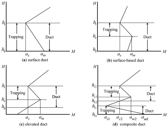
Figure 1.
Schematic diagram of lower atmospheric duct types and parameters: (a) surface duct; (b) surface-based duct; (c) elevated duct; (d) composite duct.
The steps of calculating the duct parameters of each atmospheric refractivity profile were as follows:
- Calculate the double-weighted average and standard deviation of all the temperature, pressure, and specific humidity profiles, then eliminate the profiles with greater than four standard deviations from the mean [28].
- Interpolate the temperature, pressure, specific humidity, and geopotential profiles to a 20 m resolution in the vertical by cubic-spline interpolation [29]. It should be noted that the altitude can be obtained by the geopotential of each pressure level. The altitude can be calculated by the following formula:where G is the geopotential (m2/s2) and g is the gravitational acceleration (m2/s2). Here, g is a constant (9.80665 m/s2). The modified refractivity M profiles were calculated by Formulas (1)–(3). An interpolation result is shown in Figure 2.
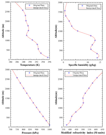 Figure 2. Comparison of the temperature, pressure, specific humidity, and modified refractivity profiles before and after interpolation. Data for the comparison were selected at 14.25°N, 110.50°E on 9 January 2008 at UTC 19:00.
 - Use the central difference method to calculate the vertical gradient of the modified refractivity M at each height:where i is the vertical point index of each profile. The total number of M profiles we calculated was (4657 × 24 × (42/0.25 + 1) × (27/0.25 + 1). The number 4657 indicates the days.
- Judge if a composite duct appears in each M′(i) profile. The method of judging whether a composite duct has occurred involves counting the number of trapping layers in each M′(i) profile. If there are two or more trapping layers in a M′(i) profile, a composite duct has occurred in the observation period.
- Record the duct parameters in each M′(i) profile individually, then check the value of M′(i) from bottom to top. When M′(i) < 0, the altitude is defined as the bottom of the trapping layer he. When M′(i) begins to change from M′(i) < 0 to M′(i) > 0, the altitude is defined as the top of the trapping layer ht. The trapping layer lies between ht and he. As shown in Figure 1a–c, the duct’s altitude is ht, the duct’s thickness is ht − hm, and the duct’s intensity is am − as.
- Arrange the duct’s parameter data into grids with a latitude–longitude resolution of 1° × 1°, then calculate the average value of the duct parameters within each grid.
- Finally, analyze the seasonal variations and monthly features of, and the diurnal variations in the ducts’ parameters. The seasons are divided into spring (March, April, and May), summer (June, July, and August), autumn (September, October, and November), and winter (December, January, and February). The diurnal variations included four local times: LT00, LT06, LT12, and LT18. The formula for calculating local time is given as follows:where LT is the local time, UTC is the Coordinated Universal Time, and long is the longitude (deg) of M profiles in the range of −180° to 180°.
3. Statistical Results and Discussion
3.1. Duct Occurrence Rate
The occurrence rate of atmospheric ducts is defined as the number of M profiles where ducts occurred divided by the total number of M profiles in each grid. Figure 3 shows the spatiotemporal distribution of the occurrence rate of lower atmospheric ducts over the seas around China.
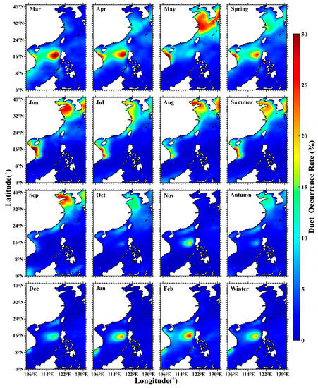
Figure 3.
Distribution of the duct occurrence rate, with monthly and seasonal variations.
The marine areas adjacent to China are extensive, spanning temperate, subtropical, and tropical climate zones. Because of the effect of climate and geography, the occurrence of ducts has obvious seasonal variations and regional distribution characteristics, which can be clearly seen in Figure 3.
In spring, the areas where ducts are prone to occur were mainly concentrated in the northwest of the South China Sea, the eastern coastal areas of China, and the Yellow Sea. The duct occurrence rate in these areas over the East China Sea, the Yellow Sea, and the Bohai Sea increased significantly from May to September, which was consistent with the period when the East Asian summer monsoon prevails (May to September) [30]. April and May are the transition period of the East Asian monsoon from winter circulation to summer circulation. At this time, the North Pacific Subtropical High controls the North Pacific, and the southerly monsoon begins to prevail in the Yellow Sea and the Bohai Sea, with high temperature and humidity [30]. When warm and humid air advection cools water bodies, this causes temperature and humidity inversions, which lead to the formation of ducts in the upper parts of the Marine Atmospheric Boundary Layer (MABL) [3,13]. Unlike the ducts that occurred in the Yellow Sea and the Bohai Sea, the duct coverage areas over the South China Sea decreased sharply in May, which was consistent with Cheng’s [19] results. Between April and July, the duct occurrence rate in the eastern coastal seas of Indo-China Peninsula was always higher, which was related to the downslope subsidence caused by the offshore summer monsoon [19]. Affected by the winter monsoon, the duct occurrence rate in the South China Sea was always lower than 10%.
In summer, the areas with a higher duct occurrence rate were mainly concentrated in continental coastal waters. The duct occurrence rate gradually decreased as the distance from the coastline increased. The main reason for this phenomenon is that the radiation inversions and local circulation (such as sea–land breezes) were caused by intense solar radiation, which advected dry and warm air from the land to cold and wet seas, forming surface ducts in coastal areas [31]. This is why the ducts’ altitude in the continental coastal areas was generally lower than that over open seas in summer. Von Engeln [16] indicated that the development of fog during the warmer seasons may lead to a higher probability of ducting events on the east coast of Asia. Zhang [32] pointed out that sea fog over the Yellow Sea was prevalent from April to August, which is roughly the same as the period of higher duct occurrence rates in the Yellow Sea.
October and November are the periods when the summer monsoon changes to the winter monsoon; the Mongolian High controls and affects the offshore seas of China, making the sea surface isobar lines show a northeast–southwest trend, and the wind direction is stable and northward [30]. During this time, the seas become gradually controlled by the high pressure caused by continental cold. The atmospheric humidity is relatively lower, which is not conducive to duct formation. Through the effects of the winter monsoon, the duct occurrence rate was less than 10% between October and next March in the Bohai Sea, the Yellow Sea, and the East China Sea (Figure 3). At about the same time, the duct occurrence rate northwest of the Philippines was higher than that in summer, which may be related to frequent tropical cyclone activity. According to Chen [30], the areas from Luzon Island in the Philippines to Hainan Island at 15–20°N have the most frequent tropical cyclone activity. Ziemba [6] and Ding [33] both indicated that ducts occur frequently in areas affected by tropical storms and hurricanes.
Figure 4 shows the monthly variations in the proportion of surface ducts, elevated ducts, and composite ducts within total ducting events. Surface ducts dominated in all months, and had a maximum occurrence rate between June and August and a minimum occurrence rate in March. This also explains the phenomenon of lower duct altitudes over the coastal seas of Mainland China in summer. Elevated ducts appeared most frequently in March. Figure 5 shows the monthly variations in the number of composite ducting events, showing that the largest number of composite ducts occurred in July.
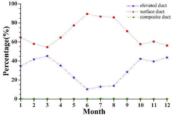
Figure 4.
Monthly variations in the proportion of surface, elevated, and composite ducts within total ducting events.
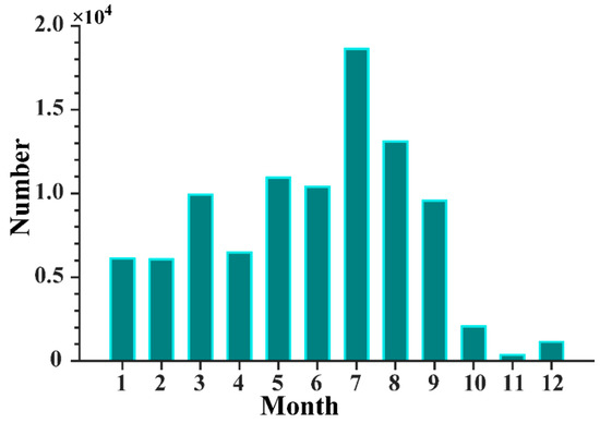
Figure 5.
Monthly variations in the number of composite ducts.
In order to study the daily variations in the ducts’ occurrence, we grouped the ducting events according to the local time (LT00, LT06, LT12, and LT18). The statistical results are shown in Figure 6. In general, the ducts appeared in fixed locations, mainly concentrated in the coastal areas of Mainland China and the northwest of the Philippines. The diurnal variations in the duct occurrence rate were more obvious in the Bohai–Yellow Sea area, the western seas of the Philippines, and the eastern coastal areas of the Indo-China Peninsula. The duct occurrence rate and the ducts’ coverage areas were greater in the evening than during the day. If we take the eastern coastal seas of the Indo-China Peninsula as an example, at LT12, the duct occurrence rate was less than 18%, with a small coverage area. At LT18, the duct occurrence rate increased by 6% and the duct areas covered most of the eastern coastal waters in the Indo-China Peninsula. However, at LT00, sea–land breezes were formed by radiation cooling, and the land breeze brought dry and cold air to the sea surface, forming an inversion layer [13,34], which helped to generate ducts.

Figure 6.
Distribution of the duct occurrence rate across different local times.
3.2. Duct Altitude
The duct altitude usually refers to the altitude of the top of the trapping layer. In Figure 1a–c, ht is the duct altitude. A composite duct’s altitude is ht1 and ht2, as shown in Figure 1d. Duct altitude has an important effect on the propagation of radio waves. Figure 7 shows the seasonal and monthly variations in duct altitude over the seas around China.
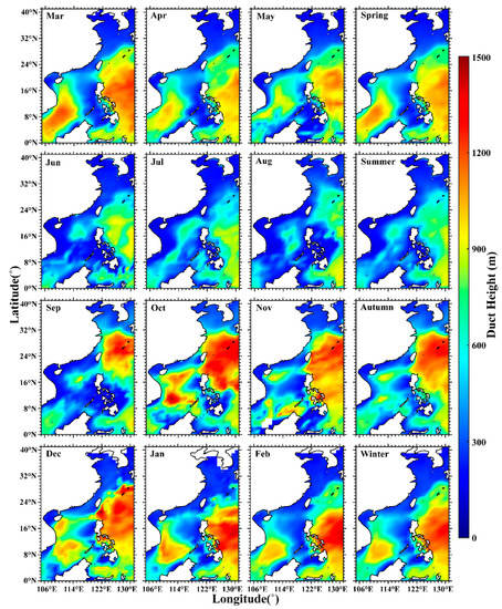
Figure 7.
Distribution of duct altitude, with monthly and seasonal variations.
The seasonal and monthly variations in duct altitude are obvious in Figure 7. The duct altitude was the highest in autumn and winter, while the lowest occurred in summer. The duct altitude was less than 250 m in the Bohai Sea and the north of the Yellow Sea all year round. Except for minor areas in the north of Taiwan and the South China Sea, the duct altitude was lower than 300 m in the coastal areas, which was obviously lower than that of the far coast. The lower duct altitude was attributed to the dominance of surface ducts in the coastal seas of China, especially in summer.
The areas with a higher duct altitude were mainly distributed in the southwestern waters of the South China Sea and the Pacific Ocean on the east side of the East China Sea, the Philippines, and Taiwan. In autumn and winter, the average duct altitude in the Pacific Ocean was above 900 m, which may be related to the Japanese Current. Cheng [15,19] suggested that the wind field plays a leading role in the distribution of ducts over the South China Sea, and air advection and subsidence may be the reasons for the generation of ducts with a higher altitude.
The local time distributions of duct altitude are given in Figure 8. The altitude was slightly higher during the day than at night. Engeln [16] pointed out that a higher average altitude along the east coast of Asia was generated during the day, which was attributed to solar radiation. Radiation warms the land surface to generate dry convective motions, leading to the growth of the boundary layer. The duct altitude increased markedly over the seas near the Philippines at LT12. At the same time, the duct altitude increased over the coastal seas to the north of Hainan Island and to the west of the Korean Peninsula.
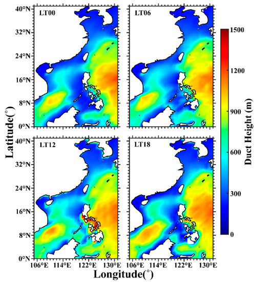
Figure 8.
Distribution of duct altitude at different local times.
3.3. Duct Thickness
Duct thickness is defined as the difference between a duct’s altitude ht and the bottom altitude hb. In Figure 1a, the duct thickness is also called the duct altitude [11]. A composite duct’s thickness is ht1 − hb1 and ht2 − hb2, as shown in Figure 1d.
Figure 9 shows the monthly and seasonal variations in duct thickness. The duct thickness in most continental coastal areas was less than 150 m, which was lower than that over the open sea. The areas where the thickest duct events occurred aligned with the areas where the most duct events occurred. The thickest ducts were mainly concentrated in the Pacific Ocean on the east side of the East China Sea, the Philippines, and Taiwan, and in the South China Sea. Meanwhile, these areas were also where the duct thickness changed most significantly. The variations in duct thickness between spring and summer were the most prominent in the southwest of the South China Sea. In spring, the duct thickness was more than 400 m, whereas it decreased sharply in summer. The Pacific Ocean on the east side of the East China Sea, the Philippines, and Taiwan was another area where strong variations in duct thickness occurred. In autumn, the areas with a duct thickness greater than 300 m in the Pacific Ocean had a trend of moving north and west, whereas they appeared in the sea south of 20°N in winter.
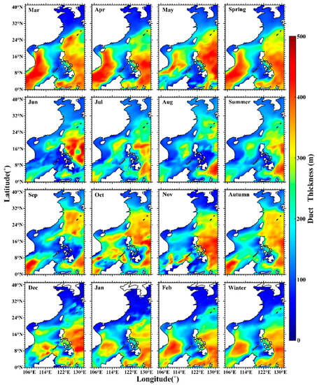
Figure 9.
Distribution of duct thickness, with monthly and seasonal variations.
The distribution of duct thickness across local time variations can be clearly seen in Figure 10. Compared with the distribution of duct altitude, we found that the seas with higher duct altitudes usually have greater duct thickness. The diurnal variation in duct thickness was not obvious, except in minor areas, such as the southwest of the Philippines and the South China Sea. The duct thickness and the coverage range of ducts were larger at LT12 than at other times to the southwest of the Philippines. Furthermore, thicker ducting events occurred in the southwest of the South China Sea at LT18.
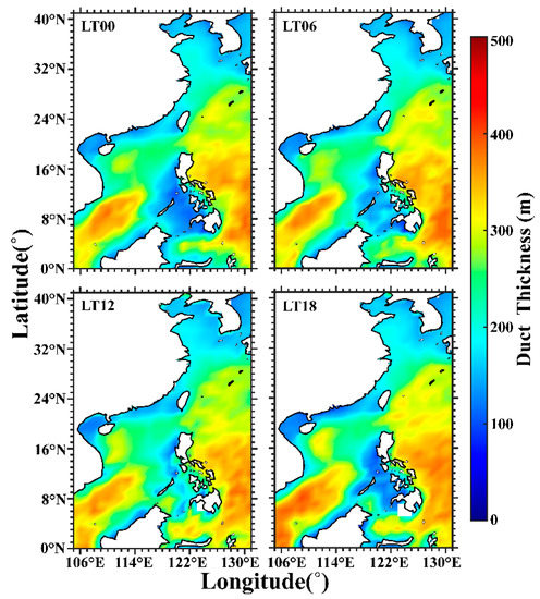
Figure 10.
Distribution of duct thickness at different local times.
3.4. Duct Intensity
Duct intensity refers to the difference in the modified refractivity when the gradient dM/dh < 0; that is, the value of am − as in Figure 1a–c. A composite duct’s intensity is am1 − as1 and am2 − as2. The greater the duct intensity, the greater the influence on electromagnetic wave propagation [1]. The seasonal and monthly variations in the mean duct intensity were statistically obtained, as shown in Figure 11.
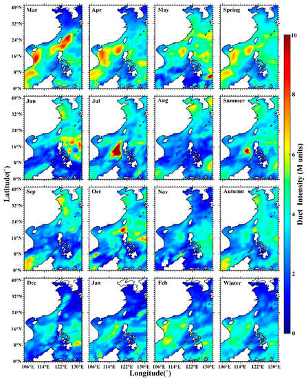
Figure 11.
Distribution of duct intensity, with monthly and seasonal variations.
It can be observed that duct intensity was lower than 10 M-units in the marine areas adjacent to China. In spring, duct intensity was higher than in other seasons. In May, the areas with a duct intensity greater than 4 M-units began to move northward. During this time, the duct intensity began to increase in the Yellow Sea and Bohai Sea. In summer and autumn, the duct intensity was generally weaker than that in spring. The duct intensity over the seas near the Philippines increased significantly in June and July. In winter, the areas with a duct intensity greater than 4 M-units shifted southward and were mainly concentrated in the seas south of 24°N.
Figure 12 shows the local time distributions of duct intensity. The duct intensity was larger at night than during the day. It was more obvious in the northwestern seas of the Philippines, where the intensity was above 6 M-units at LT00 and LT06, while it weakened at LT12 and LT18. The emergence of stronger ducts was related to temperature and humidity gradients, which were mainly affected by solar radiation and sea–land breezes [9,34].
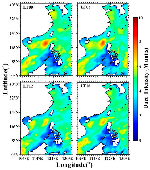
Figure 12.
Distribution of the duct intensity at different local times.
4. Conclusions
Using the 12-year ERA5 data, we statistically analyzed the spatiotemporal distribution characteristics of lower atmospheric ducts in the seas adjacent to China, and the generation mechanisms of ducting events were discussed in this study. The following conclusions can be drawn.
The seasonal and regional distribution features of lower atmospheric ducting events in the seas adjacent to China were obvious, and only minor sea areas had obvious diurnal variations. In May, influenced by the summer monsoon and sea fog, the ducts began to increase in the Yellow Sea and the East China Sea, and gradually shifted to the Bohai Sea. The average duct occurrence rate in these areas was between 20% and 25%; in a few sea areas, it was more than 40%. In June, the duct occurrence rate on the east coast of the Indo-China Peninsula reached the highest value (45.6%) of the whole year. In August, the duct occurrence rate in the Bohai Sea was the maximum for the whole year. However, the duct coverage area in the South China Sea began to decrease sharply in May; especially in autumn, the duct occurrence rate was almost below 10%. The ducts’ altitude in continental coastal seas was obviously lower than that in the open sea. In terms of seasonal variations, duct altitude was the highest in autumn and winter, and lowest in summer. Duct thickness varied between 50 and 450 m, and the areas where the thickest ducts occurred were mainly concentrated in the South China Sea and the Pacific Ocean east of the East China Sea, the Philippines, and Taiwan. Duct intensity was generally lower than 10 M-units, and the areas with a duct intensity greater than 4 M-units began to northward shift in May but shifted south in the winter, and were mainly concentrated in the seas south of 24°N.
Our preliminary statistical results on the climatology of ducts in the seas around China indicate that the variations in the parameters of lower atmospheric ducts were related to factors such as monsoons, tropical cyclones, ocean currents, radiative cooling, sea–land breezes, and other factors. The occurrence of ducts in the Bohai Sea, Yellow Sea, and the East China Sea increased significantly between May and September, which was consistent with the prevalence of summer monsoons. However, between November and March in the following year, due to the influence of winter monsoons, the duct occurrence rate in these areas was sharply reduced. The South China Sea is a tropical ocean with obvious monsoon features and frequent tropical cyclones (typhoons, hurricanes, etc.), which may be the main reason for the seasonal variations in and apparent regional characteristics of the occurrence of ducts in the South China Sea. The ducts’ altitude and thickness in the coastal seas of China were generally lower than those in the open sea, especially in the summer. The higher duct altitude and the greater duct thickness in the Pacific Ocean east of the East China Sea, the Philippines, and Taiwan may be related to the influence of the Japanese Warm Current. We have made only a preliminary investigation into the causes of ducting, and the detailed generation mechanisms need further research.
The local time distribution of the ducts’ parameters in offshore areas of China showed that the diurnal variation in ducts was not obvious, except in minor areas. The main factors of the daily changes in the ducts were roughly divided into the following categories. Firstly, local sea–land breezes had a greater impact on the daily variations in the ducts in coastal seas. Second, strong solar radiation heating led to boundary layer growth and temperature inversions.
Here, we also conducted a statistical analysis of the monthly variations in the number of surface ducts, elevated ducts, and composite ducts. The monthly statistics showed that composite ducting events accounted for less than 1% of the total ducting events, and surface ducts were the main type. The surface ducts had a maximum occurrence rate of 80% and a minimum occurrence rate of 54.6% of all ducting events. Elevated ducts had a maximum occurrence rate of 45.2%. In summer, composite ducts were more likely to appear, especially in July, whereas the number of composite ducting events was lower from October to December.
Supplementary Materials
The following supporting information can be downloaded at: www.mdpi.com/article/10.3390/rs14194864/s1, Map of the adjacent seas of China.
Author Contributions
Conceptualization, Y.Z., Y.L. and C.Z.; methodology, Y.Z.; investigation, Y.Z.; validation, Y.L. and C.Z.; formal analysis, J.Q.; resources, Y.Z. and Y.L.; visualization, J.L.; funding acquisition, Y.L. and C.Z. All authors have read and agreed to the published version of the manuscript.
Funding
This work was supported by a research grant from the China Research Institute of Radiowave Propagation (research on low ionosphere satellite detection), the National Key R&D Program of China (Grant No. 2018YFF01013706), the National Natural Science Foundation of China (NSFC Grant Nos 41574146, 41774162, and 42074187), the National Key R&D Program of China (Grant No. 2018YFC1503506), the foundation of the National Key Laboratory of Electromagnetic Environment (Grant No. 6142403180204), and the Excellent Youth Foundation of Hubei Provincial Natural Science Foundation (Grant No. 2019CFA054).
Data Availability Statement
The study used the dataset from the ECMWF team (https://cds.climate.copernicus.eu/, accessed on 26 September 2021).
Acknowledgments
We acknowledge the use of data from the ECMWF team (https://cds.climate.copernicus.eu/, accessed on 26 September 2021).
Conflicts of Interest
The authors declare no conflict of interest.
References
- Turton, J.D.; Bennets, D.A.; Farmer, S.F.G. An introduction to radio ducting. Meteorol. Mag. 1988, 117, 245–254. [Google Scholar]
- Hitney, H.V.; Richter, J.H.; Pappert, R.A.; Anderson, K.D.; Baumgartner, G.B. Tropo-spheric radio propagation assessment. Proc. IEEE 1985, 73, 265–283. [Google Scholar] [CrossRef]
- Babin, S.M. Surface duct height distributions for Wallops Island, Virginia, 1985–1994. J. Appl. Meteorol. 1996, 35, 86–93. [Google Scholar] [CrossRef]
- Yang, K.; Zhang, Q.; Shi, Y. On analyzing space-time distribution of evaporation duct heig-ht over the global ocean. Acta Oceanol. Sin. 2016, 35, 20–29. [Google Scholar] [CrossRef]
- Von Engeln, A.; Nedoluha, G.; Teixeira, J. An analysis of the frequency and distribution of ducting events in simulated radio occultation measurements based on ECMWF fields. J. Geophys. Res. 2003, 108, D21. [Google Scholar] [CrossRef]
- Ziemba, D.A. Ducting Conditions for Electromagnetic Wave Propagation in Tropical Disturbances from GPS Dropsonde Data. Master’s Thesis, Department of Meteorology, Naval Postgraduate School, Santa Cruz, CA, USA, 2013. [Google Scholar]
- Ko, H.W.; Sari, J.W.; Skura, J.P. Anomalous microwave propagation through atmospheric ducts. Johns Hopkins APL Tech. Dig. 1983, 4, 12–26. [Google Scholar]
- Skura, J.P. Worldwide anomalous refraction and its effects on electromagnetic wave pro-pagation. Johns Hopkins APL Tech. Dig. 1987, 8, 418–425. [Google Scholar]
- Zhu, M.; Atkinson, B.W. Simulated Climatology of Atmospheric Ducts over the Persian Gulf. Bound. Layer Meteorol. 2005, 115, 433–452. [Google Scholar] [CrossRef]
- Patterson, W. Climatology of Marine Atmospheric Refractive Effects: A Compendium of the Integrated Refractive Effects Prediction System (IREPS) Historical Summaries; NOSC Tec-h, Doc.573; Naval Ocean Systems Center: San Diego, CA, USA, 1982; p. 522. [Google Scholar]
- Brooks, I.; Goroch, A.; Rogers, D. Observations of strong surface radar ducts over the Persian Gulf. J. Appl. Meteor. 1999, 38, 1293–1310. [Google Scholar] [CrossRef]
- Mentes, S.; Kaymaz, Z. Investigation of surface duct conditions over Istanbul, Turkey. J. Appl. Meteor. Climatol. 2007, 46, 318–337. [Google Scholar] [CrossRef]
- Basha, G.; Ratnam, M.V.; Manjula, G. Anomalous propagation conditions observed over a tropical station using high-resolution GPS radiosonde observations. Radio Sci. 2013, 48, 42–49. [Google Scholar] [CrossRef]
- Zhao, X.; Wang, D.; Huang, S.X. Statistical estimations of atmospheric duct over the South China Sea and the tropical eastern Indian Ocean. Chin. Sci. Bull. 2013, 58, 2794–2797. [Google Scholar] [CrossRef]
- Cheng, Y.; Zhou, S.; Wang, D.; Lu, Y.; Huang, K.; Yao, J.; You, X. Observed characteristics of atmospheric ducts over the South China Sea in autumn. Chin. J. Oceanol. Limnol. 2016, 34, 619–628. [Google Scholar] [CrossRef]
- Engeln, V.A. Ducting climatology derived from the European Centre for Medium-Range Weather Forecasts global analysis fields. J. Geophys. Res. 2004, 109, 159–172. [Google Scholar] [CrossRef]
- Lopez, P.A. 5-yr 40-km-resolution global climatology of super-refraction for ground-based weather radars. J. Appl. Meteorol. Climatol. 2008, 48, 89–110. [Google Scholar] [CrossRef]
- Sirkova, I. Duct occurrence and characteristics for Bulgarian Black Sea shore derived from ECMWF data-ScienceDirect. J. Atmos. Sol. Terr. Phys. 2015, 135, 107–117. [Google Scholar] [CrossRef]
- Cheng, Y.; Zha, M.; You, Z. Duct climatology over the South China Sea based on European Center for Medium Range Weather Forecast reanalysis data. J. Atmos. Sol. Terr. Phys. 2021, 222, 10–12. [Google Scholar] [CrossRef]
- Hersbach, H. The ERA5 global reanalysis. Q. J. R. Meteorol. Soc. 2020, 146, 1999–2049. [Google Scholar] [CrossRef]
- Kursinski, E.; Hajj, G.; Schofield, J.; Linfield, R.; Hardy, K. Observing Earth’s atmosphere with radio occultation measurements using GPS. J. Geophys. Res. 1997, 102, 429–465. [Google Scholar]
- Kursinski, E.; Hajj, G.; Leroy, S.; Herman, B. The GPS radio occultation technique. Terr. Atmos.Ocean. Sci. 2000, 11, 53–114. [Google Scholar] [CrossRef]
- Bean, B.R.; Dutton, E.J. Radio meteorology. In Technical Report Archive and Image Library; U.S. Government Publishing Office: Washington, DC, USA, 1966. [Google Scholar]
- Almond, T.; Clarke, J. Considerations of the usefulness of the microwave prediction methods on air-to-ground paths. IEEE Proc. Part F 1973, 130, 649–656. [Google Scholar] [CrossRef]
- Babin, S.M.; Rowland, J.R. Observation of a strong surface radar duct using helicopter acquired fine-scale radio refractivity measurements. Geophys. Res. Lett. 1992, 19, 917–920. [Google Scholar] [CrossRef]
- Craig, K.H.; Hayton, T.G. Climatic mapping of refractivity parameters from radiosonde data. In Propagation Assessment in Coastal Environments; AGARDL: Neuilly sur Seine, France, 1995. [Google Scholar]
- Mesnard, F.; Sauvageot, H. Climatology of anomalous propagation radar echoes in a coastal area. J. Appl. Meteorol. Climatol. 2010, 49, 2285–2300. [Google Scholar] [CrossRef]
- Li, P. Study on quality control of radiosonde temperature. Meteorlogical Mon. 2013, 39, 12. [Google Scholar]
- Dyer, S.A.; Dyer, J.S. Cubic-Spline Interpolation: Part 1. IEEE Instrum. Meas. Mag. 2001, 4, 44–46. [Google Scholar] [CrossRef]
- Chen, J. Climatological characteristics of monsoons and tropical cyclone activities over China seas and their influences on hydrological and seasonal structures over the South China Sea. Acta Oceanol. Sin. 1993, 3, 359–377. [Google Scholar]
- Chen, L.; Gao, S.; Kang, S. Statistical analysis on spatial-temporal features of atmospheric ducts over Chinese regional seas. J. Radio Sci. 2009, 24, 702–708. [Google Scholar]
- Zhang, S. Seasonal Variations in the Atmospheric Stratification and the Relations with the Yellow Sea Fog Season. J. Ocean Univ. 2008, 38, 689–698. [Google Scholar]
- Ding, J.; Fei, J.; Huang, X.; Cheng, X. Observational occurrence of tropical cyclone ducts from GPS Dropsonde Data. J. Appl. Meteor. Climatol. 2013, 52, 1221–1236. [Google Scholar] [CrossRef]
- Atkinson, B.W.; Zhu, M. Coastal effects on radar propagation in atmospheric ducting conditions. Meteorol. Appl. 2006, 13, 53–62. [Google Scholar] [CrossRef]
Publisher’s Note: MDPI stays neutral with regard to jurisdictional claims in published maps and institutional affiliations. |
© 2022 by the authors. Licensee MDPI, Basel, Switzerland. This article is an open access article distributed under the terms and conditions of the Creative Commons Attribution (CC BY) license (https://creativecommons.org/licenses/by/4.0/).