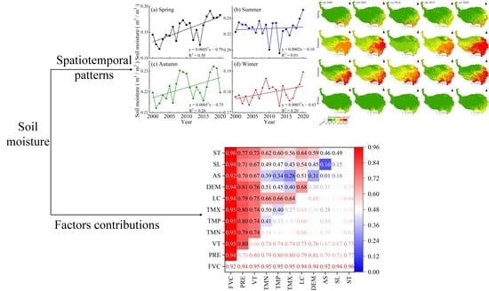
Evaluating the Effects of Climate Change and Human Activities on the Seasonal Trends and Spatial Heterogeneity of Soil Moisture

Abstract

Soil moisture (SM), as a crucial variable in the soil–vegetation–atmosphere continuum, plays an important role in the terrestrial water cycle. Analyzing SM’s variation and driver factors is crucial to maintaining ecosystem diversity on the Tibetan Plateau (TP) and ensuring food security as well as water supply balance in developing countries. Gradual wetting of the soil has been detected and attributed to precipitation in this area. However, there is still a gap in understanding the potential mechanisms. It is unclear whether the greening, glacier melting, and different vegetation degradation caused by asymmetrical climate change and intensified human activities have significantly affected the balance of SM. Here, to test the hypothesis that heterogeneous SM caused by precipitation was subject to temperatures and anthropogenic constraints, GLDAS-2.1 (Global Land Data Assimilation System-2.1) SM products combined with the statistical downscaling and Geographic detectors were applied. The results revealed that: (1) Seasonal SM gradually increased (p < 0.05), while SM deficit frequently appeared with exposure to extreme climates, such as in the summer of 2010 and 2013, and changed into a pattern of precipitation transport to western dry lands in autumn. (2) There was a synergistic reaction between greening and local moisture in autumn. SM was dominated by low temperature (TMN) in winter, warming indirectly regulated SM by exacerbating the thawing of glaciers and permafrost. The spatial coupling between the faster rising rate of TMN and the frozen soil might further aggravate the imbalance of SM. (3) The land cover’s mutual transformation principally affected SM in spring and autumn, and degradation accelerated the loss of SM replenished by precipitation. (4) Land cover responses were different; SM in grassland was less affected by external disturbance, while degraded woodland and shrub performed adaptive feedback under dry environments, SM increased by 0.05 and 0.04 m³/(m³ 10a), respectively. Our research provides a scientific basis for improving hydrological models and developing vegetation restoration strategies for long-term adaptation to TP-changing environments.

1. Introduction

Soil, land cover, and the upper atmosphere are the main components of the land–atmosphere systems [1]. Soil moisture (SM) is a pivotal factor in the soil–vegetation–atmosphere continuum and a carrier of matter and energy cycling in soil systems and plays an important role in the terrestrial water cycle. It not only directly affects hydrological processes and plant growth, such as runoff, infiltration, and evapotranspiration but also indirectly affects regional climate processes [2,3,4]. Some research has shown that the feedback between SM and the atmosphere might amplify temperature and humidity anomalies and enhance the direct effects of SM stress as well [5]. The variability of SM may contribute to 90% of the interannual variability of global land carbon sequestration [6]. Considering the feedback mechanism between soil and atmospheric dryness [7], capturing critical information on regional hydrological responses and providing it to policymakers is significant to achieving China’s commitment to be carbon neutral by 2060 [8,9].

As an important ecological barrier in China, and even in Asia, the Tibetan Plateau (TP) has the largest high-altitude grassland in the world, which is a hotspot of ecosystem diversity [10]. SM controls ecosystem respiration and the occurrences of fire [11]. Vegetation growth depends on surface water availability; SM restrictions not only amplify the mortality risk of plant and herbivores but also lose soil microbial diversity [12,13]. In addition, as the birthplace of major rivers, it is abundant in glacial reservoirs and freshwater resources of alpine lakes, with the largest frozen water storage second only to the polar regions [14]. As a vital freshwater distribution system, the extended water systems of the Yangtze, Yellow, Yarlung Zangbo, and Tarim provide fresh water to nearly 2 billion people in the lower reaches [15]. SM status directly determines the water conservation and runoff recharge in the river source region. SM changes might exacerbate water stress in downstream developing countries. Thus, a balanced SM regime is crucial for maintaining the sustainability of the TP ecosystem and stabilizing the demand for crop irrigation to ensure food security [16].

However, climate change and human activities threaten SM equilibrium. Over the course of its long history, it has experienced faster warming, twice as fast as the global average in the TP [17]. The precipitation patterns have also altered, decreasing in the south and increasing in the northwest [18,19]. The striking socio-economic factors have also increased. Human intervention has led to the serious degradation of grassland-dominated ecosystems and water diversion and expansion of reservoirs [10,20]. Accelerated climate warming, precipitation redistribution, and intensified change in land use have led to the gradual melting of mountain glaciers, permafrost, and snow cover, and to changes in lake distribution and size, and river runoff, remarkably affecting regional hydrological processes. SM responds quickly to external disturbances to the unique geographical environment and fragile ecological conditions [21]. Meanwhile, driven by climate warming and rising regional precipitation, forest lines are expanding to higher elevations, and plenty of green phenomena appeared in the TP from 1982 to 2015, which would have strong positive feedback on the regional hydrological responses, especially in early summer [22]. It indicated that the spatial and seasonal imbalance of SM was gradually increasing. A plentiful number of small-scale observations and experiments have suggested that SM and hydrological characteristics in the alpine region show high spatial variability [23,24]. Better policy decisions require a comprehensive and systematic assessment of the potential mechanisms driving long-term SM variability across the TP. Remotely sensed and reanalysis datasets support the understanding of large-scale hydrological changes, and the selection of reliable SM products is a key step to obtaining robust conclusions [25]. A lot of information has been obtained about the interannual variation in SM dominated by precipitation [26,27,28], while the effects of complex terrains and soil conditions, low temperatures rising faster than high temperatures (asymmetric warming), regional greening, anthropogenic forcing, and extreme climate on SM has largely been dismissed, which may be a misunderstanding of the true states of the SM in the TP.

Based on the long-term reanalysis datasets combined with statistical downscaling, we investigated the trends of 1 km seasonality SM and identified the anomalous yearly SM. Multi-driver factors were selected [29,30,31,32] from three perspectives, such as the biogeographic environment: fractional vegetation coverage (FVC), soil types (ST), vegetation types (VT), elevation (DEM), slope (SL), and aspect (AS), human activities: land covers (LC), and climate: high temperature (TMX), low temperature (TMN), mean temperature (TMP), and precipitation (PRE). A novel mathematical model (geographic detector) was applied to separate their contributions to SM heterogeneity, and comprehensively analyze the vital mechanisms regulating SM changes.

2. Data and Methods

2.1. Study Area

It is located between 26°00′~39°47′N and 73°19′~104°47′E in the TP (Figure 1), which is known as the “roof of the world” or the “third pole” [17], whose three principal climatic types are plateau mountains, subtropical monsoon, and temperate monsoon. Compared with other regions, it is a sensitive area to global climate change. The high temperature (0.06 °C 10 a⁻¹), low temperature (0.15 °C 10 a⁻¹), and mean temperature (0.11 °C 10 a⁻¹) have increased from 2000 to 2020. Precipitation fluctuated strongly in dry environments in 2006 and 2015, with an index of 0.18 mm 10 a⁻¹. It is also the area with the widest distribution of ice, snow, glaciers, and permafrost outside the polar region. The land cover types mainly include broad-leaved forests, coniferous and broad-leaved mixed forests, coniferous forests, shrubs, grassland, desert, and bare land (Figure S1).

2.2. Data

The reanalysis products were generated by GLDAS-2.1 based on the NOAH model driven by the Global Land Data Assimilation System (https://disc.gsfc.nasa.gov/ (accessed on 16 September 2021)), which was a global, high-resolution, land data assimilation system. As many investigations have shown, the GLDAS-2.1 performed better in the spatial patterns and trends of SM in the entire TP [25,33,34,35], compared with other SM products, such as the European Centre for Medium-Range Weather Forecasts (ECMWF) interim reanalysis (ERA-Interim), Essential Climate Variables (ECV) remotely sensed data, and the Modern-Era retrospective analysis for Research and Applications (MERRA). Thus, it was used in this study, starting from January 2000 to December 2020, with a spatial resolution of 0.25° and a temporal resolution of 1 month. It was jointly exploited by the National Aeronautics, Space Administration (NASA) and National Oceanic and Atmospheric Administration (NOAA), and National Centers for Environmental Prediction (NCEP). Furthermore, considering the soil properties of 0–40 cm surface layer (active layer) were more correlated with vegetation characteristics [36], and the roots of regional vegetation were concentrated in soil less than 30 cm [37], we studied 0–40 cm depth SM variations by averaging 0–10 and 10–40 cm profiles SM.

Land cover changes reflect anthropogenic forcing on the earth’s surface, further changing the soil’s physical and chemical properties as well as the precipitation redistribution processes, affecting SM movements [38]. Spatial distribution data of remote sensing monitoring on land use types in China were used, with high classified accuracy (http://www.resdc.cn/DOI (accessed on 25 October 2021)), in six phases, i.e., the years 2000, 2005, 2010, 2015, 2018, and 2020; there were 25 secondary types in this classification system (Table S1), according to land resource and use attributes in the TP, which were merged into 10 classes (

Table 1. Codes of land covers in the TP.

Code	Name	Code	Name	Code	Name
10	Tillage	20	Woodland	22	Shrub
31	High-coverage grassland (with more than 50% coverage)	32	Medium-coverage grassland (with a coverage of 20–50%)	33	Low-coverage grassland (with a coverage of 5–20%)
40	Water	50	Construction land	60	Sand, Gobi, and Bare land
67	Desert

).

One kilometer monthly meteorological variables (TMX, TMN, TMP (TMPs), and PRE) were spatially downscaled from the Climatic Research Unit dataset with the WorldClim dataset. The mean absolute error decreased by 35.4–48.7% for TMPs and by 25.7% for PRE, and the averaged climatology differences between the 0.5′ downscaled and observed data equaled −0.12 to 0.01 °C for TMPs, and −0.5 mm for the annual total PRE (http://www.geodata.cn (accessed on 29 November 2021)), which was reliable to investigate related climate change [39]. In addition, 1 km spatial distributions of the soil types, vegetation types, and elevation data were provided by the Resource and Environmental Science Data Center of the Chinese Academy of Sciences (http://www.resdc.cn/DOI (accessed on 25 October 2021)).

2.3. Methods

2.3.1. Statistical Downscaling GLDAS-2.1 Products

Images with a 25 km resolution might be missing much spatial information [40]; higher spatial resolution is desirable for capturing SM-related hydrological processes. Relevant research suggests that the 100,000 km² area was appropriate for downscaling to a resolution of 1 km [41]. We downscaled GLDAS-2.1 products from 25 km to 1 km through the method proposed by Carlson (1994) [42]. Furthermore, the triangle/trapezoid feature space could be used to monitor SM effectively, and the land surface temperature and vegetation index could reflect well the regional SM. Thus, input variables for statistical downscaling included the 1 km daily TRIMS Land Surface Temperature [43] (Thermal and Reanalysis Integrating Moderate-resolution Spatial-seamless LST; http://data.tpdc.ac.cn (accessed on 23 September 2021); [44]), and the 1 km monthly NDVI (The Normalized Vegetation Index) based on the SPOT/VEGETATION PROBA-V products (http://www.resdc.cn/DOI (accessed on 4 July 2021)). The reliability of LST-NDVI in retrieving SM has also been verified in some regions [38]. Then, the monthly mean LST was calculated from the daily values. Input variables were normalized to eliminate the effects of unit dimension, with the following equations [45]:

$$LS{T}^{*}=\left(LST-LS{T}_{min}\right)/\left(LS{T}_{max}-LS{T}_{min}\right)$$

(1)

$$NDV{I}^{*}=\left(NDVI-NDV{I}_{min}\right)/\left(NDV{I}_{max}-NDV{I}_{min}\right)$$

(2)

where LST and NDVI are the LST and NDVI products, and min and max stand for the corresponding minimum and maximum values, respectively.

LST* and NDVI* were subsequently resampled to a 25 km resolution, consistent with GLDAS-2.1 SM. The relationship between SM and resampling of LST* and NDVI* was established pixel by pixel, as described below [42]:

$$SM={\sum }_{i=0}^n{\sum }_{j=0}^n{a}_{ij}NDV{I}^{*\left(i\right)}LS{T}^{*\left(j\right)}$$

(3)

where $a_{ij}$ represents the independent coefficient; i and j respectively represent the dimension; the 2 or 3 polynomials regression analysis provides a more convincing relationship [38], so n equals 2.

SM, NDVI*, and LST* were known and $a_{ij}$ was estimated through multiple linear regression analysis in MATLAB 2016a software (Mathworks Inc., Natick, MA, USA). Finally, 1 km LST and NDVI data were taken as independent variables to generate high-resolution (1 km) SM mapping. Slope analysis was used for temporal variations.

Hourly SM observation data from the Tibet-Obs (the time-lapse observation dataset of soil temperature and humidity on the TP (2008–2016); http://data.tpdc.ac.cn (accessed on 20 December 2021); [46]) were used to assess and verify SM after downscaling. Only two regional scales in situ observation networks have detected SM at depths of 5, 10, 20, and 40 cm [47]. The cold semiarid climate of the Naqu network and Pali network are presented (Figure 1). These networks provided representative coverage of different climate and surface hydrometeorological conditions on the TP [48], to achieve a more robust evaluation. In addition, previous studies have shown that SM was temporally stable, and site SM data could represent a large area [38,49]. SM in two networks was averaged to maintain the consistent temporal and profile scales as GLDAS-2.1 SM, respectively. The precision was evaluated by determination coefficient (R²) and root mean square error (RMSE).

2.3.2. Contributions of Individual Factor and Their Interactions on SM

In this study, geographic detectors were applied to quantitatively describe the contributions of detection factors to SM, which was a relatively primal spatial statistical model to detect spatial heterogeneity and reveal its driving factors. Furthermore, compared with the linear regression or correlation analysis, this model did not assume that there was a linear or nonlinear response relationship between the two variables. This principle fundamentally ensured that the results were not affected by multicollinearity interference between multiple independent variables. SM was regarded as the dependent variable Y. Potential driving factors were selected as the detection factors X, such as FVC, LC, TMX, TMP, TMN, PRE, ST, VT, DEM, SL, and AS. FVC was estimated by the binary pixel model [50]. The discrete variables were required as input data of geographic detectors; thus, the natural discontinuity method was used to discretize the independent variables and set them into 10 categories (except ST, VT, and LC, which had their own classification system), respectively.

Thus, factor detector, ecological detector, and interactive detector were utilized in this paper. Factor detector could ascertain the effects of potential factors on the spatial heterogeneity of SM. The contribution of X to the spatial heterogeneity of Y could be expressed as q. Moreover, the q value could be simply transformed to satisfy the non-central F distribution and determine the level of significance. The formulas for the factor detector were as follows [51]:

$$q=1-\frac{{\sum }_{h=1}^L{N}_h{\sigma }_h^2}{N{\sigma }^2}=1-\frac{SSW}{SST}$$

(4)

$$W_s=\sum _{h=1}^L{N}_h{\sigma }_h^2, SST=N{\sigma }^2$$

(5)

where h = 1, 2, …, L; L was the stratification of driven factors; $N_h$, N was the layer h, and the number of units in the whole area, respectively; ${\sigma }_h^2$, ${\sigma }^2$ was the variance of the layer h and the whole area, respectively; SSW was the sum of variances within the layer, SST was the total variance of the whole area, respectively. The range of q was [0, 1]. The greater the q was, the stronger the contribution of the driving factor of SM change. An ecological detector was used to detect whether each factor had a significant effect on it. The interaction detector was used to express the degree to which the interaction of any two factors can explain its spatial distribution.

3. Results

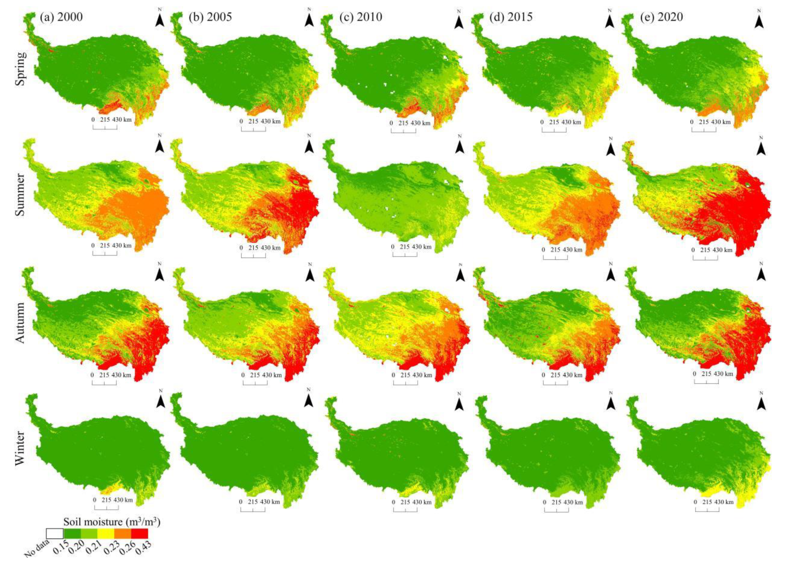
3.1. Spatiotemporal Variations in SM in the TP

These networks provided representative coverage of different climate and surface hydrometeorological conditions on the TP [48]; thus, all stations in Naqu and Pali observation networks were selected, and the SM at the pixel scale of 25 km and 1 km was extracted from images and compared with the measured data, respectively, to verify the accuracy after downscaling. It shows that the R² increased from 0.46 to 0.57, and the RMSE decreased from 0.08 to 0.07 in Figure 2. In general, the dispersion between downscaled SM and field measures was weakened; it showed better performance at a higher spatial resolution.

The annual variation in SM showed an upward trend in the TP overall (Figure S2). Considering merely annual trends may mask seasonal variations. Then, the year was divided into four seasons, which were spring (March to May), summer (June to August), autumn (September to November), and winter (December to February) to capture more spatial and temporal heterogeneity (Figure 3 and Figure 4). The seasonal SM gradually increased over the whole regional scale. It changed fast in spring and autumn, and reached the wettest in summer and winter in 2020, with an increase of 12.41% and 6.76%, respectively, compared with 2000 (relative changes description). However, with the simultaneous occurrence of summer droughts and heat waves in 2010 and 2013, the precipitation was 2.26% and 5.72% less, and the high temperature was 3.60% and 5.19% higher than the multi-year average (Figure 5), which resulted in a serious SM deficit (Figure 3b), SM was 11.71% and 13.67% lower, respectively. Under these circumstances, evapotranspiration appeared to accelerate, and the water supply was insufficient, ultimately leading to an extreme loss of SM. Moreover, SM underwent a sudden continuous growth after 2016 in winter. There was abundant seasonal frozen soil and permafrost in the TP, which accounted for 40% of the total area [52]. Warming processes, permafrost degradation, and glacier and snow melting have been extensively monitored in the TP [17]. Thus, the thawing of frozen soil might be an extra exogenous supplement to promote SM rise (Figure 3d) on account of the higher temperature and lower precipitation in 2017 and 2018 (Figure 5). Seasonal imbalances in SM are expected to intensify as the climate warms, with frequent drier summers and wetter winters.

Spatially, SM showed a spatial pattern that was higher in the southeast and lower in the northwest (Figure S3). Excluding SM anomalies, most areas were becoming wetter, especially in the eastern lower reaches, such as the Sanjiangyuan (the catchment areas of the Yangtze, Yellow, and Lancang rivers), where water resources were abundant. In the vicinity of Tarim Basin, precipitation was scarce, evaporation was intense, and soil was relatively dry. Furthermore, glacier and snow melting and greening further enhanced SM spatial heterogeneity. Such as the northern foothills of the Himalayas, which became significantly redder in the summer of 2020, and patchy local moisture in the southwest and central part of the Plateau in 2015, which was consistent with the distribution of FVC high values (Figure S4). It is worth mentioning the SM deficit in summer, while precipitation reached its peak and most western regions were wetter in autumn (Figure 4 and Figure 5d). This difference might be caused by the decrease in SM, limiting evapotranspiration, regulating atmospheric circulation [53], enhancing the uplift movement of upland and moisture convergence, having positive feedback to precipitation [22], and turning into the mode of water transport to drylands in autumn. In winter, the SM changed from “green” to “yellow” and rose obviously in the alpine regions covered with a large amount of glacial and permafrost, such as the western Kunlun Mountains and the dry areas near the Qaidam Basin.

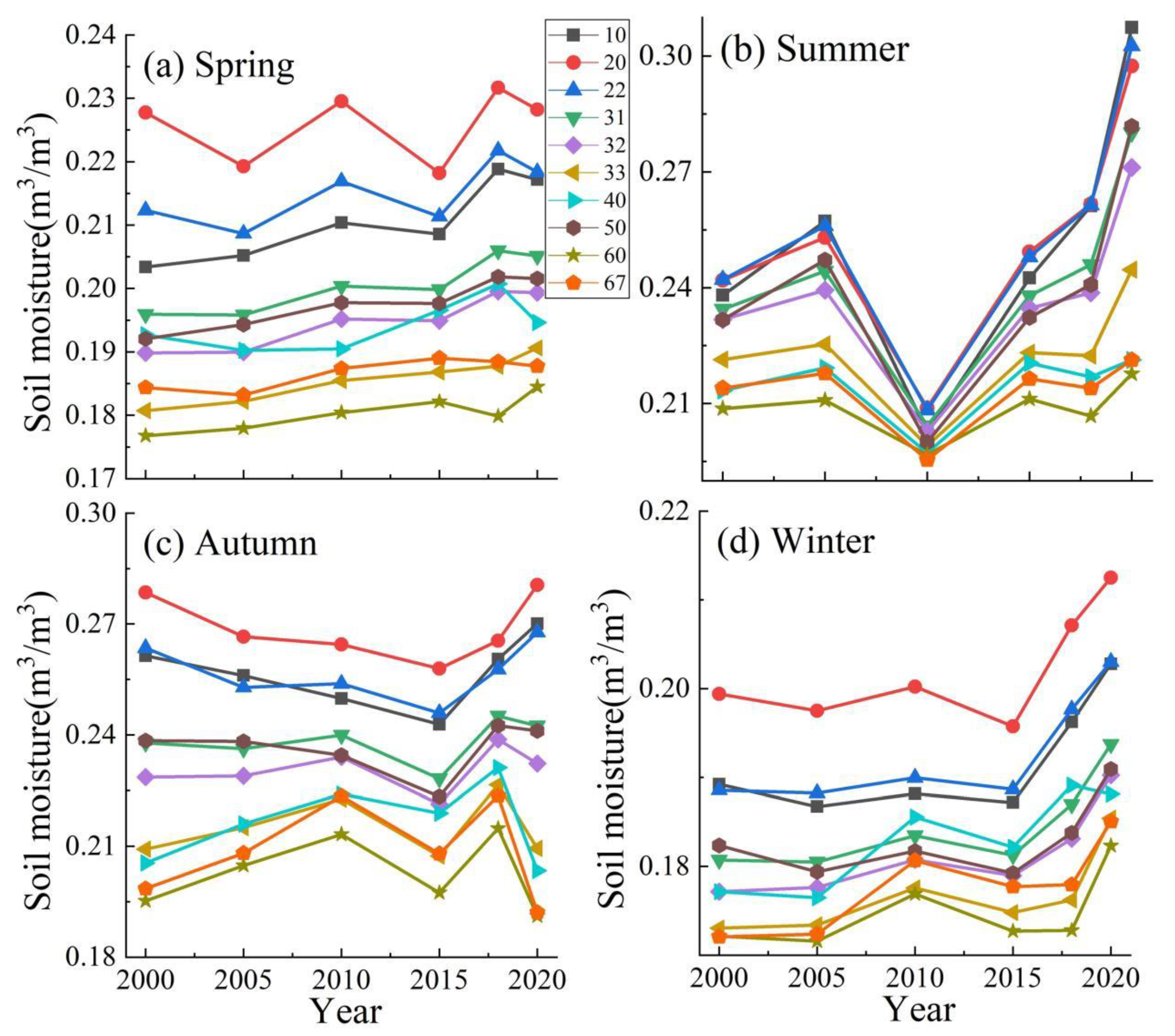
3.2. SM in Different Land Covers

The grassland ecosystem was dominant, accounting for more than 48% on average (

Table 2. The land covers area ratio (%) of the TP from 2000 to 2020.

Land Cover Types	2000	2005	2010	2015	2018	2020
Tillage	1.32	1.30	1.30	1.29	1.29	1.29
Woodland	8.71	8.70	8.71	8.70	8.71	8.70
Shrub	4.47	4.47	4.47	4.47	4.48	4.47
High-coverage grassland	7.81	7.81	7.82	7.81	7.84	7.82
Medium-coverage grassland	18.01	17.99	17.99	17.98	17.97	17.97
Low-coverage grassland	22.64	22.63	22.63	22.62	22.55	22.55
Water	6.22	6.24	6.24	6.26	6.29	6.40
Construction land	0.08	0.09	0.09	0.10	0.10	0.12
Sand gobi and bare land	29.43	29.45	29.45	29.45	29.44	29.35
Desert	1.32	1.32	1.32	1.32	1.32	1.32

). With anthropogenic forcing, land covers changed dramatically. Tillage, shrub, high-coverage grassland, sand, gobi, bare land, and desert dropped sharply, while the amount of water and construction land showed substantial growth (

Table 3. Annual change rate (%/a) of land covers in the TP.

Land Cover Types	2000–2005	2005–2010	2010–2015	2015–2018	2018–2020
Tillage	−0.26	−0.04	−0.10	0.02	−0.13
Woodland	−0.02	0.01	−0.01	0.02	−0.03
Shrub	−0.01	0.03	0.00	0.04	−0.08
High-coverage grassland	0.02	0.01	−0.01	0.12	−0.13
Medium-coverage grassland	−0.02	−0.01	−0.01	−0.02	0.00
Low-coverage grassland	−0.01	0.00	−0.01	−0.09	0.00
Water	0.05	0.00	0.06	0.19	0.81
Construction land	1.31	0.72	2.39	1.56	9.64
Sand gobi and bare land	0.01	0.00	0.00	−0.01	−0.14
Desert	0.01	−0.01	0.00	0.10	−0.15

), especially during the period of 2018–2020. The increase in railway construction might dominate the change in construction land. Due to the unique natural environment and cultural characteristics of the region, social and economic prosperity has promoted the rapid development of tourism, which has become a pillar industry [54].

There were differences in SM among the various types of land cover, and the seasonal SM in woodland persistently remained at a high level (Figure 6). SM in land covers as a whole dropped to the lowest, which meant that extreme drought accelerated transpiration and evaporation, which led to water stress in vegetation roots and increased regional ecosystem vulnerability and irrigation demands [37]. In general, SM in land covers in summer and winter was consistent with the seasonal trends of SM. The interconversion of land covers mainly affected SM in spring and autumn, and partially offset the wetting effects caused by precipitation under degradation. During spring 2018–2020, the soil was gradually moist (Figure 3a) with sufficient precipitation, while the SM of Tillage, woodland, shrub, and grassland decreased (Figure 6a). In addition, land cover responses were different in similar climatic environments. Under degradation, no matter whether the precipitation sharply increased or decreased, SM in high coverage grassland performed at a slightly decreasing rate (slope description), while SM in medium and low coverage grassland was consistent with the precipitation trends (Figure 6a,c). Under restoration conditions, vegetation, such as woodland and shrub, that could effectively increase SM showed higher increasing rates of 0.05 and 0.04 m³/(m³ 10a), respectively, while precipitation was low in spring during 2015–2018 (Figure 5d). Correspondingly, precipitation increased in autumn, and SM increased more swiftly (0.06 m³/(m³ 10a)) in vegetation with better improvement, such as high-coverage grassland (0.12%/a). It is worth noting that in moderate dry conditions, i.e., the autumn of 2018–2020, SM increased in degraded woodland and shrub. Furthermore, woody plants and herbaceous have different strategies to respond to dry conditions [55].

3.3. Attribution of the Spatial Heterogeneity of SM to Climate Change, Human Activities, and Complex Terrain

FVC dominated spatial differences in SM. Although q values of each factor changed in different years, the orders of relative importance remained unchanged (Figure 7). Moreover, PRE, VT, and LC contributed more than 50% in 2020 (Figure 7f). The interaction between FVC and ST contributed the most to SM (Figure 7g). In addition, in terms of SM response to temperatures, TMN was more consistent with its spatial pattern than TMX and TMP. Under the sustained climate and land cover changes, compared with other years, the contributions of FVC, PRE, LC, TMX, TMP, and TMN to SM increased in 2020, which means that the spatial imbalance of SM might gradually intensify.

There were seasonal differences in SM driven by climate. SM spatial heterogeneity was controlled by PRE, except for winter, and it contributed most in autumn. SM was affected by the more intense snow and ice melting and vegetation transpiration, thus being more heterogeneous in summer. In contrast, the autumn PRE was more consistent with spatial matching. TMN was dominant in winter (Figure 8d). The effects of temperature, including TMX, TMN, and TMP, on SM, were weakest in summer and strongest in winter.

4. Discussion

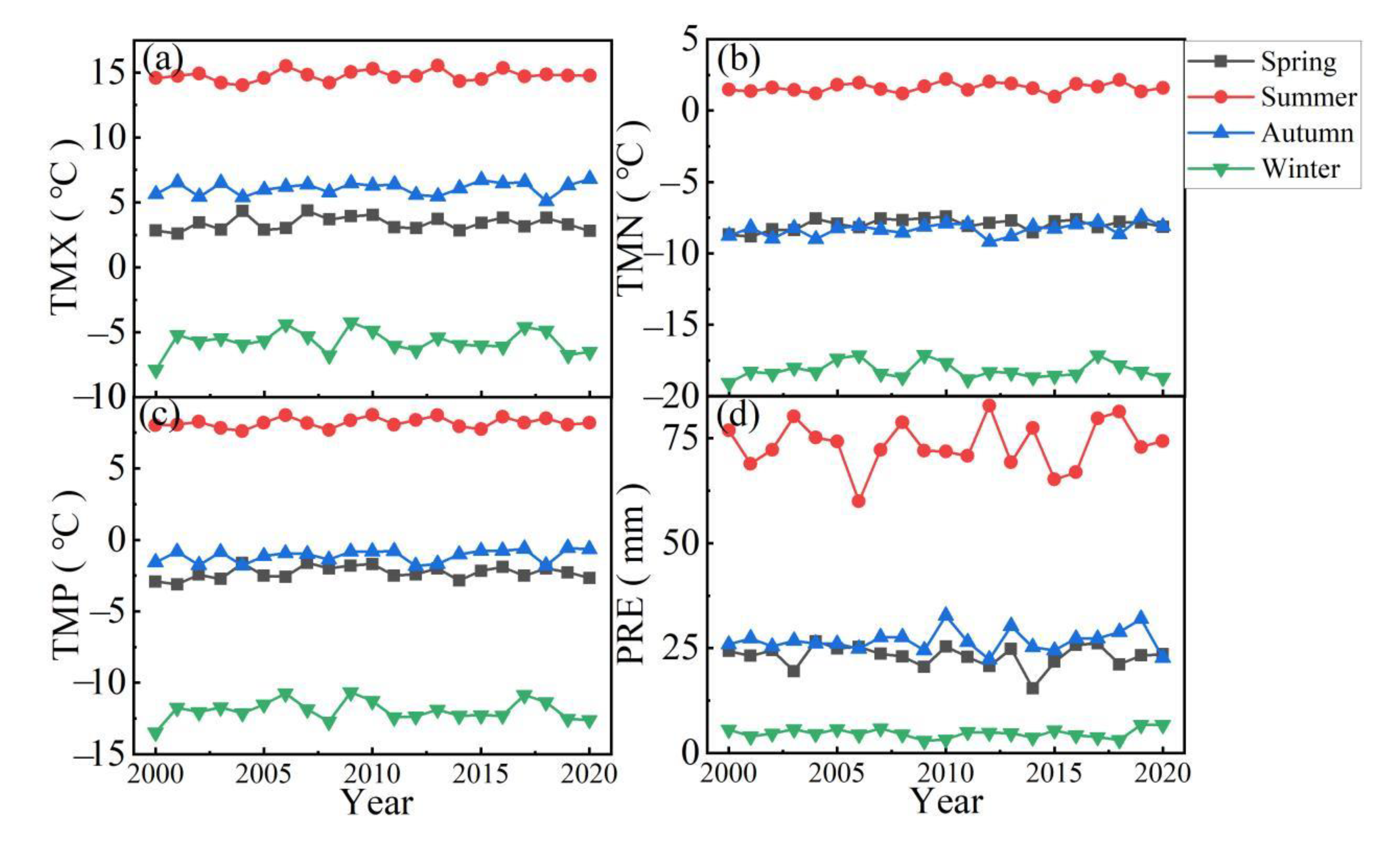
4.1. SM Variation Processes and Response to Climate Change

The wetting trends of SM in the TP showed seasonal thawing characteristics, which was consistent with previous studies [22,25,28,56]. However, SM imbalance was captured at a finer temporal and spatial scale. That is, spatiotemporal heterogeneity was increasing. Similarly, relevant studies have pointed out that an imbalance in freshwater resources in Asia’s water towers is occurring [15]. Regional large-scale asymmetrical warming [57], spatially and seasonally heterogeneous changes in precipitation patterns [18], and frequent human interventions [20] were critical regulatory mechanisms and have altered regional hydrological processes, such as evapotranspiration and surface runoff. The warming rate of TP in winter (0.46 °C/10a) was approximately twice that in summer (0.26 °C/10a) [58]. The regional warming rate increased from south to north [59], accompanied by the asymmetrical warming of TMN and TMX [60]. The growth rate of TMN (0.15 °C/10a) was nearly three times that of TMX (0.06 °C/10a) (Figure 1). Although lower temperatures limited the evapotranspiration process with less precipitation in winter, local dryland wetting was indirectly controlled through the prompt rise of TMN to facilitate the thawing of frozen soil and glaciers; as such, SM appeared to increase in land covers (Figure 6d). The significant influence of temperature on SM was reflected in winter when SM was more sensitive to TMN (Figure 8d), while it would obscure the important role of temperature in the annual cycle [25]. The contributions of spatially coupled patterns of TMN and frozen soil to SM were expected to be more crucial [61]. However, there were trade-offs and large uncertainties. With warming (melting of the cryosphere) and increasing precipitation and anthropogenic forcing, lakes and reservoirs have expanded [20,62,63], and the substantial rising of water cover also provides evidence (Table 2). This might amplify evaporation rates and speed up heat conduction processes [64], and indirectly accelerate SM loss; for example, SM in water cover response was different and decreased in the winter of 2018-2020 (Figure 6d). The feedback mechanisms highlight the urgent necessity to take its related processes into account in earth systems or hydrological models.

Precipitation was the direct source of SM. It increased in the Yangtze River and Yellow River basins while significantly decreasing in the outflow basins such as Yarlung Zangbo River, and its seasonal trends also varied from north to south [15]. It was usually wet in summer and dry in winter (Figure 5d). Notably, changes in westerly winds and Indian monsoons lead to weaker precipitation in the south, and the enhancement of water transport in the west and north of SM in spring and summer [65], directly leads to the seasonal and spatial imbalance of SM.

4.2. Changes in SM Response to Greening

In the process of the interaction between land and atmosphere, vegetation could effectively intercept, block, and consume rainfall [66], as a link to regulate and buffer the water cycle. The state of water absorption of the root system in the shallow layer also affects the dynamic changes in SM [67]. The indirect effects of high temperature and wind speed on the SM were achieved by influencing the plants’ transpiration and respiration. Fractional vegetation coverage was affected by temperature, precipitation, humidity, sunlight, etc. [68]. In that case, it could be used as an integrated indicator to explain why it contributed the most to the SM. However, the positive and negative effects of FVC on SM were not fixed. High FVC slowed down surface rainwater loss, roots promoted its infiltration and prevented SM evaporation [69], while greening enhanced transpiration and water loss by expanding leaf area, which reduced local SM, but SM could be either amplified or reduced through altering precipitation patterns [70]. The autumn leaf senescence was delayed [60], transpiration was restricted along with temperature reduction, and demand for moisture decreased, which highlighted the rainfall interception effects of the vegetation canopy. Thus, the synergistic relationship between enhanced greening and local moisture in autumn could be inferred.

4.3. Changes in SM Associated with Human Activities

The responses of SM to human disturbances emerged in spring and autumn when precipitation and vegetation covers were less. Alpine grassland was the most important ecosystem in the TP [21]. In the past few decades, grassland experienced large-scale degradation on account of overgrazing and human activities [10,37], and land cover changes also provided evidence (Table 3). Degradation was beneficial to heat conduction by altering soil’s physical and chemical properties and aggravated SM deficit [71]. Woodland and shrub ecosystems presented similar characteristics. However, SM might be less affected by alpine grassland degradation [36], which was consistent with the responses of medium and low-coverage grassland. Dynamical changing of SM according to precipitation patterns and hydraulic gradient might be a reason, and could partially offset the SM loss caused by degradation [37]. While high coverage grassland remained a slight vulnerability, accompanied by stronger transpiration and root absorption of higher covers might be the reason [36], transpiration was still a crucial component for water loss in alpine ecosystems [72]. The contradictory results indicated the complex mechanisms of SM movements in different vegetation types and coverage levels, and extensive additional research on SM changes was still needed.

In this paper, uncertainties still exist, due to the limited accuracy of original SM products and system errors in statistical methods, such as the overestimated SM during the thawing period [25,33], and the assumption that scattered land cover had similar climate conditions in the region. The impacts of land cover changes on SM might be mixed with climatic factors. The degree of degradation or restoration, different tree species, along with spatial and soil profile scales also influenced hydrological processes [38].

Having more developed roots, organic matter, and litter layer, enhanced infiltration, reduced runoff, and increased water holding capacity [73], SM in woodland was the highest, which was consistent with previous research [38]. What calls for special attention was that degraded woodland and shrub might have different feedback mechanisms for humid and dry environments, and SM could still be effectively enhanced in a somewhat dry climate (Figure 6c). It might be due to shrubs being less sensitive to environmental stress and even closing their stomata, thus making adaptive adjustments to transpiration to avoid excessive water consumption [74]. However, the adaptability threshold was limited Vegetation would suffer SM stress under extreme droughts (Figure 6b). As global warming intensified, the frequency and intensity of extreme drought continued to increase in the future, which had strong negative impacts on plant physiology and ecology, and irrigation needs [55,74]. The different responses of SM posed significant challenges to the management, adaptation, and stability of TP ecosystems as well as the downstream areas with insufficient water resources. It is imperative that we continue to vigorously promote vegetation restoration, improve and breed dominant species that can adapt to the changing environment in the long term, and develop integrated water resources management strategies to enhance the capacity of China and downstream developing countries to adapt to SM imbalance and ensure a sustainable future for world food.

5. Conclusions

In this study, we used GLDAS-2.1 products in combination with downscaling methods and a geographic detector model to investigate seasonal trends in SM at 1 km resolution over the period 2000–2020, and the relative importance of multiple factors in controlling SM spatial heterogeneity in the TP. First, we discovered that soil gradually became wetter at the annual and seasonal scales. Fractional vegetation coverage and precipitation principally dominated spatial heterogeneity of SM. While the seasonal and spatial imbalance of SM increased with warming and anthropogenic constraints. Greening had a strong feedback effect on SM in autumn. SM deficit in summer enhanced autumn dryland wetness, and land covers degradation reduced SM. Moreover, SM was more sensitive to low temperatures in winter, and asymmetric warming might intensify the trends of soil wetting in permafrost areas, while the resulting dramatic expansion of lakes would cause soil drying. What’s more, herbaceous and woody plants had different feedback mechanisms to dry environments. SM was less affected by a disturbance in grassland, and woodland had a stronger ability to adapt to drought. However, there are still some uncertainties due to the limited accuracy of original SM products and system errors in statistical downscaling. Improving the spatial resolution of remote sensing satellite monitoring SM is an effective technical measure to capture more detailed information about SM-related hydrological processes in the future. In addition, focusing on lesser spatial scales or specific vegetation species might improve our knowledge gap of the key mechanisms of SM movements. Overall, our results might prove useful for reducing the uncertainty of hydrological model simulation and guiding management plans and adaptive restoration strategies.

References

1. Wulfmeyer, V.; Turner, D.D.; Baker, B.; Banta, R.; Behrendt, A.; Bonin, T.; Brewer, W.A.; Buban, M.; Choukulkar, A.; Dumas, E.; et al. A new research approach for observing and characterizing land-atmosphere feedback. Bull. Am. Meteorol. Soc. 2018, 99, 1639–1667. [Google Scholar] [CrossRef]
2. Vereecken, H.; Huisman, J.A.; Pachepsky, Y.; Montzka, C.; van der Kruk, J.; Bogena, H.; Weihermueller, L.; Herbst, M.; Martinez, G.; Vanderborght, J. On the spatio-temporal dynamics of soil moisture at the field scale. J. Hydrol. 2014, 516, 76–96. [Google Scholar] [CrossRef]
3. Wang, C.; Fu, B.; Zhang, L.; Xu, Z. Soil moisture-plant interactions: An ecohydrological review. J. Soils Sediments 2019, 19, 1–9. [Google Scholar] [CrossRef]
4. Yang, J.; Chang, J.; Yao, J.; Wang, Y.; Huang, Q.; Xu, G. Impact of natural climate variability on runoff based on Monte Carlo method. J. Water Clim. Chang. 2019, 10, 344–359. [Google Scholar] [CrossRef]
5. Wehrli, K.; Guillod, B.P.; Hauser, M.; Leclair, M.; Seneviratne, S.I. Identifying key driving processes of major recent heat waves. J. Geophys. Res. Atmos. 2019, 124, 11746–11765. [Google Scholar] [CrossRef]
6. Humphrey, V.; Berg, A.; Ciais, P.; Gentine, P.; Jung, M.; Reichstein, M.; Seneviratne, S.I.; Frankenberg, C. Soil moisture-atmosphere feedback dominates land carbon uptake variability. Nature 2021, 592, 65–69. [Google Scholar] [CrossRef] [PubMed]
7. Zhou, S.; Williams, A.P.; Berg, A.M.; Cook, B.I.; Zhang, Y.; Hagemann, S.; Lorenz, R.; Seneviratne, S.I.; Gentine, P. Land-atmosphere feedbacks exacerbate concurrent soil drought and atmospheric aridity. Proc. Natl. Acad. Sci. USA 2019, 116, 18848–18853. [Google Scholar] [CrossRef] [PubMed]
8. Green, J.K.; Seneviratne, S.I.; Berg, A.M.; Findell, K.L.; Hagemann, S.; Lawrence, D.M.; Gentine, P. Large influence of soil moisture on long-term terrestrial carbon uptake. Nature 2019, 565, 476–479. [Google Scholar] [CrossRef]
9. Zhao, X.; Ma, X.; Chen, B.; Shang, Y.; Song, M. Challenges toward carbon neutrality in China: Strategies and countermeasures. Resour. Conserv. Recycl. 2022, 176, 105959. [Google Scholar] [CrossRef]
10. Zhang, W.; Xue, X.; Peng, F.; You, Q.; Hao, A. Meta-analysis of the effects of grassland degradation on plant and soil properties in the alpine meadows of the Qinghai-Tibetan Plateau. Glob. Eco. Conserv. 2019, 20, e00774. [Google Scholar] [CrossRef]
11. Yan, Z.; Bond-Lamberty, B.; Todd-Brown, K.E.; Bailey, V.L.; Li, S.; Liu, C.; Liu, C. A moisture function of soil heterotrophic respiration that incorporates microscale processes. Nat. Commun. 2018, 9, 2562. [Google Scholar] [CrossRef] [PubMed]
12. Anderegg, W.R.L.; Flint, A.; Huang, C.-Y.; Flint, L.; Berry, J.A.; Davis, F.W.; Sperry, J.S.; Field, C.B. Tree mortality predicted from drought-induced vascular damage. Nat. Geosci. 2015, 8, 367–371. [Google Scholar] [CrossRef]
13. Wu, L.; Zhang, Y.; Guo, X.; Ning, D.; Zhou, X.; Feng, J.; Yuan, M.M.; Liu, S.; Guo, J.; Gao, Z.; et al. Reduction of microbial diversity in grassland soil is driven by long-term climate warming. Nat. Microbiol. 2022, 7, 1054–1062. [Google Scholar] [CrossRef]
14. Immerzeel, W.W.; Lutz, A.F.; Andrade, M.; Bahl, A.; Biemans, H.; Bolch, T.; Hyde, S.; Brumby, S.; Davies, B.J.; Elmore, A.C.; et al. Importance and vulnerability of the world’s water towers. Nature 2020, 577, 364–369. [Google Scholar] [CrossRef] [PubMed]
15. Yao, T.D.; Bolch, T.; Chen, D.L.; Gao, J.; Immerzeel, W.; Piao, S.; Su, F.G.; Thompson, L.; Wada, Y.; Wang, L.; et al. The imbalance of the Asian water tower. Nat. Rev. Earth Environ. 2022, 34, 1–15. [Google Scholar] [CrossRef]
16. Zhou, S.; Williams, A.P.; Lintner, B.R.; Berg, A.M.; Zhang, Y.; Keenan, T.F.; Cook, B.I.; Hagemann, S.; Seneviratne, S.I.; Gentine, P. Soil moisture-atmosphere feedbacks mitigate declining water availability in drylands. Nat. Clim. Chang. 2021, 11, 274. [Google Scholar] [CrossRef]
17. Yao, T.; Xue, Y.; Chen, D.; Chen, F.; Thompson, L.; Cui, P.; Koike, T.; Lau, W.K.M.; Lettenmaier, D.; Mosbrugger, V.; et al. Recent Third Pole’s rapid warming accompanies cryospheric melt and water cycle intensification and interactions between monsoon and environment: Multidisciplinary approach with observations, modeling, and analysis. Bull. Am. Meteorol. Soc. 2019, 100, 423–444. [Google Scholar] [CrossRef]
18. Yao, T.; Thompson, L.; Yang, W.; Yu, W.; Gao, Y.; Guo, X.; Yang, X.; Duan, K.; Zhao, H.; Xu, B.; et al. Different glacier status with atmospheric circulations in Tibetan Plateau and surroundings. Nat. Clim. Chang. 2012, 2, 663–667. [Google Scholar] [CrossRef]
19. Yao, R.; Shi, J. Precipitation differences cause contrast patterns of glacier-melt water supplied discharge of two glacier basins between northern and southern Third Pole. Sci. Bull. 2019, 64, 431–434. [Google Scholar] [CrossRef]
20. Zhan, P.F.; Song, C.Q.; Luo, S.X.; Ke, L.H.; Liu, K.; Chen, T. Investigating different timescales of terrestrial water storage changes in the northeastern Tibetan Plateau. J. Hydrol. 2022, 608, 127608. [Google Scholar] [CrossRef]
21. Pan, T.; Hou, S.; Wu, S.; Liu, Y.; Liu, Y.; Zou, X.; Herzberger, A.; Liu, J. Variation of soil hydraulic properties with alpine grassland degradation in the eastern Tibetan Plateau. Hydrol. Earth Syst. Sci. 2017, 21, 2249–2261. [Google Scholar] [CrossRef]
22. Zhang, W.; Zhou, T.; Zhang, L. Wetting and greening Tibetan Plateau in early summer in recent decades. J. Geophys. Res. Atmos. 2017, 122, 5808–5822. [Google Scholar] [CrossRef]
23. Strudley, M.W.; Green, T.R.; Ascough, J.C., III. Tillage effects on soil hydraulic properties in space and time: State of the science. Soil Tillage Res. 2008, 99, 4–48. [Google Scholar] [CrossRef]
24. Ma, L.; Ahuja, L.R.; Trout, T.J.; Nolan, B.T.; Malone, R.W. Simulating maize yield and biomass with spatial variability of soil field capacity. Agron. J. 2016, 108, 171–184. [Google Scholar] [CrossRef]
25. Zhang, Q.; Fan, K.; Singh, V.P.; Sun, P.; Shi, P. Evaluation of remotely sensed and reanalysis soil moisture against in situ observations on the Himalayan-Tibetan Plateau. J. Geophys. Res. Atmos. 2018, 123, 7132–7148. [Google Scholar] [CrossRef]
26. Zhang, L.; Zeng, Y.; Zhuang, R.; Szabo, B.; Manfreda, S.; Han, Q.; Su, Z. In situ observation-constrained global surface soil moisture using random forest model. Remote Sens. 2021, 13, 4893. [Google Scholar] [CrossRef]
27. Li, G.; Yu, L.; Liu, T.; Jiao, Y.; Yu, J. Modeling potential impacts on regional climate due to land surface changes across Mongolia Plateau. Remote Sens. 2022, 14, 2947. [Google Scholar] [CrossRef]
28. Li, H.; Liu, F.; Zhang, S.; Zhang, C.; Zhang, C.; Ma, W.; Luo, J. Drying-wetting changes of surface soil moisture and the influencing factors in permafrost regions of the Qinghai-Tibet Plateau, China. Remote Sens. 2022, 14, 2915. [Google Scholar] [CrossRef]
29. Guo, L.; Lin, H. Addressing two bottlenecks to advance the understanding of preferential flow in soils. Adv. Agron. 2018, 147, 61–117. [Google Scholar]
30. Liu, Q.; Hao, Y.; Stebler, E.; Tanaka, N.; Zou, C.B. Impact of plant functional types on coherence between precipitation and soil moisture: A wavelet analysis. Geophys. Res. Lett. 2017, 44, 12197–12207. [Google Scholar] [CrossRef]
31. Sterling, S.M.; Ducharne, A.; Polcher, J. The impact of global land-cover change on the terrestrial water cycle. Nat. Clim. Chang. 2013, 3, 385–390. [Google Scholar] [CrossRef]
32. Yang, L.; Wei, W.; Chen, L.; Mo, B. Response of deep soil moisture to land use and afforestation in the semi-arid Loess Plateau, China. J. Hydrol. 2012, 475, 111–122. [Google Scholar] [CrossRef]
33. Yang, S.; Li, R.; Wu, T.; Hu, G.; Xiao, Y.; Du, Y.; Zhu, X.; Ni, J.; Ma, J.; Zhang, Y.; et al. Evaluation of reanalysis soil temperature and soil moisture products in permafrost regions on the Qinghai-Tibetan Plateau. Geoderma 2020, 377, 114583. [Google Scholar] [CrossRef]
34. Bi, H.; Ma, J.; Zheng, W.; Zeng, J. Comparison of soil moisture in GLDAS model simulations and in situ observations over the Tibetan Plateau. J. Geophys. Res. Atmos. 2016, 121, 2658–2678. [Google Scholar] [CrossRef]
35. Chen, Y.; Yang, K.; Qin, J.; Zhao, L.; Tang, W.; Han, M. Evaluation of AMSR-E retrievals and GLDAS simulations against observations of a soil moisture network on the central Tibetan Plateau. J. Geophys. Res. Atmos. 2013, 118, 4466–4475. [Google Scholar] [CrossRef]
36. Zeng, C.; Zhang, F.; Wang, Q.; Chen, Y.; Joswiak, D.R. Impact of alpine meadow degradation on soil hydraulic properties over the Qinghai-Tibetan Plateau. J. Hydrol. 2013, 478, 148–156. [Google Scholar] [CrossRef]
37. Pan, T.; Hou, S.; Liu, Y.; Tan, Q.; Liu, Y.; Gao, X. In fluence of degradation on soil water availability in an alpine swamp meadow on the eastern edge of the Tibetan Plateau. Sci. Total Environ. 2020, 722, 137677. [Google Scholar] [CrossRef] [PubMed]
38. Feng, H.; Liu, Y. Trajectory based detection of forest-change impacts on surface soil moisture at a basin scale Poyang Lake Basin, China. J. Hydrol. 2014, 514, 337–346. [Google Scholar] [CrossRef]
39. Peng, S.Z.; Ding, Y.X.; Liu, W.Z.; Li, Z. 1 km monthly temperature and precipitation dataset for China from 1901 to 2017. Earth Syst. Sci. Data 2019, 11, 1931–1946. [Google Scholar] [CrossRef]
40. Ming, W.T.; Ji, X.; Zhang, M.D.; Li, Y.G.; Liu, C.; Wang, Y.F.; Li, J.Q. A Hybrid triple collocation-deep learning approach for improving soil moisture estimation from satellite and model-Based data. Remote Sens. 2022, 14, 1744. [Google Scholar] [CrossRef]
41. Jia, S.; Zhu, W.; Lu, A.; Yan, T. A statistical spatial downscaling algorithm of TRMM precipitation based on NDVI and DEM in the Qaidam Basin of China. Remote Sens. Environ. 2011, 115, 3069–3079. [Google Scholar] [CrossRef]
42. Carlson, T.N.; Gillies, R.R. A method to make use of thermal infrared temperature and NDVI measurements to infer surface soil water content and fractional vegetation cover. Remote Sens. Rev. 1994, 9, 161–173. [Google Scholar] [CrossRef]
43. Zhang, X.; Zhou, J.; Tang, W.; Ding, L.; Ma, J.; Zhang, X. Daily 1-km All-Weather Land Surface Temperature Dataset for the Chinese Landmass and Its Surrounding Areas (TRIMS LST; 2000–2020); National Tibetan Plateau Data Center: Tibet, China, 2021. [Google Scholar] [CrossRef]
44. Zhang, X.; Zhou, J.; Liang, S.; Wang, D. A practical reanalysis data and thermal infrared remote sensing data merging (RTM) method for reconstruction of a 1-km all-weather land surface temperature. Remote Sens. Environ. 2021, 260, 112437. [Google Scholar] [CrossRef]
45. Chauhan, N.S.; Miller, S.; Ardanuy, P. Spaceborne soil moisture estimation at high resolution: A microwave-optical/IR synergistic approach. Int. J. Remote Sens. 2003, 24, 4599–4622. [Google Scholar] [CrossRef]
46. Su, Z.; Wen, J.; Dente, L.; van der Velde, R.; Wang, L.; Ma, Y.; Yang, K.; Hu, Z. The Tibetan Plateau observatory of plateau scale soil moisture and soil temperature (Tibet-Obs) for quantifying uncertainties in coarse resolution satellite and model products. Hydrol. Earth Syst. Sci. 2011, 15, 2303–2316. [Google Scholar] [CrossRef]
47. Bob, S.; Yang, K. Time-Lapse Observation Dataset of Soil Temperature and Humidity on the Tibetan Plateau (2008–2016); National Tibetan Plateau Data Center: Tibet, China, 2019. [Google Scholar] [CrossRef]
48. Su, Z.; de Rosnay, P.; Wen, J.; Wang, L.; Zeng, Y. Evaluation of ECMWF’s soil moisture analyses using observations on the Tibetan Plateau. J. Geophys. Res. Atmos. 2013, 118, 5304–5318. [Google Scholar] [CrossRef]
49. Loew, A.; Schlenz, F. A dynamic approach for evaluating coarse scale satellite soil moisture products. Hydrol. Earth Syst. Sci. 2011, 15, 75–90. [Google Scholar] [CrossRef]
50. Wang, R.; Yan, F.; Wang, Y. Vegetation growth status and topographic effects in the Pisha Sandstone area of China. Remote Sens. 2020, 12, 2759. [Google Scholar] [CrossRef]
51. Wang, J.; Xu, C. Geodetector: Principle and prospective. Acta Geol. Sin. 2017, 72, 116–134. [Google Scholar]
52. Zou, D.; Zhao, L.; Sheng, Y.; Chen, J.; Hu, G.; Wu, T.; Wu, J.; Xie, C.; Wu, X.; Pang, Q.; et al. A new map of permafrost distribution on the Tibetan Plateau. Cryosphere 2017, 11, 2527–2542. [Google Scholar] [CrossRef] [Green Version]
53. McColl, K.A.; Alemohammad, S.H.; Akbar, R.; Konings, A.G.; Yueh, S.; Entekhabi, D. The global distribution and dynamics of surface soil moisture. Nat. Geosci. 2017, 10, 100–104. [Google Scholar] [CrossRef]
54. Luo, L.; Duan, Q.; Wang, L.; Zhao, W.; Zhuang, Y. Increased human pressures on the alpine ecosystem along the Qinghai-Tibet railway. Reg. Envir. Chang. 2020, 20, 33. [Google Scholar] [CrossRef]
55. Anderegg, W.R.L.; Trugman, A.T.; Bowling, D.R.; Salvucci, G.; Tuttle, S.E. Plant functional traits and climate influence drought intensification and land-atmosphere feedbacks. Proc. Natl. Acad. Sci. USA 2019, 116, 14071–14076. [Google Scholar] [CrossRef] [PubMed]
56. Meng, X.; Li, R.; Luan, L.; Lyu, S.; Zhang, T.; Ao, Y.; Han, B.; Zhao, L.; Ma, Y. Detecting hydrological consistency between soil moisture and precipitation and changes of soil moisture in summer over the Tibetan Plateau. Clim. Dynam. 2018, 51, 4157–4168. [Google Scholar] [CrossRef]
57. Wang, B.; Bao, Q.; Hoskins, B.; Wu, G.X.; Liu, Y.M. Tibetan plateau warming and precipitation changes in East Asia. Geophys. Res. Lett. 2008, 35, l14702. [Google Scholar] [CrossRef]
58. Yu, H.; Luedeling, E.; Xu, J. Winter and spring warming result in delayed spring phenology on the Tibetan Plateau. Proc. Natl. Acad. Sci. USA 2010, 107, 22151–22156. [Google Scholar] [CrossRef]
59. You, Q.L.; Cai, Z.Y.; Pepin, N.; Chen, D.L.; Ahrens, B.; Jiang, Z.H.; Wu, F.Y.; Kang, S.C.; Zhang, R.N.; Wu, T.H.; et al. Warming amplification over the Arctic Pole and Third Pole: Trends, mechanisms and consequences. Earth-Sci. Rev. 2021, 217, 103625. [Google Scholar] [CrossRef]
60. Piao, S.L.; Liu, Q.; Chen, A.P.; Janssens, I.A.; Fu, Y.S.; Dai, J.H.; Liu, L.L.; Lian, X.; Shen, M.G.; Zhu, X.L. Plant phenology and global climate change: Current progresses and challenges. Glob. Chang. Biol. 2019, 25, 1922–1940. [Google Scholar] [CrossRef] [PubMed]
61. Rounce, D.R.; Hock, R.; Shean, D.E. Glacier mass change in high mountain Asia through 2100 using the open-source python glacier evolution model (PyGEM). Front. Earth Sci. 2020, 7, 331. [Google Scholar] [CrossRef]
62. Guo, Y.H.; Zhang, Y.S.; Ma, N.; Xu, J.Q.; Zhang, T. Long-term changes in evaporation over Siling Co Lake on the Tibetan Plateau and its impact on recent rapid lake expansion. Atmos. Res. 2019, 216, 141–150. [Google Scholar] [CrossRef]
63. Brun, F.; Treichler, D.; Shean, D.; Immerzeel, W.W. Limited contribution of glacier mass loss to the recent increase in Tibetan Plateau lake volume. Front. Earth Sci. 2020, 8, 582060. [Google Scholar] [CrossRef]
64. Song, C.; Sheng, Y.; Zhan, S.; Wang, J.; Ke, L.; Liu, K. Impact of amplified evaporation due to lake expansion on the water budget across the inner Tibetan Plateau. Int. J. Climatol. 2020, 40, 2091–2105. [Google Scholar] [CrossRef]
65. Kong, W.W.; Chiang, J.C.H. Southward shift of westerlies intensifies the east asian early summer rainband following El Nino. Geophys. Res. Lett. 2020, 47, e2020GL088631. [Google Scholar] [CrossRef]
66. English, N.B.; Weltzin, J.F.; Fravolini, A.; Thomas, L.; Williams, D.G. The influence of soil texture and vegetation on soil moisture under rainout shelters in a semi-desert grassland. J. Arid Environ. 2005, 63, 324–343. [Google Scholar] [CrossRef]
67. Yang, L.; Chen, L.; Wei, W. Effects of vegetation restoration on the spatial distribution of soil moisture at the hillslope scale in semi-arid regions. Catena 2015, 124, 138–146. [Google Scholar] [CrossRef]
68. Lamchin, M.; Lee, W.-K.; Jeon, S.W.; Wang, S.; Lim, C.H.; Song, C.; Sung, M. Long-term trend and correlation between vegetation greenness and climate variables in Asia based on satellite data. Sci. Total Environ. 2018, 618, 1089–1095. [Google Scholar] [CrossRef]
69. She, D.; Liu, D.; Xia, Y.; Shao, M.A. Modeling effects of land use and vegetation density on soil water dynamics: Implications on water resource management. Water Resour. Manag. 2014, 28, 2063–2076. [Google Scholar] [CrossRef]
70. Piao, S.; Wang, X.; Park, T.; Chen, C.; Lian, X.; He, Y.; Bjerke, J.W.; Chen, A.; Ciais, P.; Tommervik, H.; et al. Characteristics, drivers and feedbacks of global greening. Nat. Rev. Earth Environ. 2020, 1, 14–27. [Google Scholar] [CrossRef]
71. Peng, F.; Xue, X.; You, Q.; Huang, C.; Dong, S.; Liao, J.; Duan, H.; Tsunekawa, A.; Wang, T. Changes of soil properties regulate the soil organic carbon loss with grassland degradation on the Qinghai-Tibet Plateau. Ecol. Indic. 2018, 93, 572–580. [Google Scholar] [CrossRef]
72. Peng, F.; You, Q.; Xue, X.; Guo, J.; Wang, T. Evapotranspiration and its source components change under experimental warming in alpine meadow ecosystem on the Qinghai-Tibet plateau. Ecol. Eng. 2015, 84, 653–659. [Google Scholar] [CrossRef]
73. Neris, J.; Jimenez, C.; Fuentes, J.; Morillas, G.; Tejedor, M. Vegetation and land-use effects on soil properties and water infiltration of Andisols in Tenerife (Canary Islands, Spain). Catena 2012, 98, 55–62. [Google Scholar] [CrossRef]
74. Iqbal, S.; Zha, T.; Jia, X.; Hayat, M.; Qian, D.; Bourque, C.P.A.; Tian, Y.; Bai, Y.; Liu, P.; Yang, R.; et al. Interannual variation in sap flow response in three xeric shrub species to periodic drought. Agric. For. Meteorol. 2021, 297, 108276. [Google Scholar] [CrossRef]
Figure 1. Map of the study area and its climatic conditions and location of the observation sites on the TP: (a) location of the TP in China, (b) map of the TP, (c) Naqu network, (d) Pali network, (e) high temperature, (f) low temperature. (g) mean temperature, (h) precipitation.
Remotesensing 14 04862 g001
Figure 2. Comparison of (a) GLDAS-2.1 products, and (b) downscaled SM with field measures, respectively.
Remotesensing 14 04862 g002
Figure 3. Changes in seasonal SM in the TP from 2000 to 2020, (a) spring, (b) summer, (c) autumn, and (d) winter, respectively. * was the significance of 0.05 level.
Remotesensing 14 04862 g003
Figure 4. Spatial patterns of seasonal SM in the TP from 2000 to 2020, (a) 2000, (b) 2005, (c) 2010, (d) 2015, and (e) 2020, respectively.
Remotesensing 14 04862 g004
Figure 5. Seasonal climate changes in the TP from 2000 to 2020, (a) TMX, (b) TMN, (c) TMP, (d) PRE, respectively.
Remotesensing 14 04862 g005
Figure 6. Seasonal SM variations in different land covers in the TP from 2000 to 2020: (a) spring, (b) summer, (c) autumn, and (d) winter, respectively. The legend numbers correspond to the land cover codes.
Remotesensing 14 04862 g006
Figure 7. Contributions of driving factors and their interactions to spatial distribution of SM from 2000 to 2020: (a) 2000, (b) 2005, (c) 2010, (d) 2015, (e) 2018, (f) 2020, (g) interactions. The numbers indicated the q values. All q values were statistically significant (p < 0.05). Note: VT, ST, DEM, SL, and AS in other years were missing.
Remotesensing 14 04862 g007
Figure 8. Contributions of climatic factors to the spatial distribution of seasonal SM in 2020, (a) spring: (b) summer, (c) autumn, and (d) winter, respectively.
Remotesensing 14 04862 g008