Detection of Carbon Use Efficiency Extremes and Analysis of Their Forming Climatic Conditions on a Global Scale Using a Remote Sensing-Based Model

Abstract

Carbon use efficiency (CUE) represents the proficiency of plants in transforming carbon dioxide (CO₂) into carbon stock in terrestrial ecosystems. CUE extremes represent ecosystems’ extreme proficiency in carbon transformation. Studying CUE extremes and their forming climate conditions is critical for enhancing ecosystem carbon storage. However, the study of CUE extremes and their forming climate conditions on the global scale is still lacking. In this study, we used the results from the daily Boreal Ecosystem Productivity Simulator (BEPS) model to detect the positive and negative CUE extremes and analyze their forming climatic conditions on a global scale. We found grasslands have the largest potential in changing global CUE, with the contribution being approximately 32.4% to positive extremes and 30.2% to negative extremes. Spring in the Northern Hemisphere (MAM) contributed the most (30.5%) to positive CUE extremes, and summer (JJA) contributed the most (29.7%) to negative CUE extremes. The probabilities of gross primary production (GPP) extremes resulted in CUE extremes (>25.0%) being larger than autotrophic respiration (Ra), indicating CUE extremes were mainly controlled by GPP rather than Ra extremes. Positive temperature anomalies (0~1.0 °C) often accompanied negative CUE extreme events, and positive CUE extreme events attended negative temperature anomalies (−1.0~0 °C). Moreover, positive (0~20.0 mm) and negative precipitation (−20.0~0 mm) anomalies often accompanied positive and negative CUE extremes, respectively. These results suggest that cooler and wetter climate conditions could be beneficial to enhance carbon absorptions of terrestrial ecosystems. The study provides new knowledge on proficiency in carbon transformation by terrestrial ecosystems.

1. Introduction

The global terrestrial ecosystem is a carbon sink and could offset a large proportion of anthropogenic CO₂ emissions [1]. Climate change, especially global warming, has affected the carbon cycle in the terrestrial ecosystem [2]. Thus, exploring the influences of climate change on global carbon absorption is essential, especially within the goal of the Paris Agreement’s ambition to keep global warming below 2 °C, with some even considering 1.5 °C targets [3].

Gross primary production (GPP) quantifies carbon uptake by plant photosynthesis, and net primary production (NPP) is the net carbon stored in plants after autotrophic respiration (Ra). Carbon use efficiency (CUE) is defined as the ratio between NPP and GPP, presenting the proficiency of plants in transforming carbon from the atmosphere into plant materials [4]. CUE could also represent the proportion of carbon assimilation assigned to growth and could deeply impact vegetation structure and functioning [5,6]. CUE is a crucial eco-physiological parameter in shaping ecosystem carbon storage [7,8,9]. Thus, increasing CUE is critical for ecosystem management and mitigating global warming. Extreme events indicate the terrestrial ecosystem’s unusual occurrences and episodes [10,11]. CUE extremes represent unusual episodes of the proficiency of carbon transformation in the terrestrial ecosystem. Positive CUE extremes represent ecosystems’ highest proficiency in carbon sequestrations. Conversely, negative CUE extremes represent more CO₂ being released into the atmosphere through Ra. Therefore, promoting positive and preventing negative CUE extremes is critical for enhancing carbon sequestrations in global terrestrial ecosystems. However, many previous studies focused on investigating the pattern and their climate drivers at global and regional scales for CUE. For example, He et al. (2018) used process-based models to investigate the CUE pattern and its linkage with climate factors. Chen et al. (2019) investigated the CUE variations and their climatic controls in China’s terrestrial ecosystems. Additionally, for extreme productivity events, the studies always focus on studying GPP and NEP extremes at global and regional scales [10,11], and there is still a lack of study on the global scale’s positive and negative CUE extremes.

CUE varies across space with plant function types (PFTs) and climate conditions [9,12]. A previous study suggested that grasslands and croplands have higher annual CUE than forests, and the evergreen needle-leaf forest has a larger CUE than other forest types [4]. The spatial pattern of CUE is mainly regulated by temperature and precipitation. Temperature influences the variation of CUE by affecting both GPP and Ra. GPP increases to a temperature optimum and declines afterwards, while Ra increases exponentially with temperature. Positive temperature and solar radiation extremes could induce positive extremes of GPP in China’s terrestrial ecosystems [10]. GPP and Ra are fundamental determinants of CUE, but which dominant CUE extreme and the climate conditions form the global terrestrial ecosystem’s CUE extremes are unclear.

Ecosystem process models are important tools for simulating GPP and NPP on a global scale. Some previous ecosystem models often defined CUE as a constant, such as CASA [13] and FOREST-BGC [14]. However, CUE varies with PFTs and climate conditions [8]; thus, these models are unsuitable for analyzing the CUE extremes and their forming climate conditions. Newly process-based models, which simulate terrestrial ecosystem carbon cycle based on plant major physiological and ecological processes, may offer a new way to study spatial and temporal CUE at the global scale and investigate their forming climate conditions [15,16,17]. The Boreal Ecosystem Productivity Simulator (BEPS) model is driven by remote sensing leaf area index (LAI) and could simulate ecosystem productivity at a global scale and long time series [18]. The BEPS model’s performance is better than prognostic models in simulating productivity in global terrestrial ecosystems [19]. This is because the prognostic models have large uncertainty in the vegetation structural simulation, but satellite remote sensing could monitor vegetation changes on a global scale and provide reliable driven data sources to diagnostic models [19].

In this study, we detected CUE extremes, investigated their linkage with GPP and Ra extremes, and then combined climate data to explore the climate conditions on CUE extreme events based on the BEPS model. The objectives are (i) to compare the extremes of positive and negative CUE and their composition on a global scale, (ii) to investigate the relative contributions of GPP and Ra extremes in the formation of CUE extremes, and (iii) to explore the climate conditions on forming the positive and negative CUE extremes on a global scale during 1982–2016. This study could provide new knowledge on enhancing carbon sequestration and mitigating global warming.

2. Datasets and Methods

2.1. The BEPS Model

The BEPS model’s GPP and NPP simulation results were used in this study. The BEPS is based on the ecosystem process and combines satellite remote sensing data to simulate the global carbon cycle in terrestrial ecosystems [18]. The BEPS model stratifies canopies into sunlit and shaded leaves, simulates photosynthesis by Farquhar’s biogeochemical model [20,21], and then calculates canopy productivity by the sum of sunlit and shaded leaves [18,20]. The BEPS model was originally developed to estimate the carbon budget over Canadian landmass and the NPP in Quebec, but it has been validated with many experimental results and widely used to estimate regional and globe’s terrestrial ecosystem carbon flux, such as in China [10,22], East Asia [23], North America [24], Europe [25], and across the globe [19].

$$GPP=A_{sun}LA{I}_{sun}+A_{shade}LA{I}_{shade},$$

(1)

$$LA{I}_{sun}=2cos\theta \left[1-\exp \left(-\frac{0.5\mathsf{\Omega }LAI}{cos\theta }\right)\right],$$

(2)

$$LA{I}_{shade}=LAI-LA{I}_{sun},$$

(3)

$$NPP=GPP-R_a,$$

(4)

where $A_{sun}$ and $A_{shade}$ are the rate of photosynthesis by sunlit and shaded leaves, respectively. $LA{I}_{sun}$ and $LA{I}_{shade}$ are the LAI of sunlit and shaded leaves, respectively. $\mathsf{\Omega }$ is the foliage clumping index. $\theta$ is the solar zenith angle. $R_a$ is autotrophic respiration.

2.2. Datasets

2.2.1. Global Monthly GPP and NPP Datasets

This study used the same monthly GPP and NPP datasets as in ref. [19]. The GPP and NPP datasets were simulated by the BEPS model, which is driven by remote sensing LAI, clumping index (indicates the foliage’s spatial distribution pattern), and meteorological and soil data. The datasets were validated with an annual global residual land sink (RLS), and the result indicated that the quality of the dataset is pretty good and could be used to analyze the global carbon budget [19].

2.2.2. Climate Data

To analyze the climate conditions for forming CUE extremes, we adopted the monthly temperature, precipitation, and solar radiation from the CRU-NCEP dataset [26]. In this study, all data were resampled into the spatial resolution of 0.5° × 0.5° by the nearest resample method.

2.3. Methods

2.3.1. Calculation of CUE

The CUE was calculated as follows [4]:

$$CUE=\frac{NPP}{GPP}=1-\frac{R_a}{GPP},$$

(5)

where CUE is carbon use efficiency, NPP is net primary production, GPP is gross primary production, and Ra is autotrophic respiration.

To explore the contribution of PFTs and seasonal to positive and negative CUE extremes, we divided the year into four seasons: MAM (March, April, May), JJA (June, July, August), SON (September, October, November), and DJF (December, January, February). We classified the vegetation into eight plant function types: evergreen needleleaf forest (ENF), evergreen broadleaf forest (EBF), deciduous needleleaf forest (DNF), deciduous broadleaf forest (DBF), mixed forests (MF), shrub (SHR), grass (GRA), and cropland (CRO).

We adopted the integrated CUE (iCUE) to analyze the contributions of seasonal and PFTs to CUE extremes. iCUE was calculated by adding the monthly CUE values in the corresponding season or year. Then, the contribution of different seasons and PFTs to CUE extremes was statistically evaluated by weighted area.

2.3.2. Detection of CUE Extremes

The detections of CUE extremes are based on the detrend CUE during the study period. To obtain the detrend CUE, we first estimated the CUE linear trend, then detrend the CUE pixel by pixel from 1982–2016 [10]. The positive CUE extremes are the detrended CUE and were at least 1.5 times the standard deviation higher than the mean value, and the negative CUE extremes are the detrended CUE that were at least 1.5 times the standard deviation lower than the mean value. Similarly, we used the same method to detect GPP and Ra extremes at the pixel level.

2.3.3. The Probabilities of GPP and Ra Extremes Contributed to CUE Extremes

To explore the probabilities of GPP and Ra extremes contributed to CUE extremes, we separately detected GPP, Ra, and CUE extremes at pixel levels. Additionally, we calculated the ratio between the frequencies of concurrence CUE with GPP (Ra) and the frequencies of occurred CUE extremes in each pixel during 1982–2016 [10].

2.3.4. Analysis of the Climate Conditions on the CUE Extremes

We used the partial correlation method to assess the correlations between CUE and climate factors. The method explored the correlations between CUE and individual factors while eliminating the influence of remaining climate factors [10,11]. The datasets were detrended before conducting partial correlation analysis.

To determine the climate conditions in forming CUE extremes, we separately averaged the climate factors’ anomalies in positive and negative CUE extreme events at the pixel level for the four seasons. Additionally, we averaged them with the latitudes to obtain the general climate conditions for CUE extremes.

3. Results

3.1. The Spatial Pattern of the CUE Extremes

The BEPS model simulation results show that the global annual mean CUE was approximately 0.45, ranging from 0.33 to 0.66 (Figure 1a). CUE in the Northern Hemisphere was higher than in the Southern Hemisphere. The highest CUE occurred in some areas of middle–high latitudes in the Northern Hemisphere (>40°N), where the CUE was larger than 0.55. In subtropical regions and the Southern Hemisphere, the CUE was smaller than 0.45. From 1982 to 2016, the spatial pattern of the CUE standard deviations showed that higher CUE regions had higher standard deviations, except for some regions of Australia, where the CUE was smaller than 0.4, but the standard deviation was larger than 0.03 (Figure 1b). These results indicate that the higher CUE regions have more potential to enhance carbon transformation proficiency.

Due to the CUE determined by GPP and Ra, we compared the spatial pattern of GPP and Ra with CUE. The spatial pattern of the annual averaged GPP (Figure 1c) and Ra (Figure 1d) presented a discrepancy from the spatial pattern of CUE. The largest GPP occurred in some areas of tropical regions, where GPP was larger than 2500 gC/m²/y In some regions of eastern North America, European, and Southeast Asia, the GPP was larger than 1500 gC/m²/y but smaller than 2500 gC/m²/y. Other regions’ GPP was smaller than 1500 gC/m²/y. The spatial pattern of Ra (Figure 1d) was similar to GPP. Ra was larger than 1500 gC/m²/y in some tropical areas. In some regions of eastern North America, European, and Southeast Asia, Ra was larger than 600 but smaller than 1500 gC/m²/y. Additionally, in other regions, Ra was smaller than 600 gC/m²/y.

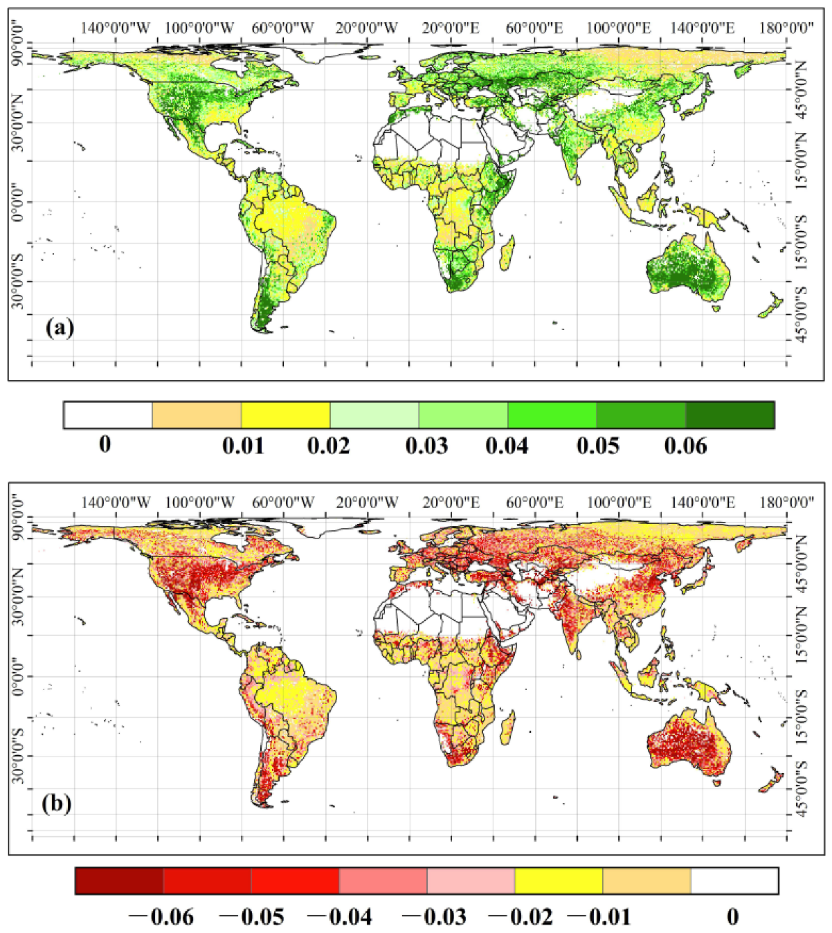
The spatial distribution of the positive CUE extremes was similar to negative CUE extremes (Figure 2), indicating that areas with positive extremes are also prone to negative extremes. Central North America, Europe, and most regions of Australia contributed the largest to positive CUE extremes, with CUE anomalies larger than 0.05. In Northern South America, some areas of Africa, and Southeast Asia, the anomalies of positive CUE were smaller than 0.02 (Figure 2a). Conversely, Central North America, Europe, and most areas of Australia contributed most to negative CUE extremes. The anomalies of negative CUE were smaller than −0.05. In Northern South America, some areas of Africa, and Southeast Asia, the anomalies of positive CUE were larger than −0.02 (Figure 2b).

3.2. The PFTs and Seasonal Contribution to CUE Extremes

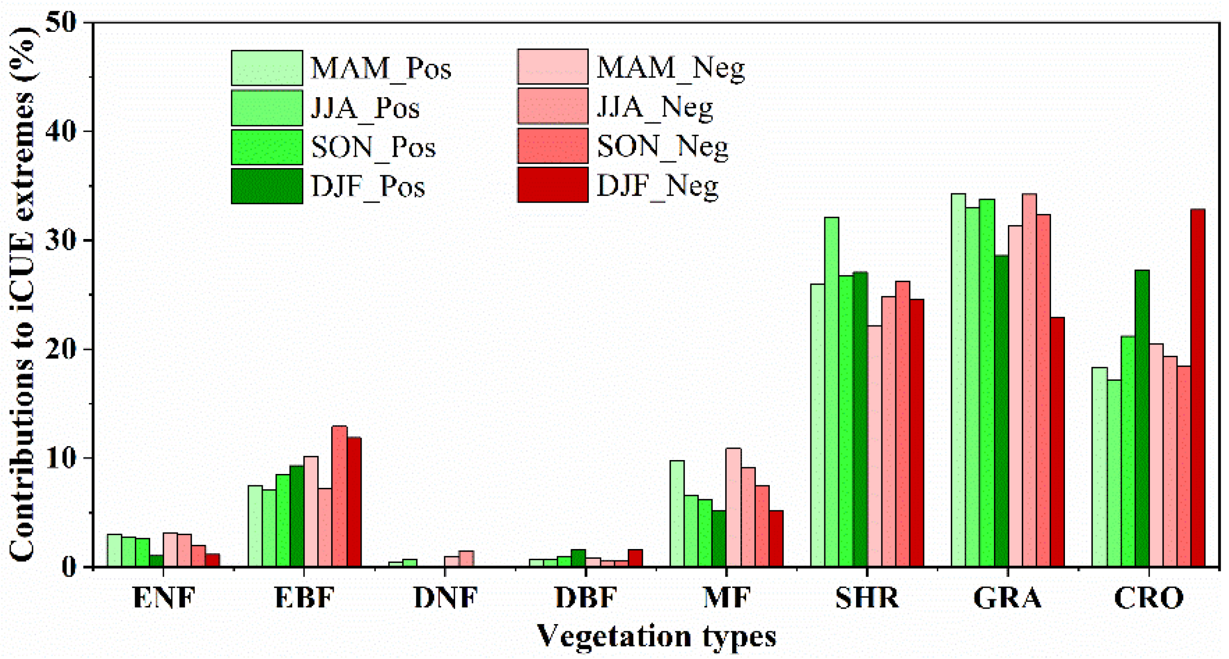
Different PFTs had different contributions to CUE extremes. PFTs also contribute similarly to the positive and negative extremes (Figure 3). Grasslands contributed the largest to CUE extremes, with the contribution being approximately 32.4% to positive extremes and 30.2% to negative extremes, suggesting grassland has a large potential to increase global carbon absorption. Grasslands were followed by shrubs and croplands, contributing approximately 28.0% and 21.0% to positive extremes and 24.5% and 22.8% to negative extremes, respectively. In contrast, forests contributed less to CUE extremes, and the sum of all forests only contributed 17.4% to positive CUE extremes and 22.5% to negative CUE extremes. These results indicate that grasslands have more potential to enhance carbon uptake, and forests have more stability in carbon transformation.

We analyzed the seasonal contributions to CUE extremes (Figure 4). The results indicated that MAM contributed the largest to positive CUE extremes, with a contribution of 30.5%. JJA, SON, and DJF were followed by contributions of 26.2%, 24.4%, and 18.9%. The contribution to negative extremes had some differences from positive extremes. JJA contributed most to negative CUE extremes, with the contribution being 29.7%. Followed by MAM, SON, and DJF, the contributions were 28.4%, 22.4%, and 19.6%. These results suggest that MAM has a larger potential to increase carbon absorption, and JJA is more susceptible to carbon transformation proficiency.

3.3. Correlation of CUE Extremes with GPP and Ra Extremes

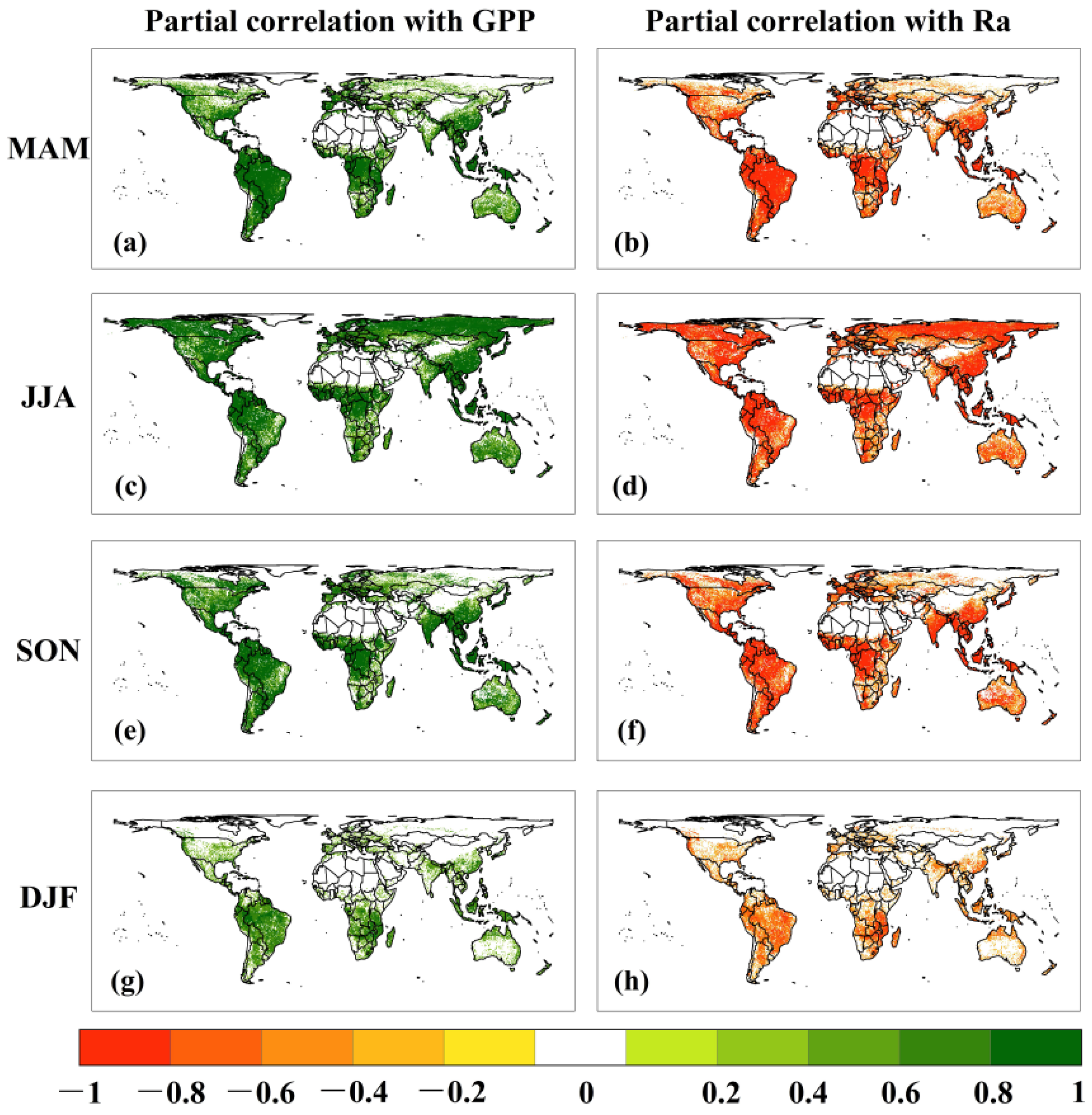
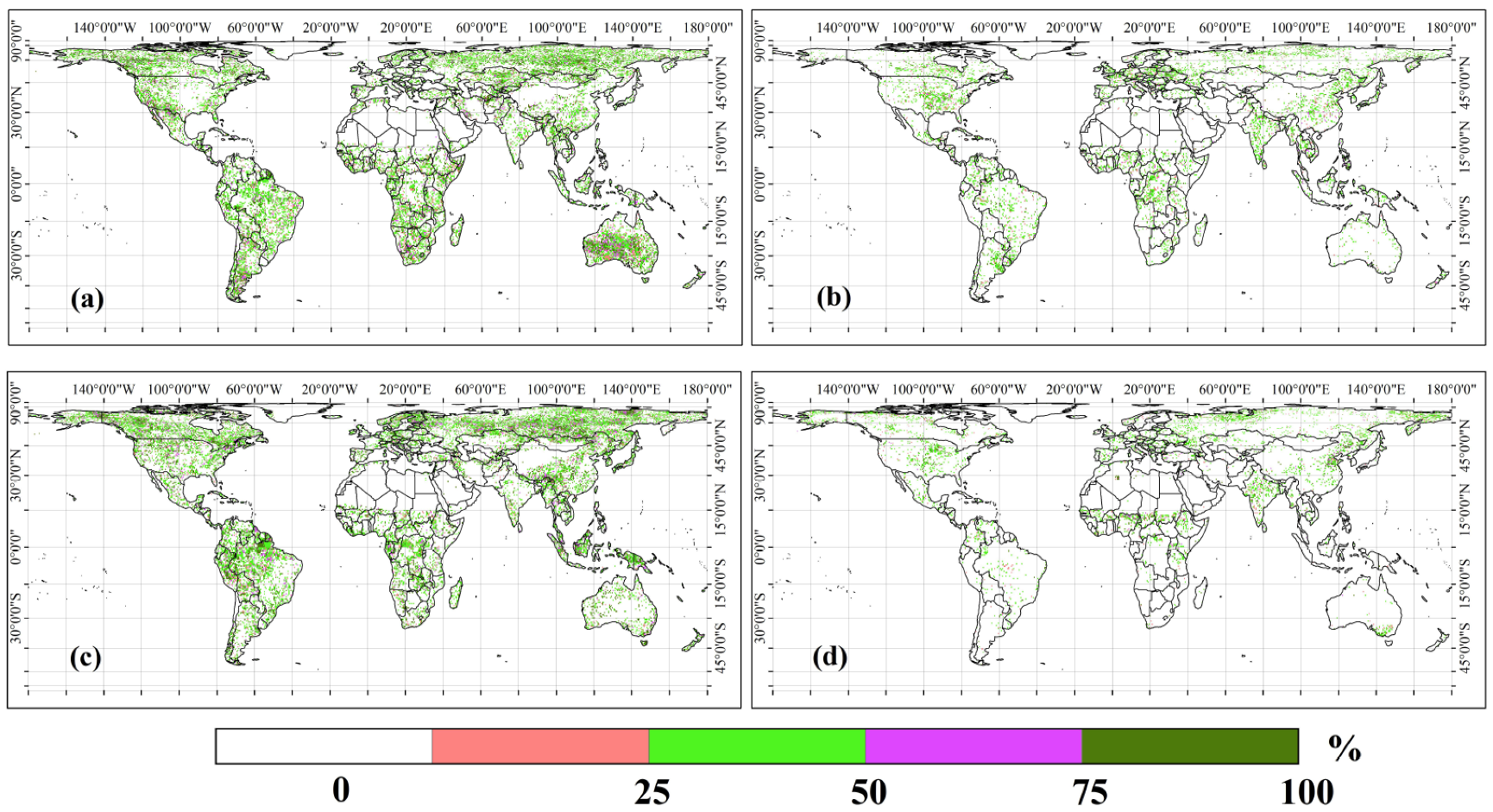
We used the partial correlation method to explore the CUE correlation with GPP and Ra at different seasons (Figure 5). The results indicated there were significant positive correlations between CUE and GPP, with partial correlation coefficients larger than 0.6 in most regions of global. In contrast, the correlation of CUE with Ra was negative in most global areas in different seasons, with the R being smaller than −0.6. Thus, positive CUE extremes may result from positive GPP extremes and negative Ra extremes, and negative CUE extremes may result from negative GPP extremes and positive Ra extremes. Therefore, in this study, we investigated the probabilities of concurrence of positive CUE extremes with positive GPP extremes and negative Ra extremes and negative CUE extremes with negative GPP extremes and positive Ra extremes (Figure 6).

The probabilities of GPP extremes resulted in CUE extremes being larger than Ra (Figure 6). The possibilities of positive GPP extremes resulting in positive CUE extremes were larger than 25% in most areas of the globe (Figure 6a), but the areas of negative Ra extremes that resulted in positive CUE extremes were less and mainly concentrated in some regions of Europe (Figure 6b). Similarly, the probabilities of negative GPP extremes resulting in negative CUE extremes were larger than 25% in most areas of the globe (Figure 6c), but the areas of positive Ra extremes resulted in negative CUE extremes being small (Figure 6d). These results indicated that CUE extremes were mainly controlled by GPP rather than Ra extremes.

3.4. Climate Conditions for CUE Extremes

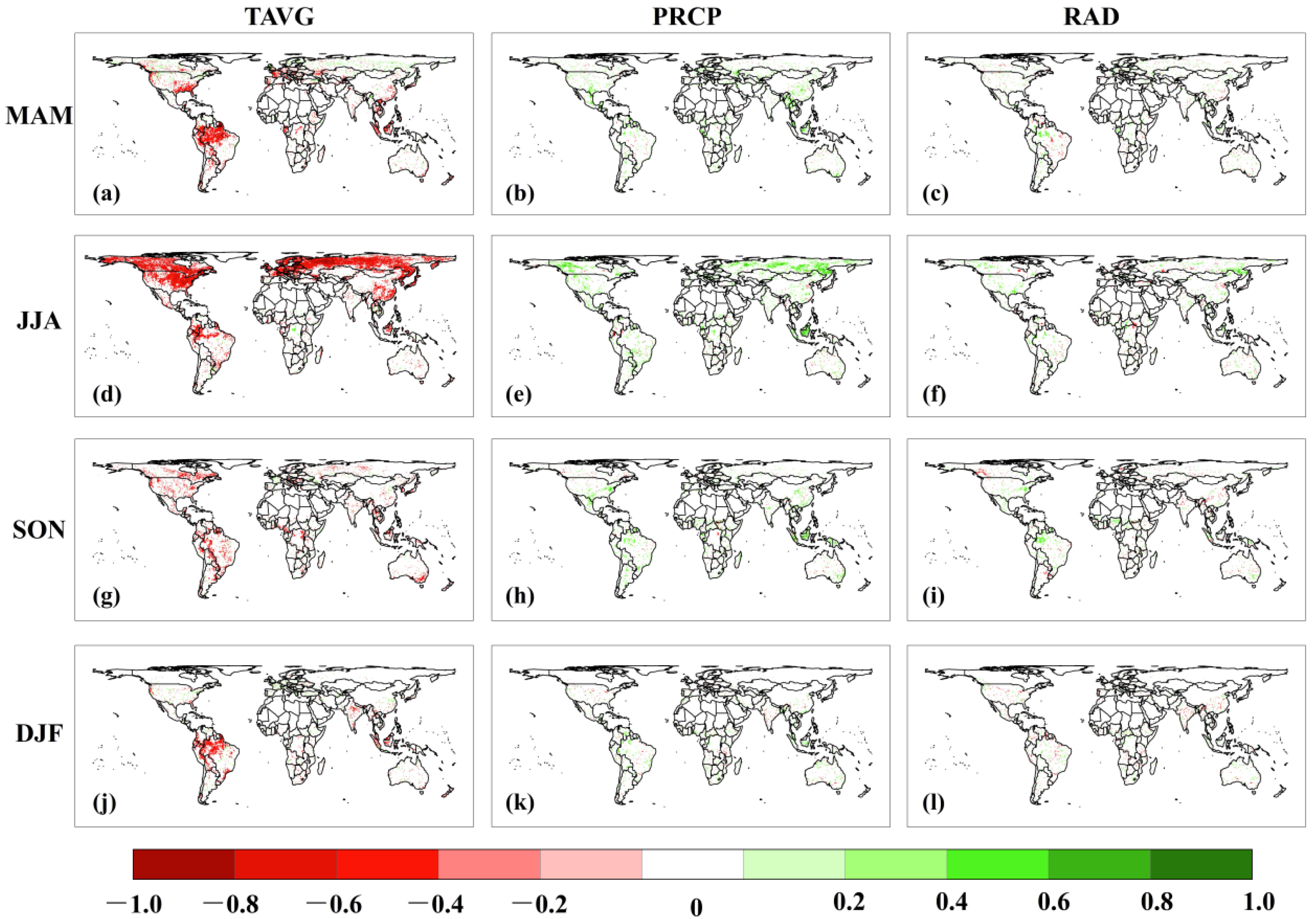
There were no significant correlations between CUE and climatic factors in most areas of the globe. Temperature played a negative role in CUE in some areas of the globe (Figure 7). In MAM and DJF, the correlations of CUE and temperature were negative, with the partial correlation coefficient being smaller than −0.4 in some regions of Southern America. In JJA, the partial correlations between CUE and temperature were smaller than −0.6 in the Northern Hemisphere at high latitudes. The partial correlations between CUE and precipitation were positive in some areas of high latitude in the Northern Hemisphere at JJA, with the partial correlation coefficients larger than 0.4. Additionally, there were no significant correlations in MAM, SON, and DJF. There were no significant correlations between CUE and solar radiations during the four seasons in the global. Thus, we chose temperature and precipitation to analyze the climate conditions of CUE extreme events.

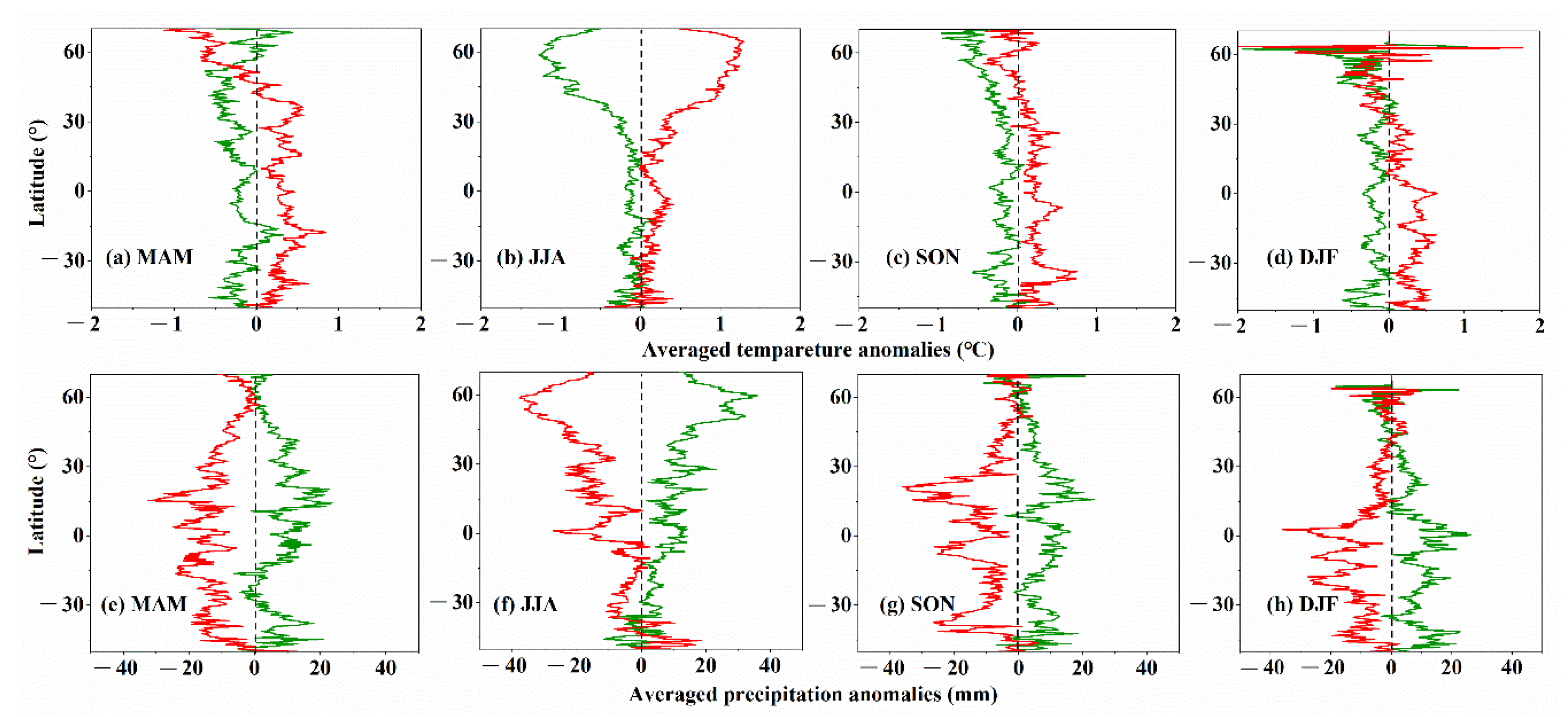
There were opposite temperature anomalies in positive and negative CUE extreme events (Figure 8). Overall, the negative CUE extreme events are often accompanied by positive temperature anomalies, and positive CUE extreme events are attended by negative temperature anomalies in the four seasons. In MAM (Figure 8a), the average temperature anomalies in positive CUE extremes regions ranged from −0.8 °C to 0 °C at different latitudes. Conversely, in most latitude regions, the average temperature anomalies in negative CUE extreme areas ranged from 0 °C to 0.8 °C at different latitudes. In JJA (Figure 8b), the average temperature anomalies were larger than zero in negative CUE extremes and smaller than zero in positive CUE extremes. In particular, at northern middle–high latitudes (>40°N), the temperature anomalies were larger than 1 °C in negative CUE extremes and smaller than −1 °C in positive CUE extremes. In SON (Figure 8c), the average temperature anomalies ranged from −0.5 to 0 °C in positive extremes and 0 to 0.5 °C in negative CUE extremes. In DJF (Figure 8d), there were more obvious temperature anomalies in the Southern Hemisphere than in the Northern Hemisphere, and the average temperature anomalies ranged from −0.5 to 0.5 °C in CUE extremes. These results suggest that warming is harmful to promoting carbon absorption in global terrestrial ecosystems.

Precipitation had opposite performances to temperature in CUE extremes. Positive precipitation anomalies accompany positive CUE, and negative precipitation anomalies attend negative CUE. In MAM (Figure 8e), the precipitation anomalies ranged from 0 to 20 mm in positive CUE extremes and from −20 to 0 mm in the negative CUE extremes. In JJA (Figure 8f), the precipitation anomalies were larger than 20 mm in positive CUE extremes and smaller than −20 mm in negative CUE extremes at middle–high latitudes in the Northern Hemisphere (>40°). In SON (Figure 8g), the precipitation anomalies were larger than 10 mm in positive extremes and smaller than −10 mm in negative extremes at low latitudes (20°N~20°S). In DJF (Figure 8h), the precipitation anomalies in the Southern Hemisphere were larger than in the Northern Hemisphere. The anomalies were larger than 10 mm in positive CUE extremes and smaller than −10 mm in negative CUE extremes. These results indicate that abundant precipitation is critical for increasing the proficiency of carbon absorption in the global terrestrial ecosystems.

4. Discussion

4.1. The Different Contributions of PFTs and Seasonal to CUE Extremes

This study found that middle–high latitudes have higher CUE than low latitudes. This is consistent considering that in high latitude regions, the growing season length is shorter, and vegetations have lower respiratory and higher CUE. Conversely, in low latitude regions where the growing season is more extended, vegetation requires more energy to maintain living tissues, resulting in higher Ra and lower CUE [8].

The study also indicated that grasslands contributed most to CUE extreme events in global terrestrial ecosystems, contributing approximately 32.4% to positive and 30.2% to negative extremes. This is because grasslands are more sensitive to climate change and have higher recovery potential than forest ecosystems, which could alter carbon storage frequently [27,28]. On the other hand, all forest types only contributed 17.4% to positive CUE extremes and 22.5% to negative CUE extremes. This is mainly because forest ecosystems are less sensitive to global climate change and relatively stable in the proficiency of carbon transformation than other PFTs [29].

The results indicated that MAM (spring in the Northern Hemisphere) contributed the largest to positive extremes of CUE, with a contribution of 30.5%. That is because in MAM, vegetation began to grow and sprout, and more carbon fractions could transform to plant tissue to obtain more photosynthesis; thus, intelligent plants could increase their proficiency in converting energy into terrestrial biomass [27]. Additionally, JJA contributed most to negative CUE extremes, with the contribution being 29.7%. JJA is the summer in the Northern Hemisphere, and warming positively increased vegetation productivity in summer in northern and high-latitude regions and negatively increased vegetation productivity in summer in lower latitudes [30]. Thus, global warming, especially in JJA, is unfavorable to promoting global carbon absorption.

4.2. CUE Extremes Were Mainly Controlled by GPP Rather Than Ra Extremes

In this study, we found that the probabilities of GPP extremes resulted in CUE extremes being larger than Ra extremes, with the possibilities of GPP extremes resulting in CUE extremes being larger than 25% in most areas of global terrestrial ecosystems. These results indicated that CUE extremes were mainly controlled by GPP rather than Ra extremes. This is because the GPP is the foundation of the global carbon cycle, representing a natural component to start within any carbon budget [31]. The interannual variations of net carbon uptake in terrestrial are correlated larger with the peak of GPP than respiration [32]. Furthermore, as shown in Figure 1, a larger GPP is always correlated with a larger Ra [33]. Additionally, Ra is only a fraction of GPP, and there is evidence that Ra is closely linked to the supply rate through photosynthesis [34]. Therefore, increasing global plant photosynthesis is essential and beneficial for enhancing the proficiency of carbon sequestrations in ecosystems from the atmosphere. We will investigate how to increase global plant photosynthesis in further work.

4.3. Cooler and Wetter Than the Current Climate Conditions Are Beneficial for Enhancing CUE in Global Terrestrial Ecosystems

This study indicated that CUE extremes are closely related to temperature and precipitation (Figure 7), consistent with the results that a global spatial and temporal pattern of global CUE are strongly associated with temperature and precipitation [35]. We also found that warmer and dryer climate conditions may lead to negative CUE extremes, consistent with the previous study that CUE typically decreases with slight increases in temperature [3]. In some regions of high temperature, Ra is more sensitive to temperature than GPP [8]; therefore, warmer temperatures increase Ra and result in lower CUE in specific areas, such as in some regions in the Northern Hemisphere at high latitude in JJA (Figure 7d). The previous study also indicated that global warming lengthens the growing season and increases ecosystem productivity and biome accumulation. Still, climate warming causes Ra proportionally higher than the increase in GPP [36]. Additionally, higher temperatures might accelerate the process of all biochemical reactions in the plant’s kinetics, while up to high-temperature thresholds beyond which enzymes are inactivated, the CUE will decline [37]. Thus, global warming is not beneficial for enhancing CUE on a global scale.

Precipitation directly influences ecosystem productivity [38]. CUE extremes correlate more with GPP extremes, and abundant precipitation is the foundation of positive GPP extremes [10]. Previous studies indicated that 40~50% of negative GPP extremes resulted from extremely low precipitation [39,40], which agrees with the results of this study. Drought is harmful to vegetation growth [41]. Approximately 40% of GPP extreme events were controlled by precipitation in vegetated areas based on the diagnostic model and eddy covariance data [42]. Although higher CO₂ concentrations can increase GPP, climate change-induced drought, e.g., low soil water availability and heat stress, could reduce GPP at the same time [43]. Therefore, cooler and wetter conditions could enhance carbon absorption on a global scale.

4.4. Uncertainty Analysis

In this study, the BEPS model was used to detect CUE extremes and analyze their forming climate conditions on a global scale. That is because the study requires long time series data, but MODIS GPP and NPP dataset production only started from the year 2000, which is not suitable for analyzing the CUE extremes and comparing them with the result of this study. In addition to the diagnostic model, some prognostic models could be used to simulate global and long-time series productivity datasets, but the prognostic models have large uncertainties in simulating the plant structure and carbon cycle, and the performance of the BEPS model can do a similar or better job than the prognostic models [19]. Therefore, we conducted the analysis based on the BEPS model. Although the BEPS model was validated in previous studies [10,22], there are still some uncertainties. Furthermore, the BEPS model was driven by remote sensing data, which included the land cover change and some human activities on the terrestrial ecosystem [10]; thus, we did not consider the effect of land cover change and human activities on CUE extremes.

In addition, the study only considered the climate conditions on CUE extremes, but other factors, such as soil conditions and nitrogen deposition, could also influence the CUE extremes [37]. Therefore, to better understand CUE extremes and their forming environmental conditions, future studies could consider more environmental factors.

5. Conclusions

This study used the results of BEPS to detect the extremes of positive and negative CUE and analyze their forming climate conditions in global terrestrial ecosystems from 1982 to 2016. We found that the spatial patterns of the anomalies of positive and negative CUE extremes were similar, and grassland has a larger potential to enhance global carbon absorption than forests. MAM contributed most to positive CUE extremes, and JJA contributed most to negative CUE extremes, indicating MAM is the critical season in increasing carbon absorption and needs to take some measurements to decrease Ra in JJA. CUE extremes mostly resulted from GPP extremes rather than Ra extremes, suggesting that increasing global GPP is vital for mitigating global warming. Positive CUE extremes are often accompanied by cooler and wetter than current climate conditions, and warmer and dryer climates could result in negative CUE extremes. This study indicated that cooler temperatures compared to current climate conditions and an abundant water supply are most important to enhance global carbon absorption and mitigate global warming.

References

1. Friedlingstein, P.; O’Sullivan, M.; Jones, M.W.; Andrew, R.M.; Hauck, J.; Olsen, A.; Peters, G.P.; Peters, W.; Pongratz, J.; Sitch, S.; et al. Global Carbon Budget 2020. Earth Syst. Sci. Data 2020, 12, 3269–3340. [Google Scholar] [CrossRef]
2. Wang, M.; Zhao, J.; Wang, S.Q.; Chen, B. Regional Contributions and Climate Attributions to Interannual Variation of Global Net Ecosystems Production by an ECOSYSTEM Processed Model Driven by Remote Sensing Data over the Past 35 Years. Remote Sens. 2022, 14, 3208. [Google Scholar] [CrossRef]
3. Collalti, A.; Trotta, C.; Keenan, T.; Ibrom, A.; Lamberty, B.; Grote, R.; Vicca, S.; Reyer, C.P.O.; Migliavacca, M.; Veroustraete, F.; et al. Thinning Can Reduce Losses in Carbon Use Efficiency and Carbon Stocks in Managed Forests Under Warmer Climate. J. Adv. Model. Earth Syst. 2018, 10, 2427–2452. [Google Scholar] [CrossRef] [PubMed]
4. Chen, Z.; Yu, G. Spatial variations and controls of carbon use efficiency in China’s terrestrial ecosystems. Sci. Rep. 2019, 9, 19516. [Google Scholar] [CrossRef] [PubMed]
5. Li, J.; Wang, G.; Mayes, M.A.; Allison, S.D.; Frey, S.D.; Shi, Z.; Hu, X.M.; Luo, Y.; Melillo, J.M. Reduced carbon use efficiency and increased microbial turnover with soil warming. Glob. Chang. Biol. 2019, 25, 900–910. [Google Scholar] [CrossRef] [PubMed]
6. Geyer, K.M.; Snowman, K.; Grandy, A.S.; Frey, S.D. Microbial carbon use efficiency: Accounting for population, community, and ecosystem-scale controls over the fate of metabolized organic matter. Biogeochemistry 2016, 127, 173–188. [Google Scholar] [CrossRef]
7. Campioli, M.; Vicca, S.; Luyssaert, S. Biomass production effciency controlled by management in temperate and boreal ecosystems. Nat. Genet. 2015, 8, 843–846. [Google Scholar]
8. He, Y.; Piao, S.; Li, X.; Chen, A.; Qin, D. Global patterns of vegetation carbon use efficiency and their climate drivers deduced from MODIS satellite data and process-based models. Agric. For. Meteorol. 2018, 256–257, 150–158. [Google Scholar] [CrossRef]
9. Mathias, J.M.; Trugman, A.T. Climate change impacts plant carbon balance, increasing mean future carbon use efficiency but decreasing total forest extent at dry range edges. Ecol. Lett. 2022, 25, 498–508. [Google Scholar] [CrossRef]
10. Wang, M.M.; Wang, S.Q.; Wang, J.B.; Yan, H.; Mickler, R.A.; Shi, H.; He, H.L.; Huang, M.; Zhou, L. Detection of Positive Gross Primary Production Extremes in Terrestrial Ecosystems of China During 1982-2015 and Analysis of Climate Contribution. J. Geophys. Res.-Biogeosci. 2018, 123, 2807–2823. [Google Scholar] [CrossRef]
11. Wang, M.; Zhao, J.; Wang, S.; Chen, B.; Li, Z. Detection and attribution of positive net ecosystem productivity extremes in China’s terrestrial ecosystems during 2000–2016. Ecol. Indic. 2021, 132, 108323. [Google Scholar] [CrossRef]
12. Drake, J.E.; Furze, M.E.; Tjoelker, M.G.; Carrillo, Y.; Barton, C.V.M.; Pendall, E. Climate warming and tree carbon use efficiency in a whole-tree (13) CO2 tracer study. New Phytol. 2019, 222, 1313–1324. [Google Scholar] [CrossRef] [PubMed]
13. Potter, C.; Randerson, J.T.; Field, C.B. Terrestrial ecosystem production: A process model based on global satellite and surface data. Glob. Biogeochem. Cycles 1993, 7, 811–841. [Google Scholar] [CrossRef]
14. Running, S.W.; Coughlan, J.C. A General-Model of Forest Ecosystem Processes for Regional Applications I. Hydrologic Balance, Canopy Gas-Exchange and Primary Production Processes. Ecol. Model. 1988, 42, 125–154. [Google Scholar] [CrossRef]
15. Piao, S.L.; Liu, Z.; Wang, T.; Peng, S.; Ciais, P.; Huang, M.; Ahlstrom, A.; Burkhart, J.F.; Chevallier, F.; Janssens, I.A.; et al. Weakening temperature control on the interannual variations of spring carbon uptake across northern lands. Nat. Clim. Chang. 2017, 7, 359–363. [Google Scholar] [CrossRef]
16. Liu, D.; Li, Y.; Wang, T.; Peylin, P.; MacBean, N.; Clais, P.; Jia, G.; Ma, M.; Ma, Y.; Shen, M.; et al. Contrasting responses of grassland water and carbon exchanges to climate change between tibetan plateau and inner Mongolia. Agric. For. Meteorol. 2018, 249, 163–175. [Google Scholar] [CrossRef]
17. Wu, D.; Ciais, P.; Viovy, N.; Knapp, A.K.; Wilcox, K.; Bahn, M.; Smith, M.D.; Vicca, S.; Fatichi, S.; Zscheischler, J.; et al. Asymmetric responses of primary productivity to altered precipitation simulated by ecosystem models across three long-term grassland sites. Biogeosci. Discuss. 2018, 15, 3421–3437. [Google Scholar] [CrossRef]
18. Liu, J.; Chen, J.M.; Cihlar, J.; Park, W.M. A process-based boreal ecosystem productivity simulator using remote sensing inputs. Remote Sens. Environ. 1997, 62, 158–175. [Google Scholar] [CrossRef]
19. Chen, J.M.; Ju, W.; Ciais, P.; Viovy, N.; Liu, R.; Liu, Y.; Lu, X. Vegetation structural change since 1981 significantly enhanced the terrestrial carbon sink. Nat. Commun. 2019, 10, 4259. [Google Scholar] [CrossRef]
20. Chen, J.M.; Liu, J.; Cihlar, J.; Goulden, M.L. Daily canopy photosynthesis model through temporal and spatial scaling for remote sensing applications. Ecol. Model. 1999, 124, 99–119. [Google Scholar] [CrossRef]
21. He, S.; Zheng, Z.; Zhu, R. Long-term tea plantation effects on composition and stabilization of soil organic matter in Southwest China. Catena 2021, 199, 105132. [Google Scholar] [CrossRef]
22. He, H.; Wang, S.; Zhang, L.; Wang, J.; Ren, X.; Zhou, L.; Piao, S.; Yan, H.; Ju, W.; Gu, F.; et al. Altered trends in carbon uptake in China’s terrestrial ecosystems under the enhanced summer monsoon and warming hiatus. Nat. Sci. Rev. 2019, 6, 505–514. [Google Scholar]
23. Matsushita, B.; Tamura, M. Integrating remotely sensed data with an ecosystem model to estimate net primary productivity in East Asia. Remote Sens. Environ. 2002, 81, 58–66. [Google Scholar] [CrossRef]
24. Sprintsin, M.; Chen, J.M.; Desai, A.; Gough, C.M. Evaluation of leaf-to-canopy upscaling methodologies against carbon flux data in North America. J. Geophys. Res. Biogeosci. 2012, 117, 313–319. [Google Scholar] [CrossRef]
25. Wang, Q.; Tenhunen, J.; Falge, E.; Bernhofer, C.H.; Granier, A.; Vesala, T. Simulation and scaling of temporal variation in gross primary production for coniferous and deciduous temperate forests. Glob. Chang. Biol. 2004, 10, 37–51. [Google Scholar] [CrossRef]
26. Viovy, N. CRUNCEP Data Set. Available online: Ftp://nacp.ornl.gov/synthesis/2009/frescati/temp/landusechange/original/readme.htm (accessed on 11 August 2018).
27. Du, L.; Gong, F.; Zeng, Y.; Ma, L.; Qiao, C.; Wu, H. Carbon use efficiency of terrestrial ecosystems in desert/grassland biome transition zone: A case in Ningxia province, northwest China. Ecol. Indic. 2021, 120, 106971. [Google Scholar] [CrossRef]
28. Reichstein, M.; Bahn, M.; Ciais, P.; Frank, D.; Mahecha, M.D.; Seneviratne, S.I.; Zscheischler, J.; Beer, C.; Buchmann, N.; Frank, D.C.; et al. Climate extremes and the carbon cycle. Nature 2013, 500, 287–295. [Google Scholar]
29. Frank, D.; Reichstein, M.; Bahn, M.; Thonicke, K.; Frank, D.; Mahecha, M.D.; Smith, P.; van der Velde, M.; Vicca, S.; Babst, F.; et al. Effects of climate extremes on the terrestrial carbon cycle: Concepts, processes and potential future impacts. Glob. Chang. Biol. 2015, 21, 2861–2880. [Google Scholar]
30. Chen, C.; Riley, W.J.; Prentice, I.C.; Keenan, T.F. CO2 fertilization of terrestrial photosynthesis inferred from site to global scales. Proc. Natl. Acad. Sci. USA 2022, 119, e2115627119. [Google Scholar]
31. FatFatichi, S.; Pappas, C.; Zscheischler, J.; Leuzinger, S. Modelling carbon sources and sinks in terrestrial vegetation. New Phytol. 2019, 221, 652–668. [Google Scholar] [CrossRef]
32. Musavi, T.; Migliavacca, M.; Reichstein, M.; Kattge, J.; Wirth, C.; Black, T.A.; Janssens, I.; Knohl, A.; Loustau, D.; Roupsard, O.; et al. Stand age and species richness dampen interannual variation of ecosystem-level photosynthetic capacity. Nat. Ecol. Evol. 2017, 1, 0048. [Google Scholar] [CrossRef] [PubMed]
33. Piao, S.L.; Ciais, P.; Huang, Y.; Shen, Z.H.; Peng, S.S.; Li, J.S.; Zhou, L.P.; Liu, H.Y.; Ma, Y.C.; Ding, Y.H.; et al. The impacts of climate change on water resources and agriculture in China. Nature 2010, 467, 43–51. [Google Scholar] [PubMed]
34. Doughty, C.E.; Santos-Andrade, P.E.; Shenkin, A.; Goldsmith, G.R.; Bentley, L.P.; Blonder, B.; Diaz, S.; Salinas, N.; Enquist, B.J.; Martin, R.E.; et al. Tropical forest leaves may darken in response to climate change. Nat. Ecol. Evol. 2018, 2, 1918–1924. [Google Scholar] [CrossRef] [PubMed]
35. Zhang, Y.; Yu, G.; Yang, J.; Wimberly, M.C.; Zhang, X.; Tao, J.; Jiang, Y.; Zhu, J. Climate-driven global changes in carbon use efficiency. Ecol. Biogeogr. 2013, 23, 144–155. [Google Scholar]
36. Dietze, M.C.; Sala, A.; Carbone, M.S.; Czimczik, C.I.; Mantooth, J.A.; Richardson, A.D.; Vargas, R. Nonstructural carbon in woody plants. Annu. Rev. Plant Biol. 2014, 65, 667–687. [Google Scholar]
37. Collalti, A.; Prentice, I.C. Is NPP proportional to GPP? Waring’s hypothesis 20 years on. Tree Physiol. 2019, 39, 1473–1483. [Google Scholar]
38. Fung, E.; Imbach, P.; Corrales, L.; Vilchez, S.; Zamora, N.; Argotty, F.; Hannah, L.; Ramos, Z. Mapping conservation priorities and connectivity pathways under climate change for tropical ecosystems. Clim. Chang. 2017, 141, 77–92. [Google Scholar]
39. Chen, W.Z.; Zhu, D.; Huang, C.J.; Ciais, P.; Yao, Y.T.; Friedlingstein, P.; Sitch, S.; Haverd, V.; Jain, A.K.; Kato, E.; et al. Negative extreme events in gross primary productivity and their drivers in China during the past three decades. Agric. For. Meteorol. 2019, 275, 47–58. [Google Scholar] [CrossRef]
40. Zscheischler, J.; Reichstein, M.; Harmeling, S.; Rammig, A.; Tomelleri, E.; Mahecha, M.D. Extreme events in gross primary production: A characterization across continents. Biogeosciences 2014, 11, 2909–2924. [Google Scholar] [CrossRef] [Green Version]
41. Wang, M.; Wang, S.; Zhao, J.; Ju, W.; Hao, Z. Global positive gross primary productivity extremes and climate contributions during 1982–2016. Sci. Total Environ. 2021, 774, 145703. [Google Scholar]
42. Beer, C.; Reichstein, M.; Tommelleri, E.; Ciais, P.; Jung, M.; Carvalhais, N.; Rodenbeck, C.; Arain, A.; Baldocchi, D.; Bonan, G.; et al. Terrestrial gross carbon dioxide uptake: Global distribution and covariation with climate. Science 2010, 329, 834–838. [Google Scholar] [PubMed]
43. Xu, C.; McDowell, N.G.; Fisher, R.A.; Wei, L.; Sevanto, S.; Christoffersen, B.O.; Weng, E.; Middleton, R.S. Increasing impacts of extreme droughts on vegetation productivity under climate change. Nat. Clim. Chang. 2019, 9, 948–953. [Google Scholar] [CrossRef] [Green Version]
Figure 1. The spatial pattern of the (a) annual averaged CUE, (b) standard deviations of CUE, (c) GPP, and (d) Ra during 1982–2016.
Remotesensing 14 04873 g001
Figure 2. Spatial pattern of the (a) positive and (b) negative CUE extremes.
Remotesensing 14 04873 g002
Figure 3. The contribution of vegetation types to CUE extremes. “MAM” contains the month of March, April, May; “JJA” contains the month of June, July, and August; “SON” contains the month of September, October, and November; “DJF” contains the month of December, January, February. “Pos” represent the positive extremes, and “Neg” represent negative CUE extremes. “ENF” is evergreen needleleaf forest, “EBF” is evergreen broadleaf forest, “DNF” is deciduous needleleaf forest, “DBF” is deciduous broadleaf forest, “MF” is mixed forest, “SHR” is a shrub, “GRA” is grass, and “CRO” is cropland.
Remotesensing 14 04873 g003
Figure 4. The seasonal contribution to CUE extremes. “MAM” contains the month of March, April, and May; “JJA” contains the month of June, July, and August; “SON” contains the month of September, October, and November; “DJF” contains the month of December, January, and February.
Remotesensing 14 04873 g004
Figure 5. Spatial pattern of the partial correlation coefficients between CUE with GPP and Ra in (a,b) MAM, (c,d) JJA, (e,f) SON, and (g,h) DJF. “MAM” contains the month of March, April, and May; “JJA” contains the month of June, July, and August; “SON” contains the month of September, October, and November; “DJF” contains the month of December, January, and February.
Remotesensing 14 04873 g005
Figure 6. Spatial distribution of the probabilities of concurrence positive extremes of CUE with (a) positive extremes of GPP and (b) negative extremes of Ra. Negative CUE extremes with (c) negative extremes of GPP and (d) positive extremes of Ra.
Remotesensing 14 04873 g006
Figure 7. Spatial pattern of the partial correlation coefficients between CUE and TAVG, PRCP, and RAD in (ac) MAM, (df) JJA, (gi) SON, and (jl) DJF. Shown are significant correlations (p < 0.01). “MAM” contains the month of March, April, and May; “JJA” contains the month of June, July, and August; “SON” contains the month of September, October, and November; “DJF” contains the month of December, January, and February.
Remotesensing 14 04873 g007
Figure 8. The averaged (ad) temperature and (eh) precipitation anomalies in positive (green line) and negative (red line) CUE extremes pixels at different latitudes in the four seasons. “MAM” contains the month of March, April, and May; “JJA” contains the month of June, July, and August; “SON” contains the month of September, October, and November; “DJF” contains the month of December, January, and February.
Remotesensing 14 04873 g008
Publisher’s Note: MDPI stays neutral with regard to jurisdictional claims in published maps and institutional affiliations.