
BSC-Net: Background Suppression Algorithm for Stray Lights in Star Images


Abstract

1. Introduction
1.1. Literature Review
1.2. Imaging Features of Star Images
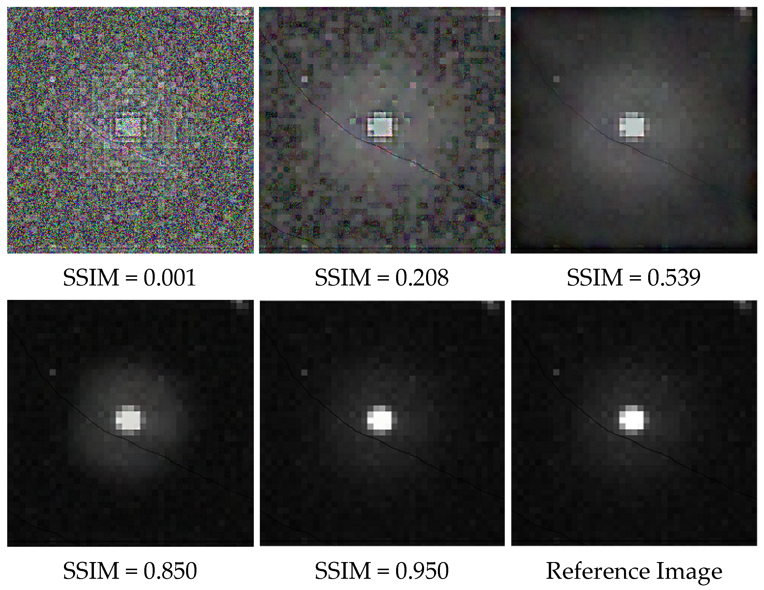
1.3. SSIM and Peak Signal-to-Noise Ratio (PSNR)
2. Methods
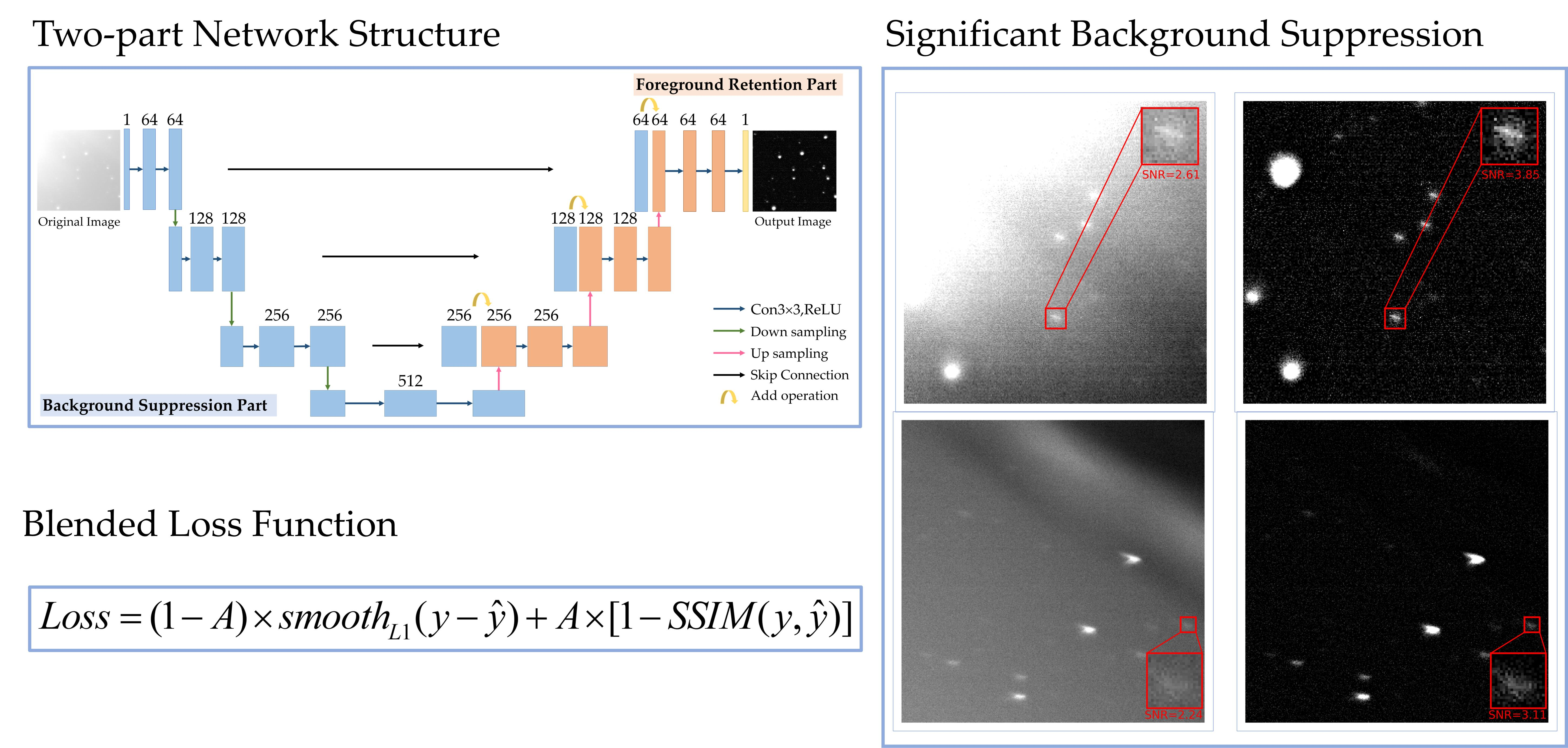
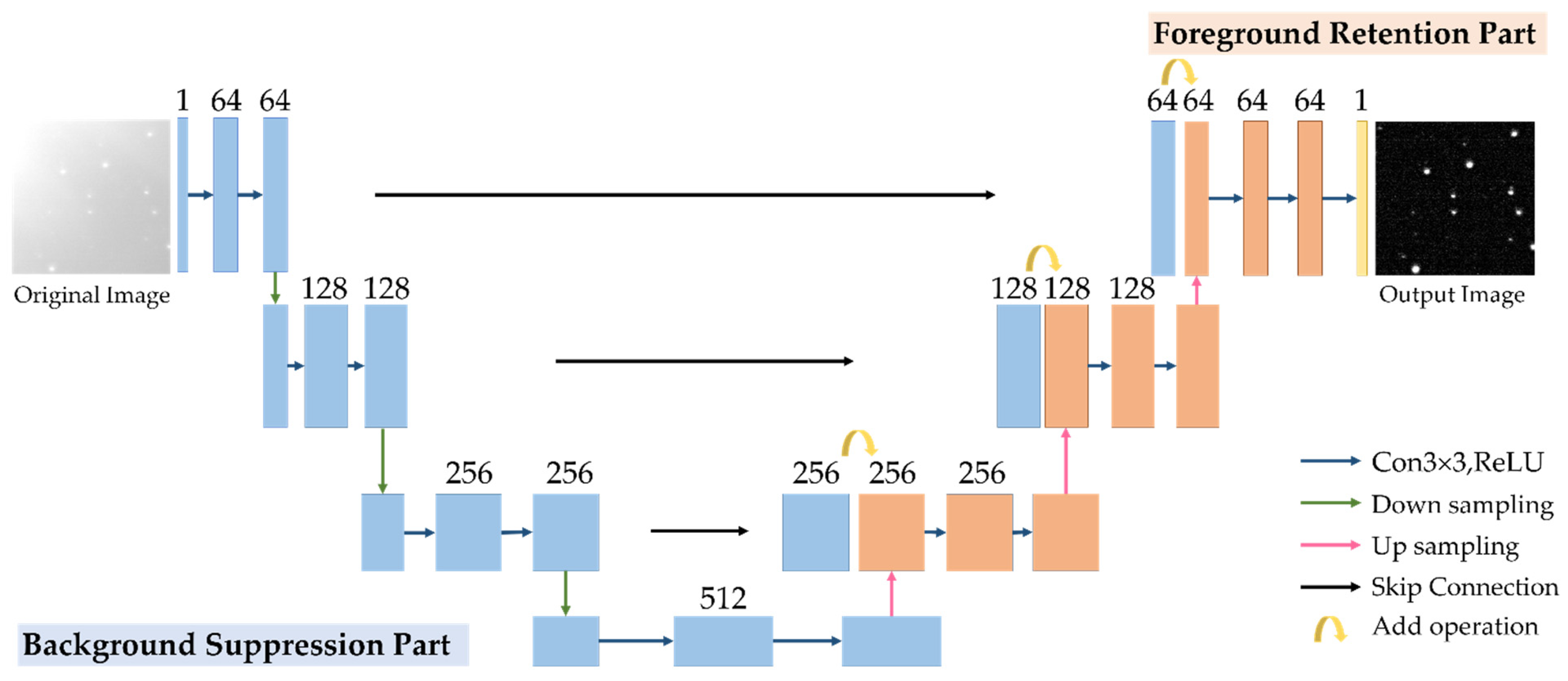
2.1. Network Structure of BSC-Net
2.1.1. Background Suppression Part
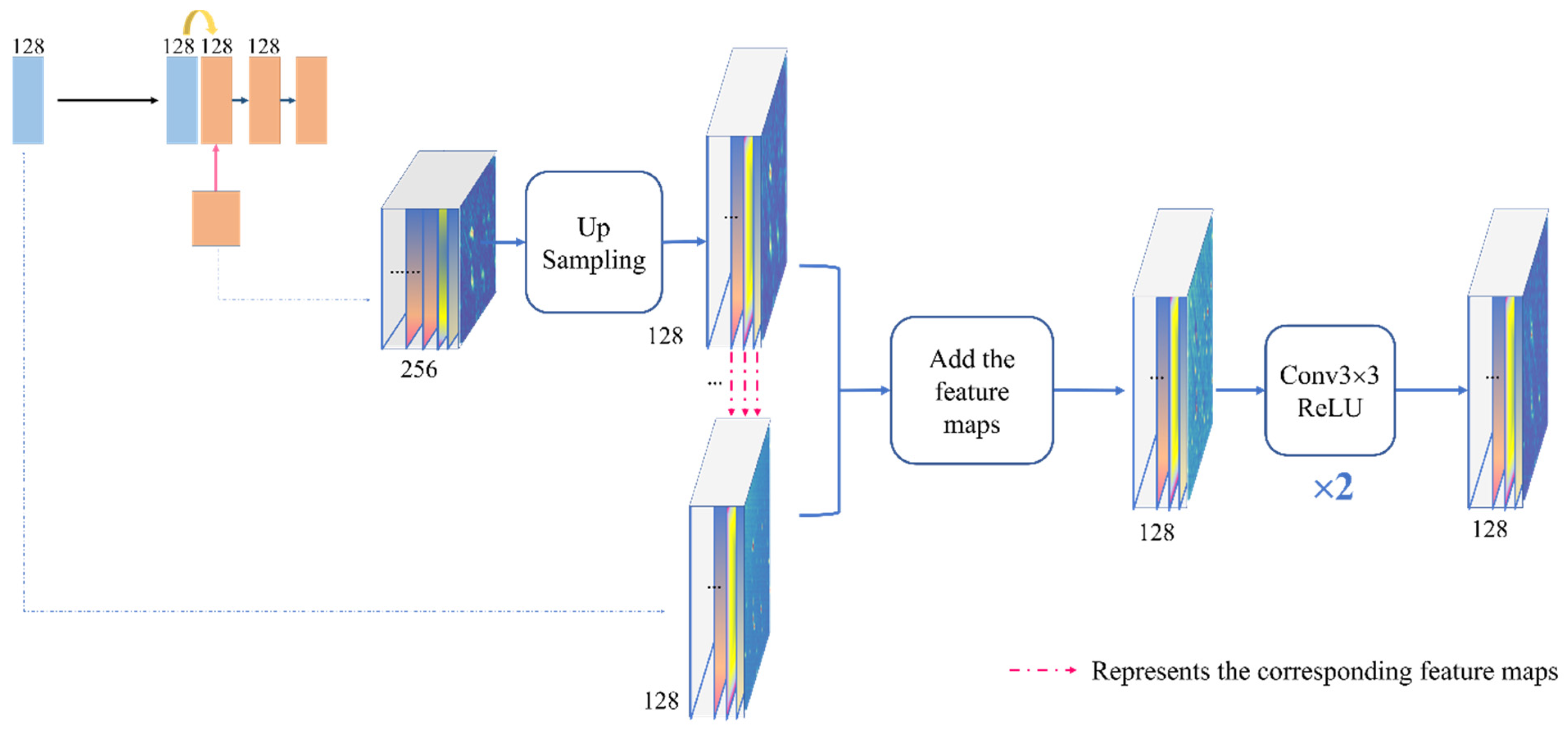
2.1.2. Foreground Retention Part
2.1.3. Strengths of BSC-Net
- The selected structure cleverly combines the functions of background weakening and foreground preservation of two parts in one network, which can compensate for blurring and distortion of the foreground caused by the background suppression part. Unlike our approach, existing algorithms often only concentrate on one of the two functions.
- Compared with the majority of convolutional networks, BSC-Net significantly reduces the number of convolutional layers. Except for the final output layer, each of the other convolutional layers only has two layers. On the one hand, too many convolution operations will increase the amount of computations, thus affecting the processing efficiency of the network. On the other hand, the receptive field reached 68 due to the down-sampling and convolution processing in the background suppression part, which is sufficient to handle the stars and targets in the range of 3 × 3–20 × 20.
- BSC-Net does not require image preparation, size restriction and manual feature construction. After BSC-Net processing, a clean image with background suppression is output with the size and dimensions unchanged.
2.2. Blended Loss Function of Smooth_L1&SSIM
2.3. Dataset Preparation of Real Images
3. Results
3.1. Experimental Environment
3.2. Evaluation Criteria of Background Supprssion Effectiveness
3.2.1. SNR of Targets
- 1.
- First, the evaluation range of single target is determined, and the pixels in that range are called I. A threshold segmentation of I will be done.where If is the foreground mask obtained by threshold segmentation, and the threshold is typically determined by the mean and variance.
- 2.
- If is dilated to remove the effect of the transition region, which contains uncleared stray light around the target.B is set to be a structure element of size 5. The area after the dilation operation is called If’.
- 3.
- The mask of the background is determined by inverting If’, which is called Ib.
- 4.
- If and Ib are matched with I, respectively, to obtain the foreground region IB and background region IF.
- 5.
- Calculating SNR.where , represent the mean of the foreground and background, respectively, and is the variance of the background.
3.2.2. SSIM and PSNR
3.3. Verification Experiment of Network Function
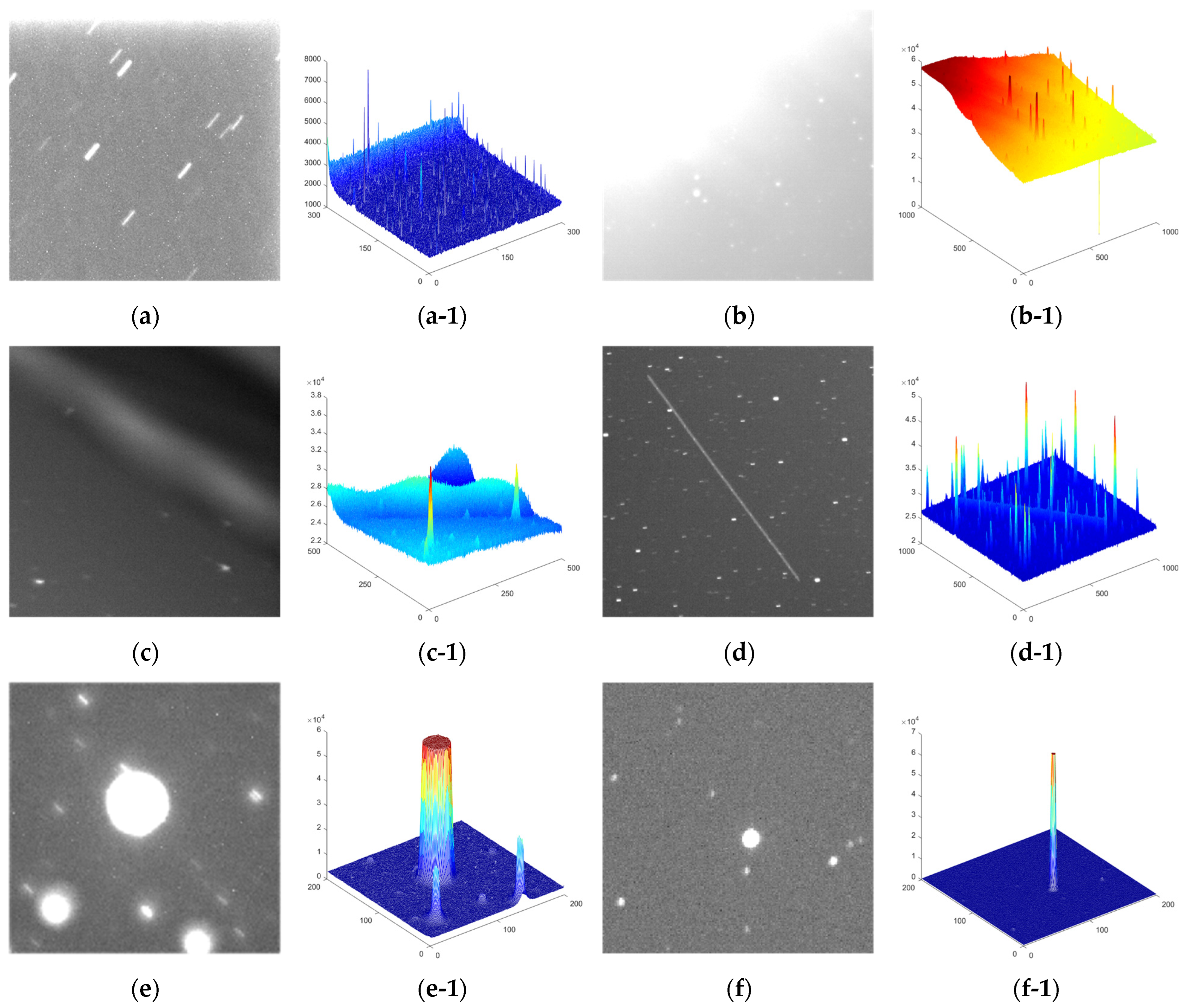
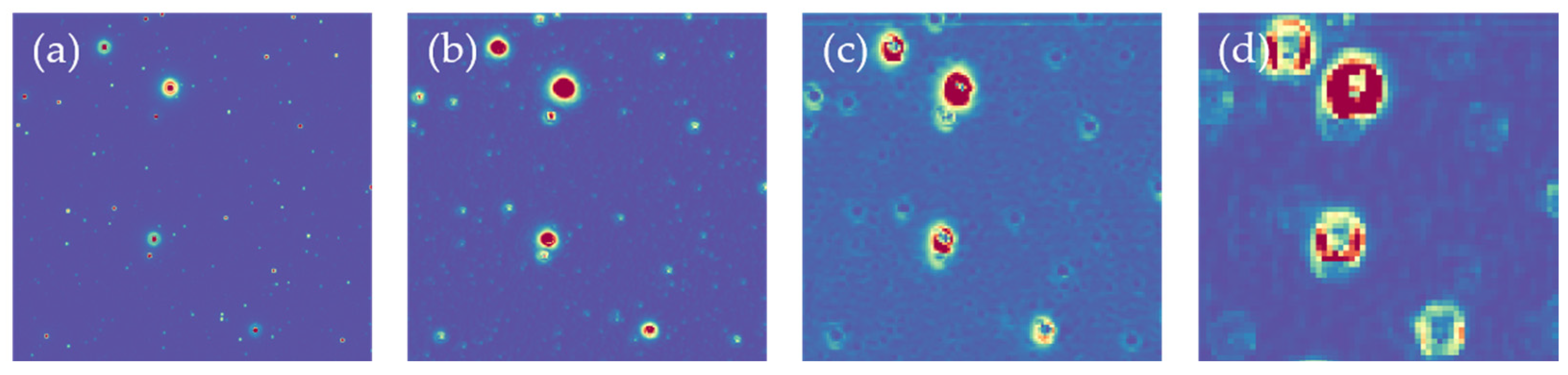
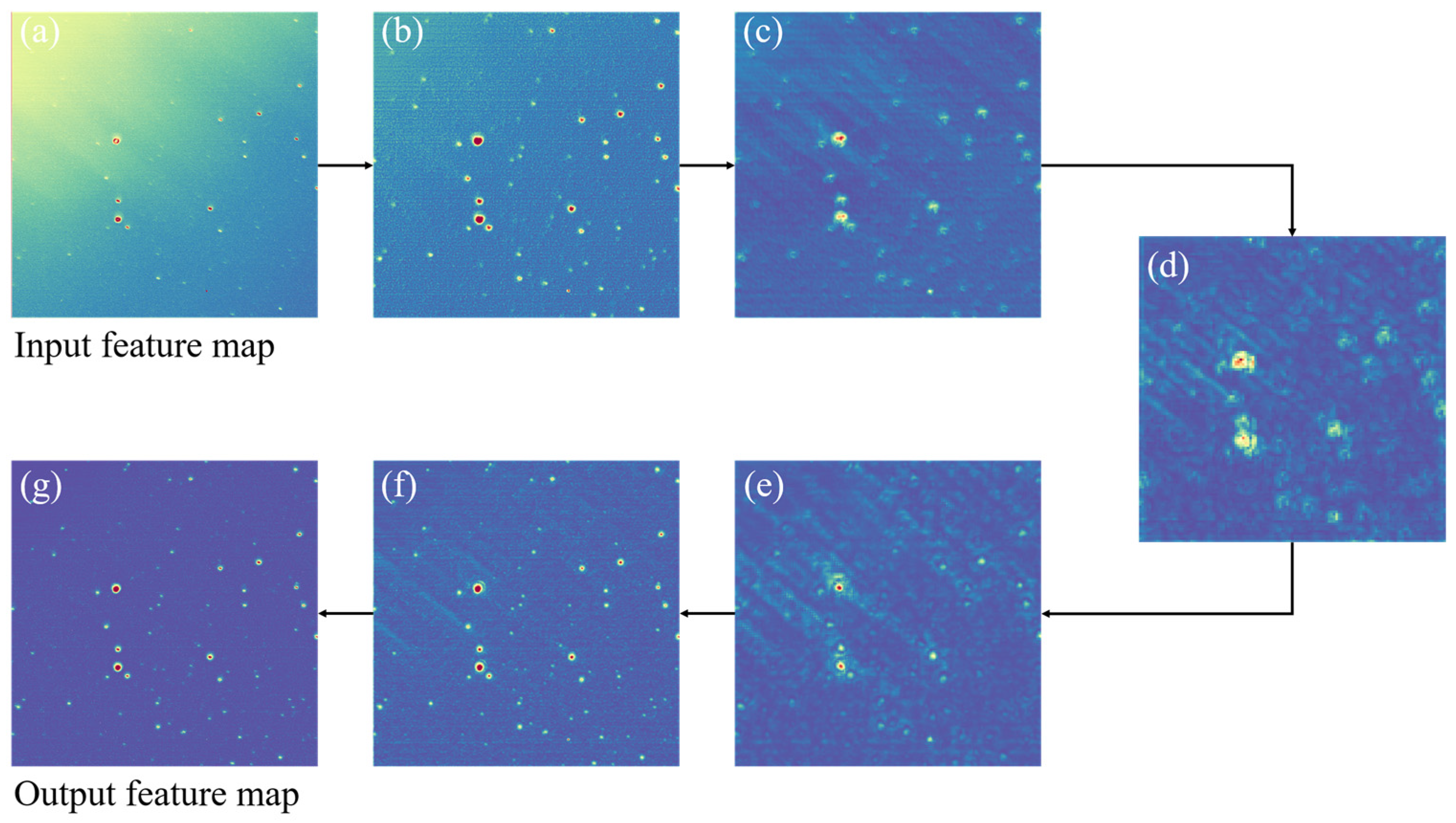
- The background suppression part of BSC-Net can achieve the expected effect. From Figure 9a–d, through down-sampling and convolution, the receptive field increases, the background in the image is gradually uniformized and the brightness is gradually weakened. Detail information in the foreground is reduced.
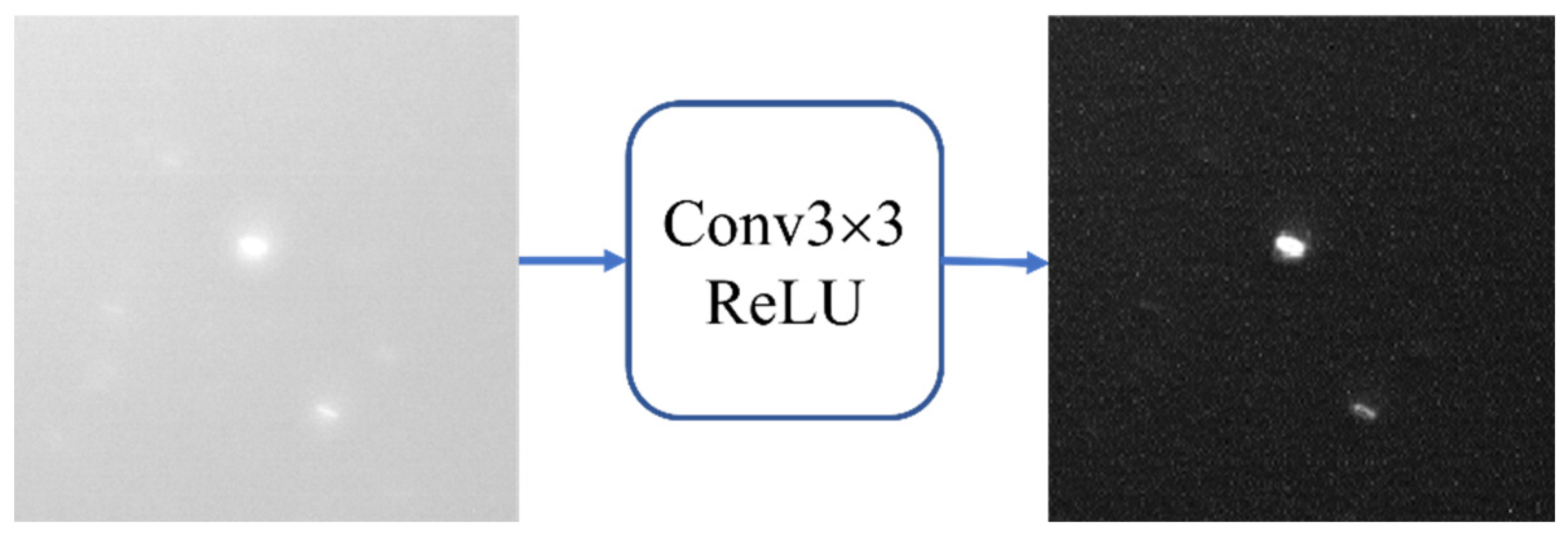
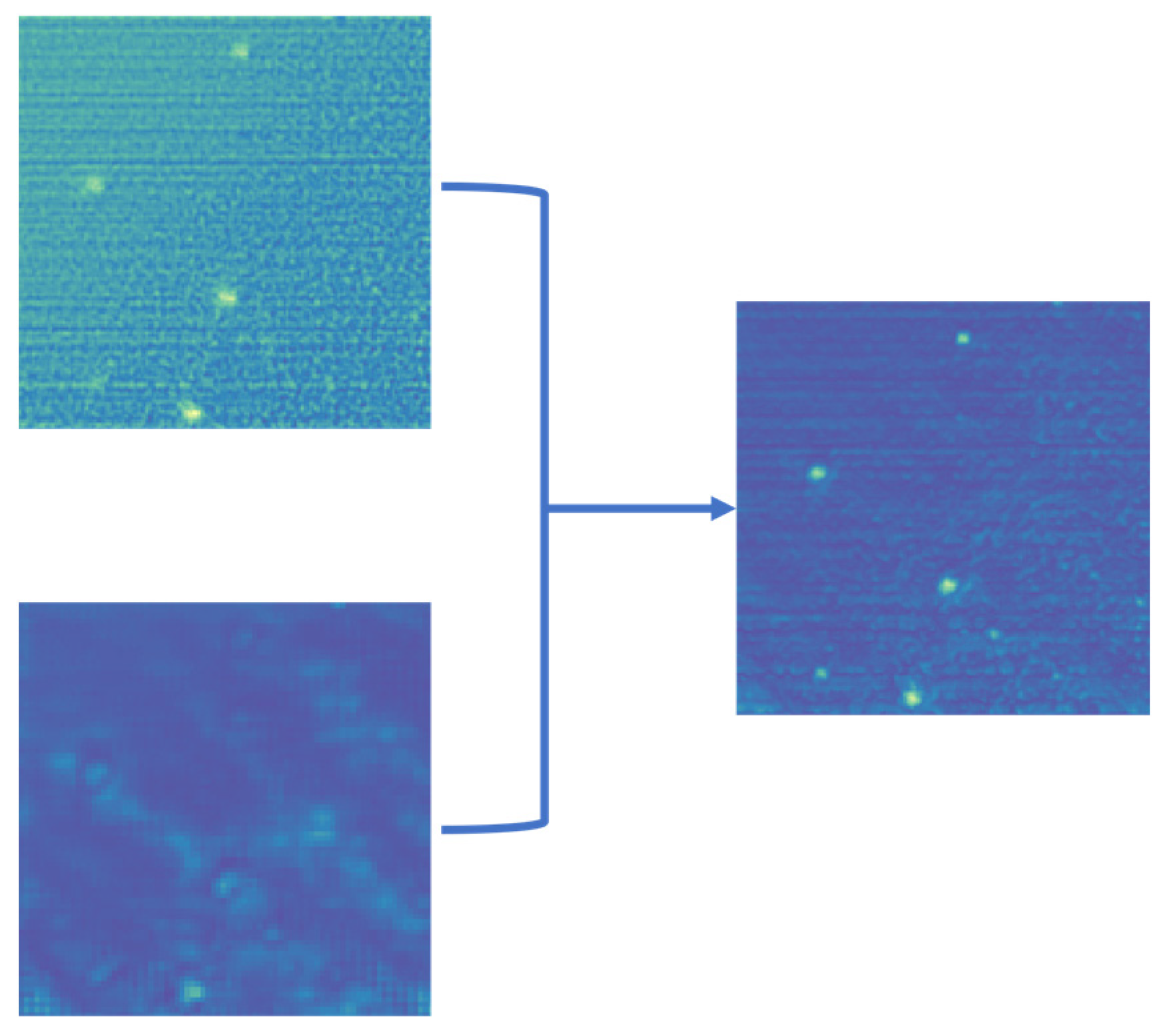
- The foreground retention part of BSC-Net can achieve the expected effect. From Figure 9e–g, through up-sampling and the skip connection, the detail information is completed, the foreground is preserved and the background is further suppressed by convolution. At the end, we get a clean output image.
3.4. Contrastive Experiment of Suppressing Stray Light
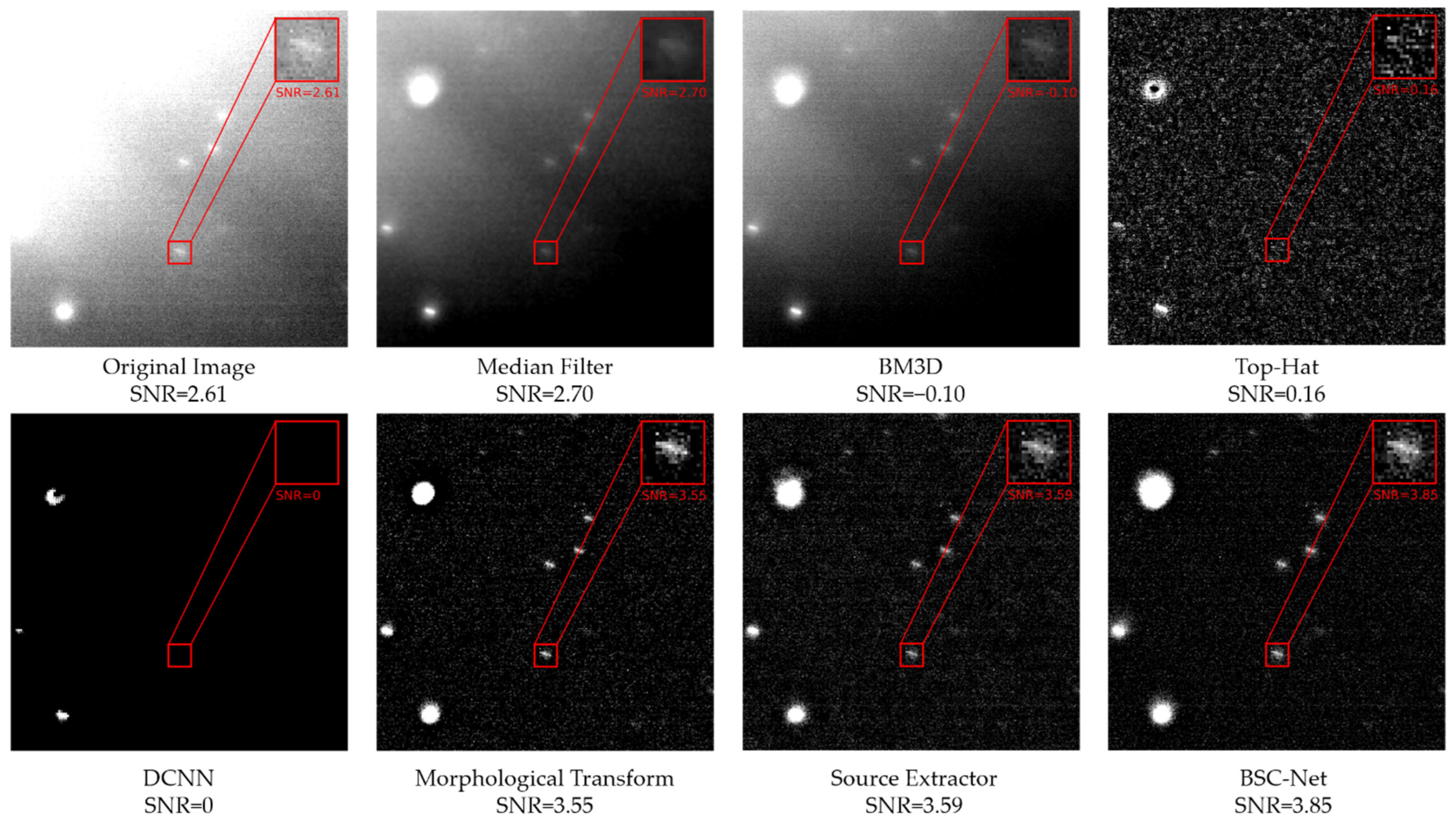
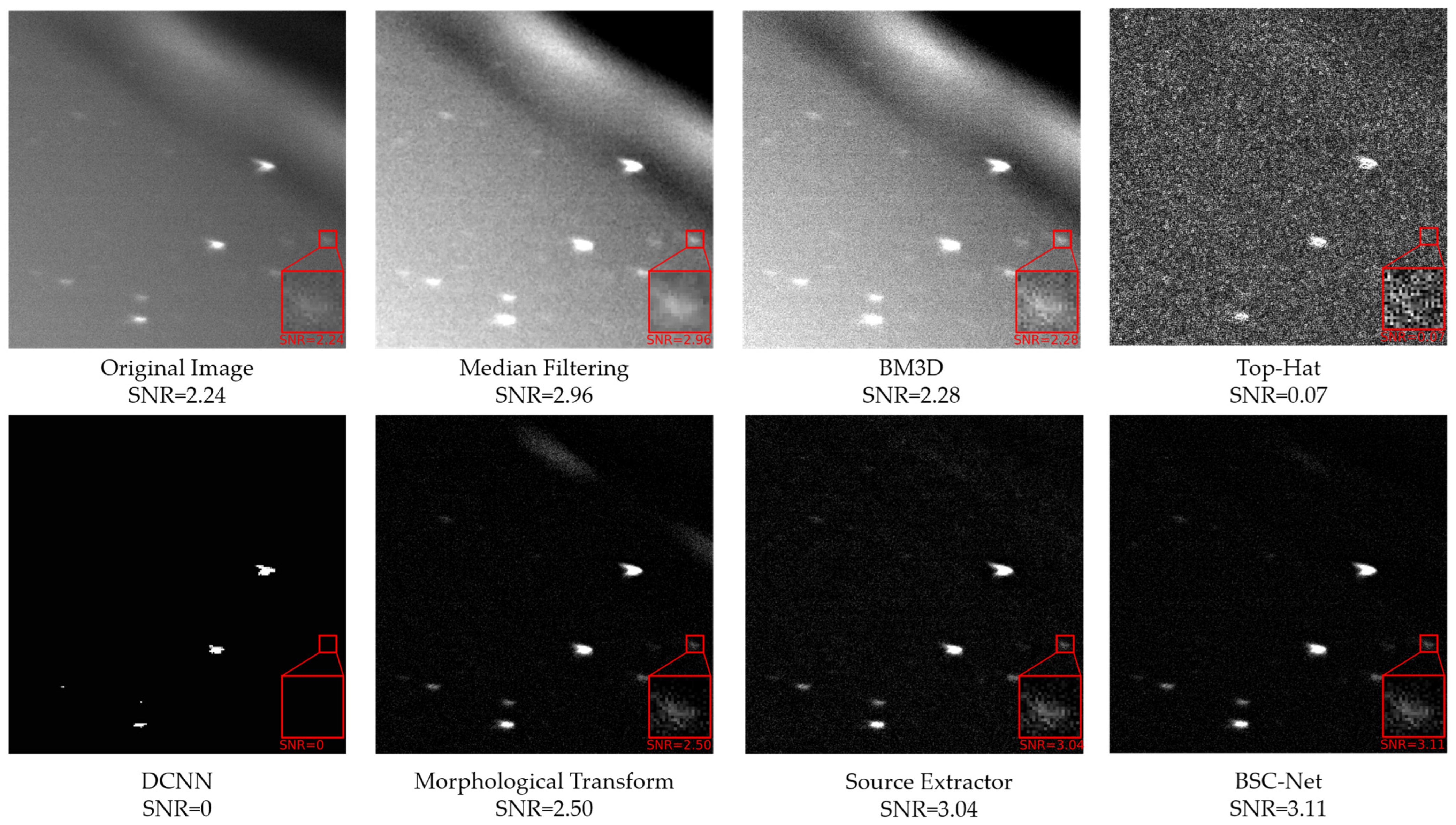
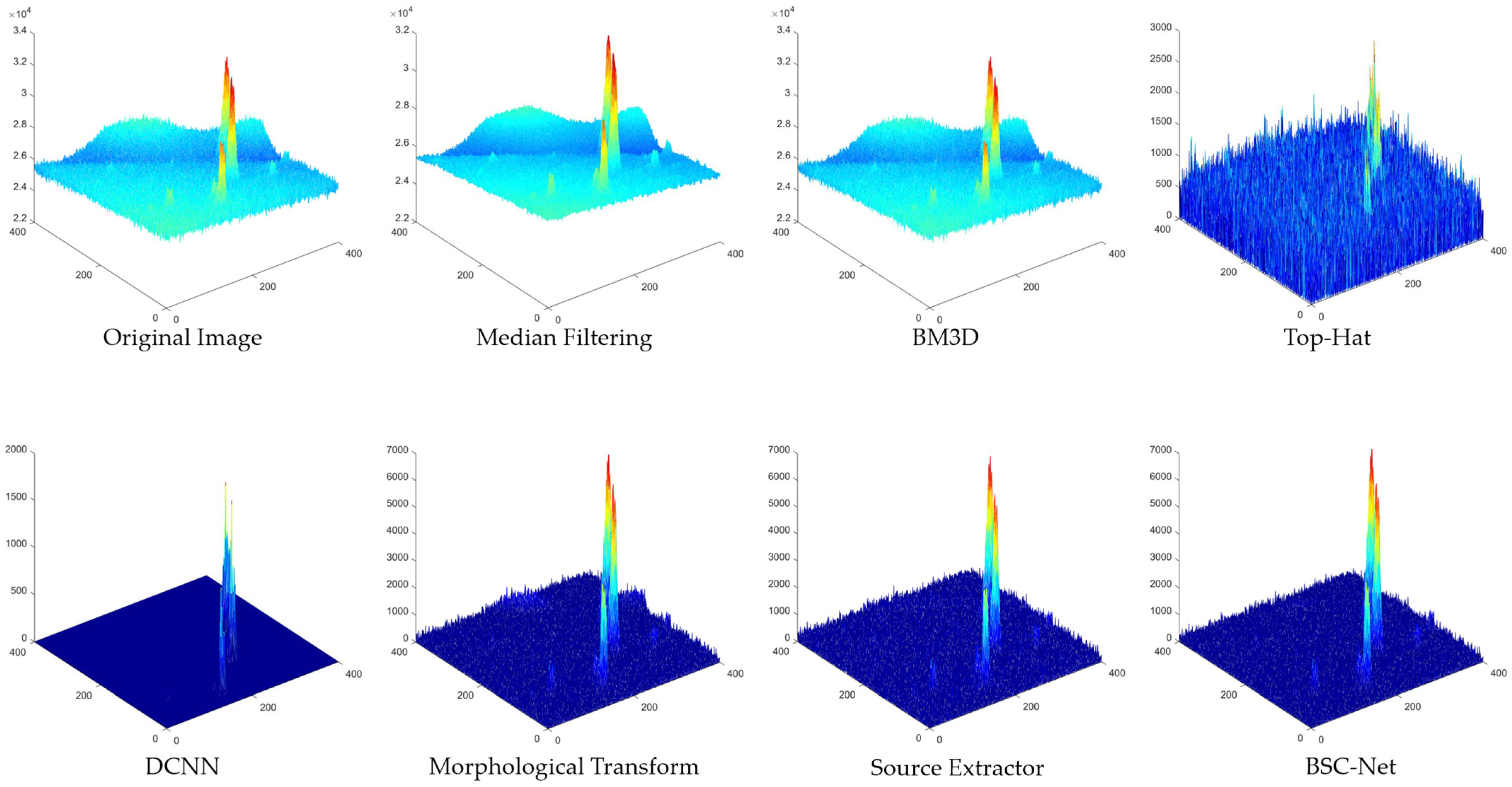
- Local highlight stray light: Figure 10 shows the results of local highlight stray light in different algorithms and the zoomed-in view of the dim target at the same location. It can be seen that BM3D and the median filter do not entirely eliminate background stray light. In BM3D, the average gray value of backgrounds is higher than that of the target, resulting in a negative SNR value. Top-Hat and DCNN over-eliminate the target and background, so the target information is almost lost, bringing the SNR value close to zero. The morphological approach and SExtractor both show positive results, but in terms of target retention, BSC-Net outperforms them.
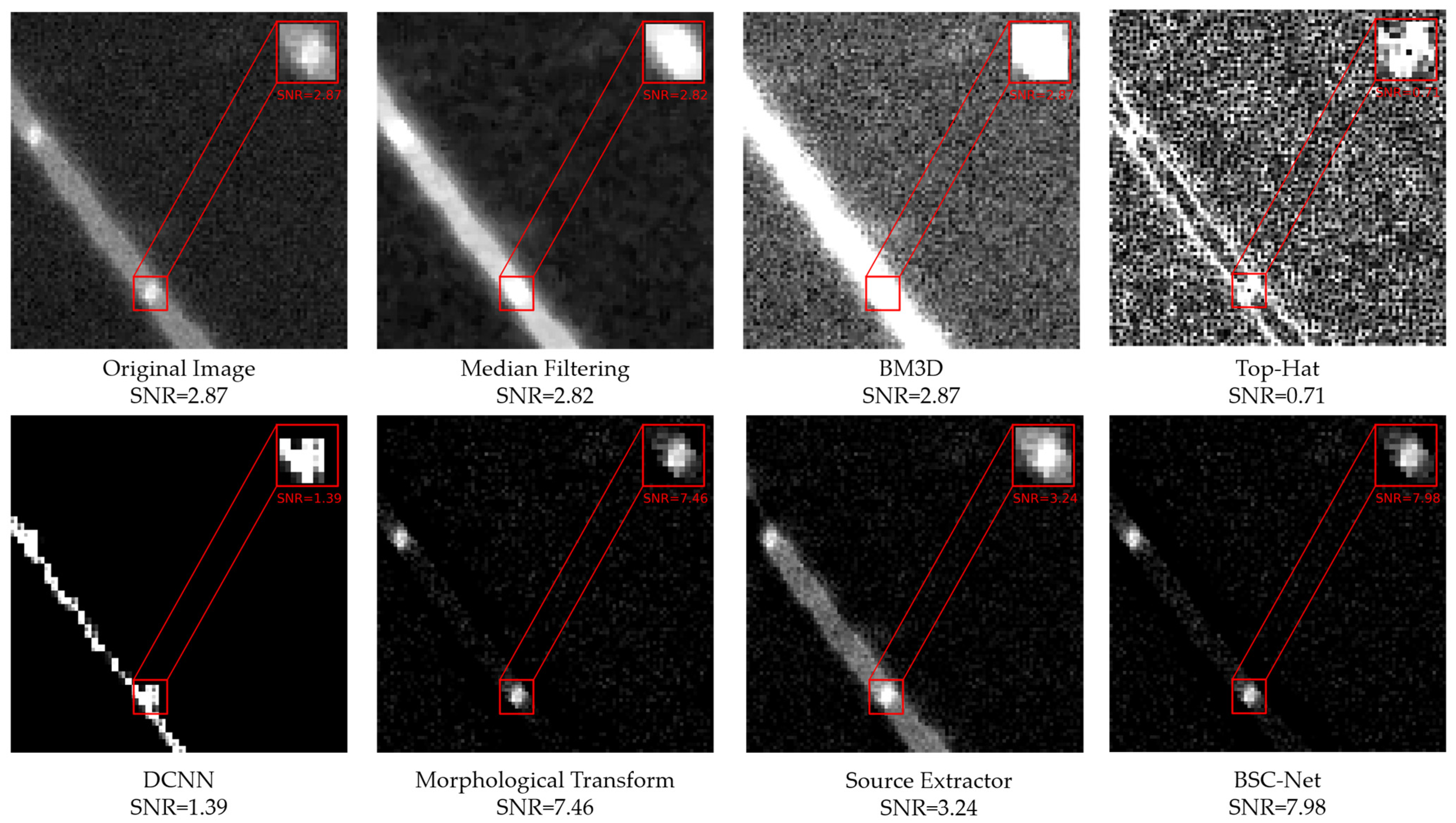
- Linear fringe interference: Figure 11 shows the results of linear fringe interference and the zoomed-in views. It can be found that the median filter and BM3D treat the target and the stray light as a whole while their gray values are similar, so that the contrast is reduced, and the SNR is lower than the original image. The target’s form is altered by Top-Hat and DCNN, while the high background variance causes the SNR to decrease. SExtractor suppresses most of the background, except for the fringe interference, but its effect is not significant in improving the target SNR. The stray light background is effectively suppressed by both the morphological method and BSC-Net, but BSC-Net has more advantages in terms of the SNR value.
- 3.
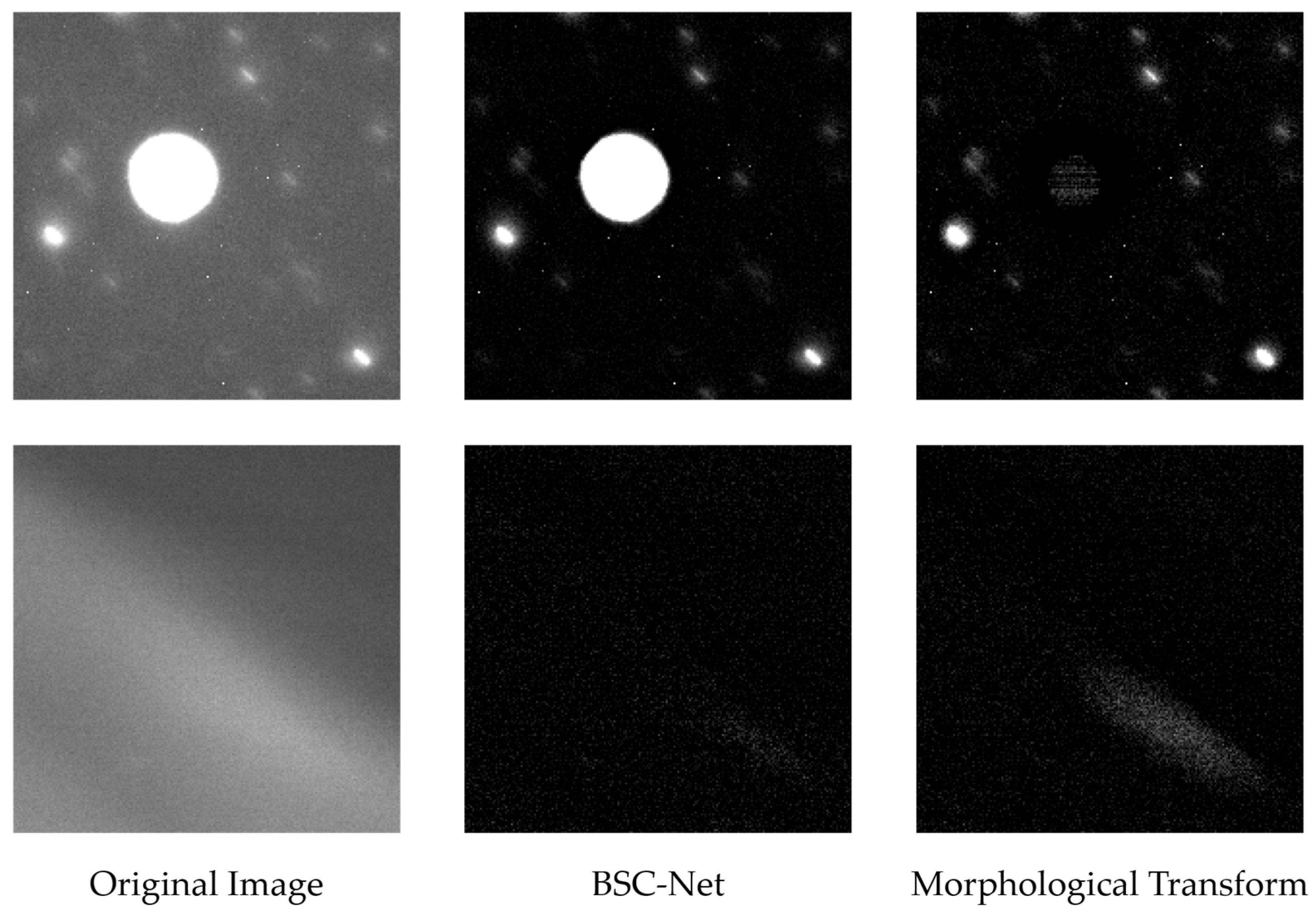
- Clouds occlusion stray light: Figure 12 shows the results of clouds covering stray light and the zoomed-in views. In the figure, the median filter and BM3D both improve the SNR and make the distinction between foreground and background more evident, but the suppression effect of the two on cloud occlusion is weak. The Top-Hat algorithm is less robust for this kind of image, as the target information is lost, and the SNR is near to zero. While DCNN reduces the stray light, it also eliminates foreground clutter. The morphological method, SExtractor and BSC-Net all suppress the stray light to a certain extent, but BSC-Net achieves better target preservation and higher SNR improvement.
3.5. Quantitative Evaluation Results for Different Datasets
4. Discussion
4.1. Analysis of the Network Structure
4.2. Analysis of Results
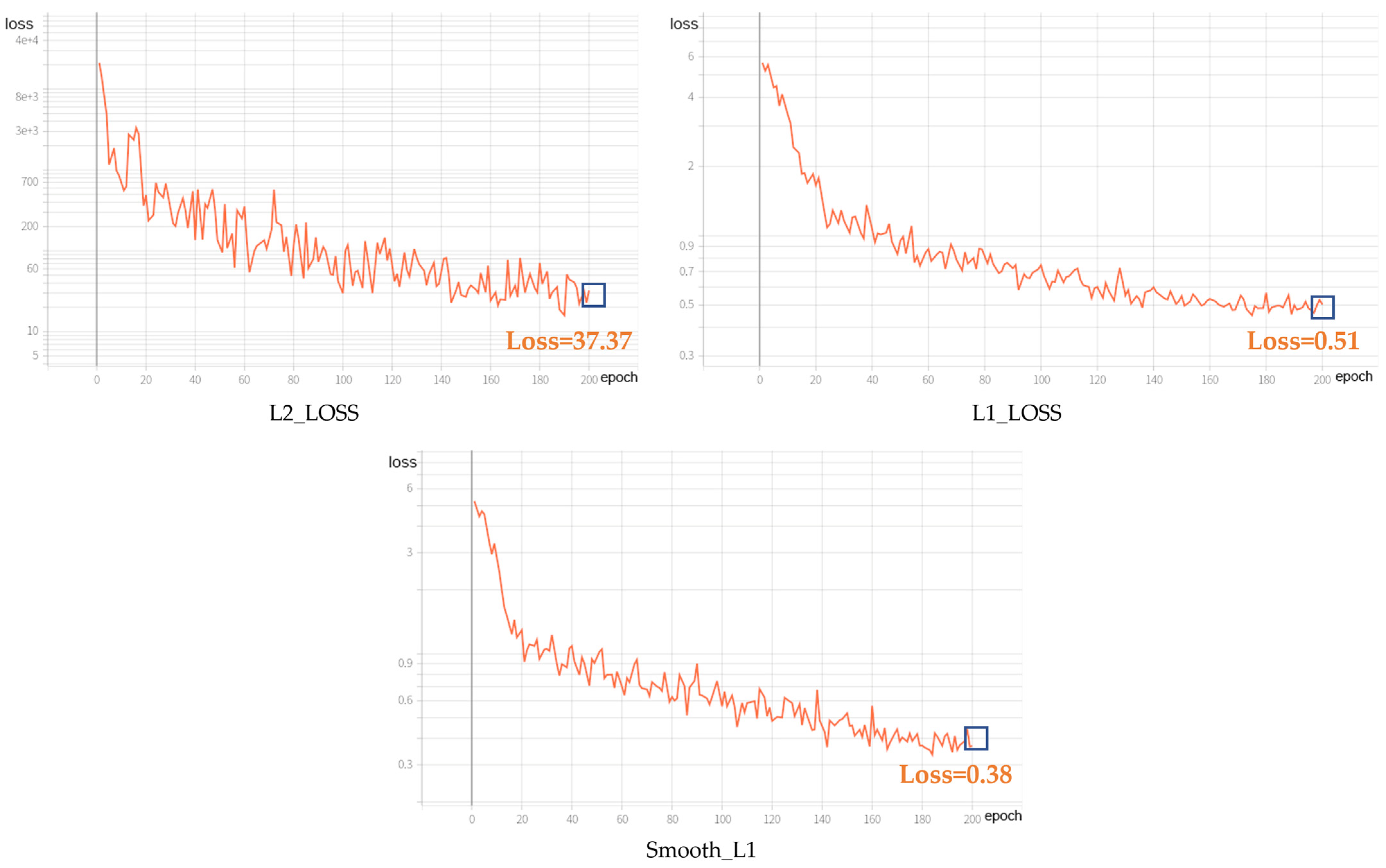
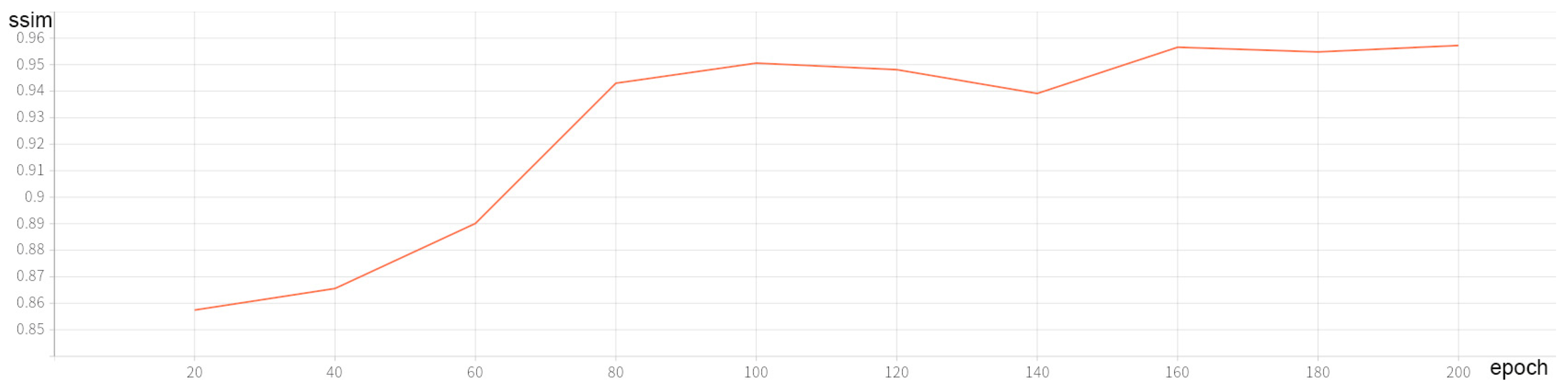
4.3. Analysis of Loss Function
5. Conclusions
Author Contributions
Funding
Data Availability Statement
Acknowledgments
Conflicts of Interest
Appendix A
References
- Schildknecht, T. Optical Surveys for Space Debris. Astron. Astrophys. Rev. 2007, 14, 41–111. [Google Scholar] [CrossRef]
- Li, Z.; Wang, Y.; Zheng, W. Space-Based Optical Observations on Space Debris via Multipoint of View. Int. J. Aerosp. Eng. 2020, 2020, 8328405. [Google Scholar] [CrossRef]
- Jiang, W.L.; Li, G.L.; Luo, W.B. Application of Improved Median Filtering Algorithm to Image Denoising. Adv. Mater. Res. 2014, 998–999, 838–841. [Google Scholar]
- Ruia, Y.; Yan-ninga, Z.; Jin-qiub, S.; Yong-penga, Z. Smear Removal Algorithm of CCD Imaging Sensors Based on Wavelet Transform in Star-sky Image. Acta Photonica Sin. 2011, 40, 413–418. [Google Scholar] [CrossRef]
- Dabov, K.; Foi, A.; Katkovnik, V.; Egiazarian, K. Image Denoising by Sparse 3-D Transform-Domain Collaborative Filtering. IEEE Trans. Image Process. 2007, 16, 2080–2095. [Google Scholar] [CrossRef] [PubMed]
- Yair, W.; Erick, F. Contour Extraction of Compressed JPEG Images. J. Graph. Tools 2001, 6, 37–43. [Google Scholar] [CrossRef]
- Bertin, E.; Arnouts, S. SExtractor: Software for source extraction. Astron. Astrophys. Suppl. Ser. 1996, 117, 393–404. [Google Scholar] [CrossRef]
- Wang, X.; Zhou, S. An Algorithm Based on Adjoining Domain Filter for Space Image Background and Noise Filtrating. Comput. Digit. Eng. 2012, 40, 98–99, 135. [Google Scholar]
- Yan, M.; Fei, W.U.; Wang, Z. Removal of SJ-9A Optical Imagery Stray Light Stripe Noise. Spacecr. Recovery Remote Sens. 2014, 35, 72–80. [Google Scholar]
- Chen, H.; Zhang, Y.; Zhu, X.; Wang, X.; Qi, W. Star map enhancement method based on background suppression. J. PLA Univ. Sci. Technol. Nat. Sci. Ed. 2015, 16, 7–11. [Google Scholar]
- Wang, W.; Wei, X.; Li, J.; Wang, G. Noise Suppression Algorithm of Short-wave Infrared Star Image for Daytime Star Sensor. Infrared Phys. Technol. 2017, 85, 382–394. [Google Scholar] [CrossRef]
- Zhang, X.; Lin, B.; Yang, X.; Wang, K.; Zhang, X. Stray light noise removal method of star maps based on intensity prior. J. Appl. Opt. 2021, 42, 454–461. [Google Scholar]
- Zou, Y.; Zhao, J.; Wu, Y.; Wang, B. Segmenting Star Images with Complex Backgrounds Based on Correlation between Objects and 1D Gaussian Morphology. Appl. Sci. 2021, 11, 3763. [Google Scholar] [CrossRef]
- Wang, X.W.; Liu, J. A noise suppression method for 16-bit starry background image. Electron. Opt. Control. 2022, 29, 66–69. [Google Scholar]
- Tian, C.; Fei, L.; Zheng, W.; Xu, Y.; Zuo, W.; Lin, C.W. Deep learning on image denoising: An overview. Neural Netw. 2020, 131, 251–275. [Google Scholar] [CrossRef]
- Guo, S.; Yan, Z.; Zhang, K.; Zuo, W.; Zhang, L. Toward Convolutional Blind Denoising of Real Photographs. In Proceedings of the 2019 IEEE/CVF Conference on Computer Vision and Pattern Recognition (CVPR), Long Beach, CA, USA, 15–20 June 2019; pp. 1712–1722. [Google Scholar] [CrossRef]
- Liu, G.; Yang, N.; Guo, L.; Guo, S.; Chen, Z. A One-Stage Approach for Surface Anomaly Detection with Background Suppression Strategies. Sensors 2020, 20, 1829. [Google Scholar] [CrossRef]
- Francesco, D.; Fabio, S.; Fabrizio, P.; Fortunatoc, V.; Abbattistac, C.; Amorusoc, L. Efficient and automatic image reduction framework for space debris detection based on GPU technology. Acta Astronaut. 2018, 145, 332–341. [Google Scholar]
- Sun, J.; Cao, W.; Xu, Z.; Ponce, J. Learning a convolutional neural network for non-uniform motion blur removal. In Proceedings of the 2015 IEEE Conference on Computer Vision and Pattern Recognition (CVPR), Boston, MA, USA, 7–12 June 2015; pp. 769–777. [Google Scholar] [CrossRef]
- Nah, S.; Kim, T.H.; Lee, K.M. Deep Multi-scale Convolutional Neural Network for Dynamic Scene Deblurring. In Proceedings of the 2017 IEEE Conference on Computer Vision and Pattern Recognition (CVPR), Honolulu, HI, USA, 21–26 July 2017; pp. 257–265. [Google Scholar] [CrossRef]
- Liang-Kui, L.; Shao-You, W.; Zhong-Xing, T. Point target detection in infrared over-sampling scanning images using deep convolutional neural networks. J. Infrared Millim. Waves 2018, 37, 219. [Google Scholar]
- Zhang, K.; Gao, X.; Tao, D.; Li, X. Single Image Super-Resolution With Non-Local Means and Steering Kernel Regression. IEEE Trans. Image Process. 2012, 21, 4544–4556. [Google Scholar] [CrossRef]
- Mao, X.; Shen, C.; Yang, Y. Image restoration using very deep convolutional encoder-decoder networks with symmetric skip connections. In Proceedings of the 30th International Conference on Neural Information Processing Systems (NIPS’16), Barcelona, Spain, 5–10 December 2016; Curran Associates Inc.: Red Hook, NY, USA, 2016; pp. 2810–2818. [Google Scholar]
- Zhang, K.; Zuo, W.; Zhang, L. FFDNet: Toward a Fast and Flexible Solution for CNN-Based Image Denoising. IEEE Trans. Image Process. 2018, 27, 4608–4622. [Google Scholar] [CrossRef]
- Zhang, K.; Zuo, W.; Chen, Y.; Meng, D.; Zhang, L. Beyond a Gaussian Denoiser: Residual Learning of Deep CNN for Image Denoising. IEEE Trans. Image Process. 2017, 26, 3142–3155. [Google Scholar] [CrossRef] [PubMed]
- Chen, J.; Chen, J.; Chao, H.; Yang, M. Image Blind Denoising with Generative Adversarial Network Based Noise Modeling. In Proceedings of the 2018 IEEE/CVF Conference on Computer Vision and Pattern Recognition, Salt Lake City, UT, USA, 18–23 June 2018; pp. 3155–3164. [Google Scholar] [CrossRef]
- Liu, Y.; Zhao, C.; Xu, Q. Neural Network-Based Noise Suppression Algorithm for Star Images Captured During Daylight Hours. Acta Opt. Sin. 2019, 39, 0610003. [Google Scholar]
- Xue, D.; Sun, J.; Hu, Y.; Zheng, Y.; Zhu, Y.; Zhang, Y. Dim small target detection based on convolutinal neural network in star image. Multimed Tools Appl. 2020, 79, 4681–4698. [Google Scholar] [CrossRef]
- Xie, M.; Zhang, Z.; Zheng, W.; Li, Y.; Cao, K. Multi-Frame Star Image Denoising Algorithm Based on Deep Reinforcement Learning and Mixed Poisson–Gaussian Likelihood. Sensors 2020, 20, 5983. [Google Scholar] [CrossRef]
- Zhang, Z.; Zheng, W.; Ma, Z.; Yin, L.; Xie, M.; Wu, Y. Infrared Star Image Denoising Using Regions with Deep Reinforcement Learning. Infrared Phys. Technol. 2021, 117, 103819. [Google Scholar] [CrossRef]
- Xi, J.; Wen, D.; Ersoy, O.K.; Yi, H.; Yao, D.; Song, Z.; Xi, S. Space debris detection in optical image sequences. Appl. Opt. 2016, 55, 7929–7940. [Google Scholar] [CrossRef]
- Zhang, C.; Zhang, H.; Yuan, B.; Hu, L. Estimation of Star-sky Image Background and Its Application on HDR Image Enhancement. J. Telem. Track. Command. 2013, 4, 22–27. [Google Scholar]
- Zhang, H.; Hao, Y.J. Simulation for View Field of Star Sensor Based on STK. Comput. Simul. 2011, 7, 83–86, 94. [Google Scholar]
- Wang, Y.; Niu, Z.; Wang, D.; Huang, J.; Li, P.; Sun, Q. Simulation Algorithm for Space-Based Optical Observation Images Considering Influence of Stray Light. Laser Optoelectron. Prog. 2022, 59, 0229001. [Google Scholar]
- Wang, Z.; Simoncelli, E.P.; Bovik, A.C. Multiscale structural similarity for image quality assessment. In Proceedings of the Thrity-seventh Asilomar Conference on Signals, Systems Computers, Pacific Grove, CA, USA, 9–12 November 2003; Volume 2003, pp. 1398–1402. [Google Scholar]
- Ronneberger, O.; Fischer, P.; Brox, T. U-Net: Convolutional Networks for Biomedical Image Segmentation. In Medical Image Computing and Computer-Assisted Intervention–MICCAI 2015; Navab, N., Hornegger, J., Wells, W., Frangi, A., Eds.; Lecture Notes in Computer Science; Springer: Cham, Switzerland, 2015; Volume 9351. [Google Scholar] [CrossRef]
- Girshick, R. Fast R-CNN. In Proceedings of the 2015 IEEE International Conference on Computer Vision (ICCV), Santiago, Chile, 7–13 December 2015; pp. 1440–1448. [Google Scholar] [CrossRef]
- Naser, M.Z.; Alavi, A.H. Error Metrics and Performance Fitness Indicators for Artificial Intelligence and Machine Learning in Engineering and Sciences. Archit. Struct. Constr. 2021. [Google Scholar] [CrossRef]
- Botchkarev, A. A New Typology Design of Performance Metrics to Measure Errors in Machine Learning Regression Algorithms. Interdiscip. J. Inf. Knowl. Manag. 2019, 14, 45–79. [Google Scholar] [CrossRef]
- Bai, X.; Zhou, F.; Xue, B. Image enhancement using multi scale image features extracted by top-hat transform. Opt. Laser Technol. 2012, 44, 328–336. [Google Scholar] [CrossRef]
- Huang, J.; Wei, A.; Lin, Z.; Zhang, G. Multilevel filter background suppression algorithm based on morphology. Aerosp. Electron. Warf. 2015, 31, 55–58. [Google Scholar] [CrossRef]
- Tao, J.; Cao, Y.; Zhuang, L.; Zhang, Z.; Ding, M. Deep Convolutional Neural Network Based Small Space Debris Saliency Detection. In Proceedings of the 2019 25th International Conference on Automation and Computing (ICAC), Lancaster, UK, 5–7 September 2019; pp. 1–6. [Google Scholar]
- Peng, J.; Liu, Q.; Sun, Y. Detection and Classification of Astronomical Targets with Deep Neural Networks in Wide Field Small Aperture Telescopes. Astron. J. 2020, 159, 212. [Google Scholar] [CrossRef]
- Lv, P.-Y.; Sun, S.-L.; Lin, C.-Q.; Liu, G.-R. Space moving target detection and tracking method in complex background. Infrared Phys. Technol. 2018, 91, 107–118. [Google Scholar] [CrossRef]
- Jung, K.; Lee, J.-I.; Kim, N.; Oh, S.; Seo, D.-W. Classification of Space Objects by Using Deep Learning with Micro-Doppler Signature Images. Sensors 2021, 21, 4365. [Google Scholar] [CrossRef]
- Liu, X.; Li, X.; Li, L.; Su, X.; Chen, F. Dim and Small Target Detection in Multi-Frame Sequence Using Bi-Conv-LSTM and 3D-Conv Structure. IEEE Access 2021, 9, 135845–135855. [Google Scholar] [CrossRef]
- Yang, X.; Nan, X.; Song, B. D2N4: A Discriminative Deep Nearest Neighbor Neural Network for Few-Shot Space Target Recognition. IEEE Trans. Geosci. Remote Sens. 2020, 58, 3667–3676. [Google Scholar] [CrossRef]
- Han, J.; Yang, X.; Xu, T.; Fu, Z.; Chang, L.; Yang, C.; Jin, G. An End-to-End Identification Algorithm for Smearing Star Image. Remote Sens. 2021, 13, 4541. [Google Scholar] [CrossRef]
- Du, J.; Lu, H.; Hu, M.; Zhang, L.; Shen, X. CNN-based infrared dim small target detection algorithm using target-oriented shallow-deep features and effective small anchor. IET Image Process. 2021, 15, 1–15. [Google Scholar] [CrossRef]
- Li, M.; Lin, Z.-P.; Fan, J.-P.; Sheng, W.-D.; Li, J.; An, W.; Li, X.-L. Point target detection based on deep spatial-temporal convolution neural network. J. Infrared Millim. Waves 2021, 40, 122. [Google Scholar]
- Xiang, Y.; Xi, J.; Cong, M.; Yang, Y.; Ren, C.; Han, L. Space debris detection with fast grid-based learning. In Proceedings of the 2020 IEEE 3rd International Conference of Safe Production and Informatization (IICSPI), Chongqing, China, 28–30 November 2020; pp. 205–209. [Google Scholar] [CrossRef]
- Leung, H.; Dubash, N.; Xie, N. Detection of small objects in clutter using a GA-RBF neural network. IEEE Trans. Aerosp. Electron. Syst. 2002, 38, 98–118. [Google Scholar] [CrossRef]


| Methods | Original | Median Filter | BM3D | Top-Hat | DCNN | Source Extractor | BSC-Net | |
|---|---|---|---|---|---|---|---|---|
| Dataset | ||||||||
| Data1 1 | 4.40 | 4.41 | 4.40 | 41.36 | 42.44 | 48.57 | 50.86 | |
| Data2 1 | 7.74 | 7.74 | 7.74 | 44.36 | 52.20 | 43.89 | 65.89 | |
| Data3 1 | 30.18 | 30.20 | 30.18 | 57.86 | 60.74 | 63.28 | 71.77 | |
| Data4 1 | 3.95 | 3.85 | 3.85 | 42.44 | 50.95 | 43.95 | 55.90 | |
| Data5 1 | 8.19 | 8.19 | 8.19 | 45.91 | 50.16 | 52.07 | 62.73 | |
| Data6 1 | 52.69 | 50.01 | 52.71 | 71.54 | 52.20 | 78.62 | 79.69 | |
| Methods | Original | Median Filter | BM3D | TOPHAT | DCNN | Source Extractor | BSC-Net | |
|---|---|---|---|---|---|---|---|---|
| Dataset | ||||||||
| Data1 1 | 0.0045 | 0.0034 | 0.0045 | 0.1420 | 0.0015 | 0.0490 | 0.7697 | |
| Data2 1 | 0.0024 | 0.0012 | 0.0025 | 0.1402 | 0.0108 | 0.0331 | 0.8830 | |
| Data3 1 | 0.0069 | 0.0008 | 0.0045 | 0.1783 | 0.0539 | 0.0958 | 0.8905 | |
| Data4 1 | 0.0013 | 0.0005 | 0.0017 | 0.1235 | 0.0011 | 0.0396 | 0.8874 | |
| Data5 1 | 0.0034 | 0.0013 | 0.0033 | 0.1734 | 0.0003 | 0.0343 | 0.9175 | |
| Data6 1 | 0.0378 | 0.0174 | 0.0190 | 0.2419 | 0.1511 | 0.2283 | 0.8794 | |
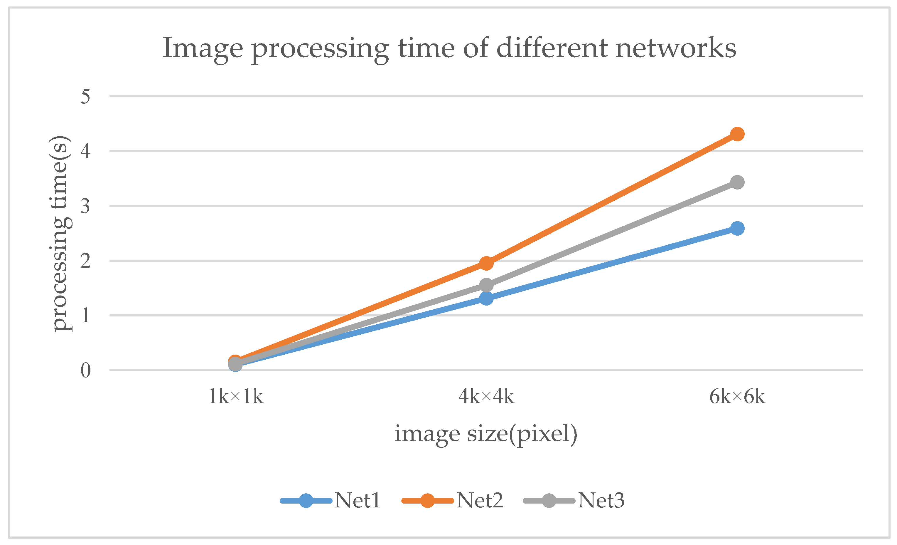
| Networks | SSIM | PSNR |
|---|---|---|
| Net1 | 0.933 | 64.90 |
| Net2 | 0.935 | 65.91 |
| Net3 | 0.935 | 67.50 |
Publisher’s Note: MDPI stays neutral with regard to jurisdictional claims in published maps and institutional affiliations. |
© 2022 by the authors. Licensee MDPI, Basel, Switzerland. This article is an open access article distributed under the terms and conditions of the Creative Commons Attribution (CC BY) license (https://creativecommons.org/licenses/by/4.0/).
Share and Cite
Li, Y.; Niu, Z.; Sun, Q.; Xiao, H.; Li, H. BSC-Net: Background Suppression Algorithm for Stray Lights in Star Images. Remote Sens. 2022, 14, 4852. https://doi.org/10.3390/rs14194852
Li Y, Niu Z, Sun Q, Xiao H, Li H. BSC-Net: Background Suppression Algorithm for Stray Lights in Star Images. Remote Sensing. 2022; 14(19):4852. https://doi.org/10.3390/rs14194852
Chicago/Turabian StyleLi, Yabo, Zhaodong Niu, Quan Sun, Huaitie Xiao, and Hui Li. 2022. "BSC-Net: Background Suppression Algorithm for Stray Lights in Star Images" Remote Sensing 14, no. 19: 4852. https://doi.org/10.3390/rs14194852
APA StyleLi, Y., Niu, Z., Sun, Q., Xiao, H., & Li, H. (2022). BSC-Net: Background Suppression Algorithm for Stray Lights in Star Images. Remote Sensing, 14(19), 4852. https://doi.org/10.3390/rs14194852