Article

A Methodology for National Scale Coastal Landcover Mapping in New Zealand

School of Environment, University of Auckland, 23 Symonds Street, Auckland 1142, New Zealand
*
Author to whom correspondence should be addressed.
Remote Sens. 2022, 14(19), 4827; https://doi.org/10.3390/rs14194827
Submission received: 29 July 2022 / Revised: 23 September 2022 / Accepted: 26 September 2022 / Published: 27 September 2022

Abstract

:
Satellite earth observation data has become fundamental in efforts to map coastal change at large geographic scales. Research has generally focussed on extracting the instantaneous waterline position from time-series of satellite images to interpret long-term trends. The use of this proxy can, however, be uncertain because the waterline is sensitive to marine conditions and beach gradient. In addition, the technique disregards potentially useful data stored in surrounding pixels. In this paper, we describe a pixel-based technique to analyse coastal change. A hybrid rule-based and machine learning methodology was developed using a combination of Sentinel multispectral and Synthetic Aperture Radar composite imagery. The approach was then used to provide the first national-scale pixel-based landcover classification for the open coast of New Zealand. Nine landcover types were identified including vegetation, rock, and sedimentary classes that are common on beaches (dark sand, light sand, and gravel). Accuracy was assessed at national scale (overall accuracy: 86%) and was greater than 90% when normalised for class area. Using a combination of optical and Synthetic Aperture Radar data improved overall accuracy by 14% and enhanced the separation of coastal sedimentary classes. Comparison against a previous classification approach of sandy coasts indicated improvements of 30% in accuracy. The outputs and code are freely available and open-source providing a new framework for per-pixel coastal landcover mapping for all regions where public earth observation data is available.

1. Introduction

Coastal regions are vulnerable to hazards, which can manifest at a range of temporal and spatial scales, caused by environmental and anthropogenic factors [1]. Human induced climate change is a leading driver of coastal change and adaptation at the coast is a key global issue [2]. Coastal monitoring plays an instrumental role in planning efforts to mitigate and adapt to future hazards such as erosion and flooding [2,3] and shoreline change investigations are considered an important part of such practises [4,5]. Remote sensing and land surveying techniques have been used to monitor change through repeat beach surveying or visual analysis of aerial photos [6,7,8]. In situ or airborne data, acquired from video imaging or Light detecting and ranging (LiDAR) sensors, can provide very-high spatial resolution data to monitor geomorphological features at beaches including the shoreline position [8] up to regional scales [9]. Acquisition of such data can be expensive, limiting temporal and spatial coverage [10]. Analyses of historic aerial photos can provide insights at greater geographic scale but are limited by temporal resolution and quality of available data [11].
Increased availability of earth observation satellite datasets provide global coverage at spatial/temporal resolutions highly suitable for shoreline mapping and at low costs compared to in situ surveying or aerial photography [8]. The development of cloud-computing platforms such as Google Earth Engine (GEE) [12] has further enhanced accessibility to these data archives, providing analysis ready imagery that is atmospherically corrected, orthorectified and easy to query in space and time. This has led to the development of new techniques to monitor change at the coast. To date, most efforts have focussed on extracting shoreline proxies/indicators from publicly available multispectral earth observation data archives such as Landsat or Sentinel with sub-pixel accuracy, deriving shoreline position with accuracies exceeding the native resolution of the sensor using interpolation techniques [13,14,15,16,17,18,19].

1.1. Shoreline Detection

Shoreline indicators can be defined as either a feature visible in imagery (e.g., most seaward vegetation line), the intersection of a tidal datum with a coastal or elevation profile (e.g., mean high water), or an indicator extracted through image processing techniques [4,20]. Most coastal change detection work with multispectral satellite imagery has focussed on extracting the instantaneous waterline (IW), where land and water are separated based on differences in spectral characteristics obtained from time-series of images to reveal a record of change to monitor short-term episodic events and long-term trends [20]. Information from such analyses is necessary for coastal management strategies, engineering and design of protection and, calibration/validation of coastal models [4].
Extracting the IW position from multispectral imagery can provide objective and repeatable approaches to assess coastal change at accuracies exceeding the spatial resolution of the satellite sensor, but the technique is not without uncertainties. Georeferencing errors of satellite imagery contribute positional uncertainty in derivation of the IW. The geometric accuracy of Landsat Tier 1 data, which is recommended for time-series analysis, is RMSE <12 m [21], which can be greater than the movement of the shoreline under investigation. Further uncertainty is caused by the environmental conditions of a given section of coast under investigation. The position of the IW is primarily driven by marine processes (waves/tides) and beach gradient. This can mean that for some coastal settings the spatiotemporal variation of the IW position can be up to hundreds of metres at near-instantaneous timescales where low gradient beaches are coupled with meso (2–4 m) or macro (>4 m) tidal conditions and large wave runup or swash [22,23]. Tidal influence has been corrected using compositing image techniques to limit short-term tidal variation [19,24]. More recently, combining composite techniques with tidal models has been implemented to remove images acquired at the highest and lowest observed tides to obtain composite images focused around a particular tidal datum [25]. Accounting for tidal influence is an important advancement that can remove some of the noise associated with IW position, but the presence of waves remains a complicating factor [23].
Assessing trends in IW shoreline position is considered an effective indicator of change, however not all drivers of change at the coast are associated with the movement of the IW shoreline position. Remote sensing methodologies that provide information beyond a single shoreline proxy should be investigated, because they are likely to contain valuable information on changes across the coastal zone, not just the land/water boundary.

1.2. Pixel-Based Techniques

Per-pixel classification techniques offer low cost methods for land cover/use mapping and change detection that can be implemented at large geographic scales [26]. A wide variety of methodologies have been applied to quantify and monitor a range of differing land cover types (e.g., forestry, mangroves, tidal zones and, surface water) from regional to global scales utilising freely available multispectral data from platforms such as Landsat or Sentinel [27,28,29,30]. Increased accessibility of cloud computing platforms that provide access to analysis ready earth observation data, such as GEE, mean that per-pixel techniques can be applied at increasingly larger scales without the requirement for local high-performance computers. Workflows can incorporate geospatial datasets from multiple sensor types such as multispectral and Synthetic Aperture Radar (SAR) efficiently without the requirement for complex pre-processing steps.
Despite the widespread use of pixel-based landcover classification in remote sensing, applying these methods for coastal research has remained limited to a small number of studies that have used pixel landcover classification to quantify sediment supply and vegetation cover to assess coastal change for barrier islands at regional scales [31,32]. A global approach [24] estimated that 31% of the world’s ice free coasts are sandy beaches using supervised image classification techniques, and [33] were able to estimate beach width by comparing vegetation areas with IW position. However, these approaches, among others, have continued to focus on the separation of land and water to detect the IW shoreline position [13,15,24,33], and potentially useful information stored in pixels beyond the land/water interface have been discarded. Further application of per-pixel classification techniques at the coast might enable monitoring of different coastal land cover types (e.g., sand and gravel sediments, rock, vegetation), with implications for coastal management. Successful per-pixel change detection requires a highly accurate land cover product [27]. This is a challenge at the coast over large geographic scales due to the complex physical characteristics and some classes that can be spectrally homogenous (e.g., sand and gravels) and difficult to separate using multispectral data alone.
The aim of this study is to develop and validate a hybrid rule-based and supervised machine learning classification workflow that identifies coastal specific land cover types for the New Zealand coastal zone from all Sentinel-1 (S1) and Sentinel-2 (S2) data available for 2019 to establish a specific coastal landcover classification. Annual composite images were derived and used in a per-pixel classification workflow that separates spectrally heterogeneous land cover types with a hierarchal set of rules. Remaining spectrally similar classes were classified using supervised machine learning that leverages both spectral and SAR data. This was trained with a manually derived national scale coastal specific training dataset. The final product was compared with the results obtained from a prior per-pixel approach [24]. The suitability of the methodology is evaluated and the temporal and spatial limitations are discussed in the context of coastal change monitoring at national to global scales.

2. Materials and Methods

2.1. New Zealand Coastal Setting

The New Zealand spans 13 degrees of latitude in the south-west Pacific with climates ranging from sub-tropical to sub-Antarctic (Figure 1). The coastline is diverse, and environments are dynamic and variable due to complex geology and a range of oceanographic and climatic settings [34].

2.1.1. Geological and Sedimentary Components

New Zealand’s land mass was formed from tectonic processes along the Pacific-Australia plate boundary occurring throughout the Quaternary [35]. These processes have shaped the New Zealand coast and continue to characterise coastal evolution [36]. Earthquakes have led to rapid uplift and subsidence in several regions, for example Hawkes Bay in 1931 and Kaikoura in 2016 [37,38]. In the North Island volcanism is a key source of sediment along the west coast [7]. Volcanism is less prevalent on the South Island but uplift in the Southern Alps provides large quantities of granular material, via fluvial transport, to both the east and west coasts [36].
The diversity in sediment sources delivered to New Zealand’s coast results in varied spatial distributions at local to regional scales, sometimes over small geographic extents (Figure 1). This is evident, for example, in the Auckland region where the sources of sediment on the west coast are characterised as dark sands which contain high concentrations of heavy minerals such as plagioclase, augite, and titanomagnetite [39] and the east coast which is predominantly comprised of light sands that are typically dominated by minerals such as quartz, feldspar and lithic/shell fragments [40,41].

2.1.2. Climatic Processes

New Zealand’s coastline is exposed to waves from all directions and the full progression of the tidal wave [36]. Hindcasts used to generate a wave climate of NZ indicate that the highest wave energy is found along the south and southwest coasts, and less wave energy reaches the eastern and northern coasts due to sheltering and decreased fetch [42,43,44]. Alburquerque et al. [42] found mean nearshore significant wave height ( H s ) in the southwest of the South Island was 3.4 m which decreased north-eastwards.
The east coast of both islands H s was lower (1.6–1.9 m) due to shelter from prevailing southwest waves. Due to the distribution of wave energy, different regimes have been described for the east and west coasts of both islands [45]. Marine processes on the west coasts are controlled by high-energy long period swells that lead to wave-dominated settings [7,46]. Along east-facing coasts, it appears that climatic phases such as La Niña, associated with pacific decadal oscillation, influence coastal systems due to the impact of episodic storm events under these conditions [11,36].

2.2. Image Composite Development

The variability of the geological, sedimentary and climatic components of the coastal system in New Zealand means that coastal morphology is complex. Any classification workflow must be representative of multiple physical characteristics of the environmental settings under investigation. Local to regional variations in sediment composition, for instance, can vary across small spatial scales (e.g., two beaches next to each other).
GEE was used to process imagery from S1 and S2 for 2019 and generate SAR and multispectral composite images (Figure 2). The year 2019 was selected as this was the most recent year where both satellite imagery and ancillary data used to validate and train the classification was available at the national scale. Composites were generated from aggregations of pixel values from multiple images in a given time period. A benefit of this technique is that errors associated with cloud cover and marine processes (waves and tides) driving short-term and episodic variation are minimised [19,28]. Compositing images through time can strip temporal information, but for the purpose of establishing a baseline to assess long-term change, this is a simple technique for handling noise associated with short-term processes. S1 and S2 data are available in GEE in analysis-ready formats. Both Level-1C top-of-atmosphere and 2A surface reflectance S2 datasets are available where atmospheric correction is performed using Sen2Cor [47].
S1 Ground Range Detected (GRD) data is available where thermal noise removal, radiometric calibration, and terrain correction pre-processing steps have been applied and values are reported as sigma nought ( σ 0 ) backscatter coefficient [48]. A 3 km coastal zone was established for the entire New Zealand coastline using a 1.5 km buffer around the mean high water mark from the New Zealand Topo50 1:50,000 topographic dataset [49]. All scenes acquired from both sensors in 2019 that intersected with the coastal zone were used. Table 1 provides a full summary of the composite image bands passed to the classification workflow.

2.2.1. Multispectral Composite

A series of statistical aggregations of all selected pixel values were generated to create a multiband composite image. A total of 3929 Top-of-atmosphere (TOA) and 2354 surface reflectance (SR) images were used to derive annual composite images for 2019. SR images ensure that multi-temporal data is comparable by correcting for atmospheric conditions at the time each image was acquired [50]. However, issues exist with SR images in coastal regions where the area of land in a scene is small relative to adjacent water that have been found to effect the calculation of water based indices [21,51,52]. To address this, several remote sensing methodologies have utilised S2 TOA image collections with water-based indices where imagery is focussed around the coast [13,19,28,53]. The number of SR images available in GEE is also lower than TOA collection as not all images have been processed to SR. Hagenaars et al. [19] found that the more data used to generate temporal composites improved the accuracy of annual mean shoreline positions. As water indices were more sensitive to short-term temporal variation associated with marine processes, the TOA collection was used to generate water indices to maximise the number of images available to ensure minimal short-term noise. SR collections were used to generate composite multispectral bands (visible to shortwave infrared), and vegetation indices (Figure 3).
S2 scenes where cloud cover exceeded 20% were omitted and cloud masking was performed scene-by-scene using the cloud probability mask generated from the Sen2Cor algorithm. The spatial resolution of the visible and near-infrared (NIR) bands were resampled using nearest neighbour interpolation to 20 m to match the shortwave-infrared bands. Normalised difference vegetation index (NDVI) [54] was calculated using the following equation:
N D V I = N I R R N I R + R
where N I R is the near-infrared band and R is the red band. This was done for all SR images to derive the NDVI mean between the range of the 10th and 90th percentile, referred to as the interval mean. TOA images were used to calculate NDWI [55], MNDWI [56], and automated water extraction index (AWEI) [57] using the following expressions:
N D W I = G S W I R 1 G + S W I R 1
M N D W I = G N I R G + N I R
A W E I n s h = 4 ( G S W I R 1 ) ( 0.25 N I R + 2.75 S W I R 2 )
where G is the green band, S W I R 1 and S W I R 2 are the first and second shortwave-infrared bands, respectively. A W E I n s h was used as the impact of shadow was considered minimal as the focus was open coastal areas [57]. Water indices were also calculated for all images in the TOA collection and composite bands for the minimum, maximum, standard deviation and percentile (10, 25, 50, 75, 90) pixel values were generated. SR images were used to derive composite bands for the 15th percentile value for each S2 multispectral band, this was an extra precaution to remove cloud and shadow pixels missed by the cloud probability mask. Cloud and shadow has high and low reflectance values, respectively, using the 15th percentile results in clear pixels for each image composite band [19]. A stack of 38 temporal image composite bands were derived from the S2 data. This included all S2 image bands from visible to shortwave infrared, and the indices bands (Table 1).

2.2.2. SAR Composite

While S1 data is analysis ready in GEE, some pre-processing steps were required to account for sensitivity of SAR data to acquisition parameters [58]. Incidence angle was filtered to remove observations with angles below 30°and greater than 45°. S1 offers dual polarisation, transmitting and receiving in vertical and horizontal planes across four acquisition modes. The primary mode acquires data in vertical-horizontal (VH) and vertical-vertical (VV) polarisations over land [59]. In this study, VH and VV were used to ensure greatest number of available images were used to derive a SAR composite. The ratio between VH and VV was also calculated. Temporal mean composite bands were generated and normalised by orbit and polarisation resulting in six bands (Table 1). Processing steps to build the composite images was performed using GEE.

2.3. Hierarchal Rule-Based Classification

A supervised classification workflow was developed to identify nine coastal landcover classes specific to the New Zealand coastline (Table 2). This was performed using Python programming language with the Remote Sensing and GIS Library (RSGISLib) package [60], using a virtual machine on the Australian National eResearch Collaboration Tools and Resources (NeCTAR) Research Cloud (https://www.nectar.org.au/research-cloud, accessed on 20 September 2021) with 8 cores and 16 GB of RAM. New Zealand is divided into 16 administrative regions that are managed at the first tier of local government (Figure 1). Classification processing was iterated over each of the 16 regions. Running the classification at this scale provided outputs which made sense from a management perspective, while also reducing computational load.
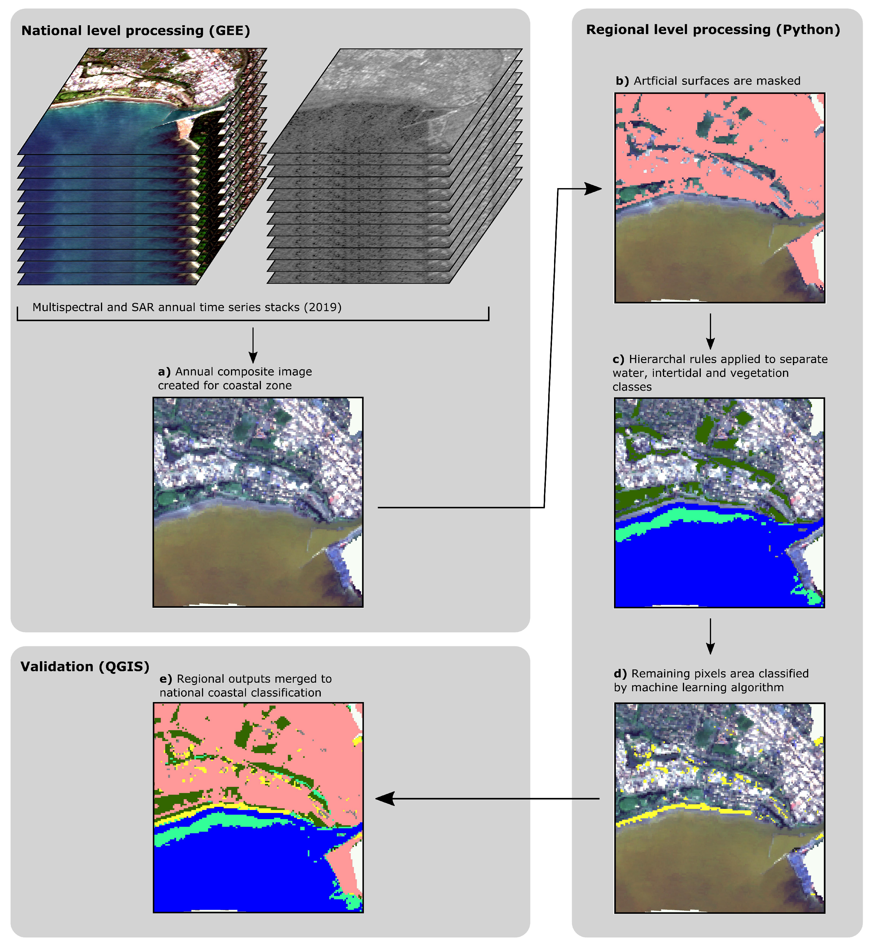
A mask was applied to remove pixels related to artificial surfaces to reduce confusion arising from mixed pixels (Figure 4). The mask was generated from vector data of New Zealand building footprints [61] and transport links [62] from 2019. Additionally, ports and industrial zones extracted from the New Zealand landcover database (LCDB), available from the Land Resource Information Systems Portal [63], were included in the mask. The LCDB is a national scale thematic landcover classification for New Zealand that is updated at five year intervals with accuracies exceeding 90% [64], but does not include coastal specific classes. It was derived using image processing and manual digitising techniques incorporating satellite imagery (SPOT 5 and Landsat) and aerial photos with a minimum mapping unit of one hectare. The most recent version was used in this study which was updated in summer 2018/19. All inputs were buffered by 20 m, dissolved and merged to form a single mask for artificial surfaces. Artificial surfaces were removed from the classification workflow but were still considered as a class to assess the ability of the mask to reduce confusion between sedimentary classes and built areas. Ancillary elevation data was used to remove most sections of cliffed coast, an threshold of 10 m was generated from national freely available 15 m resolution digital elevation model [65] which was resampled to 20 m resolution to match the composite images. Elevation data was not used in the classification workflow but was used to remove cliffed coast as the focus of this study was unconsolidated sections of the coast.
The first step of the classification framework was a set of hierarchal rules to separate spectrally heterogenous classes which included, water, intertidal and vegetation (Figure 5). The rule base was applied as spectrally heterogenous classes could be identified without the requirement for manually derived training data. Reducing the number of pixels to be classified via machine learning also improved computational efficiency as less classes required training. Automated Otsu thresholding [66] was applied to the 50th percentile MNDWI band to separate water and non-water pixels. To identify intertidal pixels contained in the water class, multi-level Otsu thresholding [67] was applied to the standard deviation MNDWI band as it was assumed that water pixels with high standard deviation indicated areas that were periodically submerged due to tidal influence. Non-water pixels were separated into vegetation and non-vegetation pixels with Otsu thresholding applied to the NDVI band. The remaining pixels were then classified using a random forest supervised machine learning classifier [68].

2.4. Developing Coastal Specific Training Data

National scale training data was required for the remaining classes to ensure that training was representative of all environments under investigation. To achieve this a training dataset, underpinned by the Landcover Database (LCDB), was manually derived based on the nomenclature developed in this study (Table 2). The LCDB was clipped to the coastal zone and any subclasses associated with vegetation, water and artificial areas were removed. The remaining classes (Sand/Gravel, Gravel/Rock and Estuarine water) were then used as a basis for developing training data for the remaining coastal classes. For each class, geometries were adjusted to ensure any boundaries did not cover multiple classes. This was performed manually in QGIS using high resolution aerial photos and commercial optical satellite imagery from 2019. The LCDB derives sedimentary classes by grain size. These were separated into bare rock, dark sand, gravel, light sand and supratidal sand. Intertidal was included in the training data to ensure that any intertidal pixels that had not been identified as water by the hierarchal rules were correctly classified. This provided a national training dataset, specific to the New Zealand coast, that was visually checked and included an estimation of the relative proportion of each class within the coastal zone to be identified by the machine learning classification.

2.5. Machine Learning Classification

Random forests was selected for the ability to provide accurate results working with high dimensional, multi-collinear data [69] which was important given the physical characteristics of the sedimentary coastal classes are similar. Area-proportional training obtains better results for classification trees compared with random sampling [70]. The national training dataset was masked by the area of remaining pixels to be classified and random proportional samples were selected that accounted for approximately 10% of the total pixels to be classified. The number of training samples per class were proportional to its coverage within the training dataset and was always greater than 2000 samples per class (Table 3). A total of 123,442 training samples were used to train the classifier. The number of estimators for the classifier (50) was identified using parameter grid search analysis. To assess the combination of SAR and optical data, two outputs were generated where one was trained using both S1 and S2 composite imagery and one trained just using S2 data.

2.6. Validation

2.6.1. Accuracy Assessment

The classification was validated using a point-based accuracy assessment generated from stratified random sampling using the classification. For each of the nine classes 2000 points was distributed at the national level for a total of 18,000 points. These were visually assessed against very high spatial resolution (less than 1 m) aerial photos and commercial satellite data acquired in 2019. Where such data was not available, high resolution (5 m) Planet satellite data was used from the Quarterly global mosaic for the first quarter of 2019 to correspond with the least cloudy conditions. Each point was buffered by 20 m to account for the classification resolution, to avoid bias, when manually assessing points against high resolution aerial photos and satellite data.
Points were ground-truthed using a custom QGIS plugin [27]. Accuracy scores were reported regionally and nationally. A confusion matrix was used to assess producers and users accuracy metrics. Quantity and allocation disagreement [71] was also calculated allowing for overall accuracy to be reported where the reference points were normalised by the area of each class detected and the number of samples per class, referred to as proportion correct. F-scores were also calculated for each class using producers and users accuracy as these metrics are representative of recall and precision [72]. F-scores were used to evaluate the accuracy of individual classes. The accuracy results from the combination of S1 and S2 data and just S2 were compared to evaluate the contribution of the SAR data to the accuracy of the classification.

2.6.2. Impact of Observation Frequency

When a greater the number of image acquisitions were used to derive composite imagery it has been shown to reduce errors in shoreline position [19]. The impact of the number of S2 images used to derive the multispectral composite image on classification accuracy was assessed. The number of image acquisitions (referred to as observations per pixel) used to develop the multispectral composite at each reference point in the accuracy assessment was calculated to assess whether there was relationship between correctly classified pixels and frequency of observations. Both surface reflectance and top-of-atmosphere collections were compared due to variation in the number of images in those collections. For each reference point, association between the number of observations at that given pixel and whether it had been correctly classified was assessed using point biserial correlation coefficient, a statistical tool to assess the relationship between categorical and continuous variables [73].

2.6.3. Comparison with Luijendijk et al. (2018) Classification

To assess the ability of the workflow to handle complex heterogeneous coastal environments at large scales the final output was compared against the sandy beaches classification developed by [24]. Luijendijk et al. [24] identified the world’s coasts as sandy or non-sandy by applying supervised machine learning classifier to S2 images with training data acquired from 100 km of Dutch coastline. The classification output was 97% accurate when validated against 100 km of beaches in the Netherlands and 96% accurate when checked against 50 international sites [24].
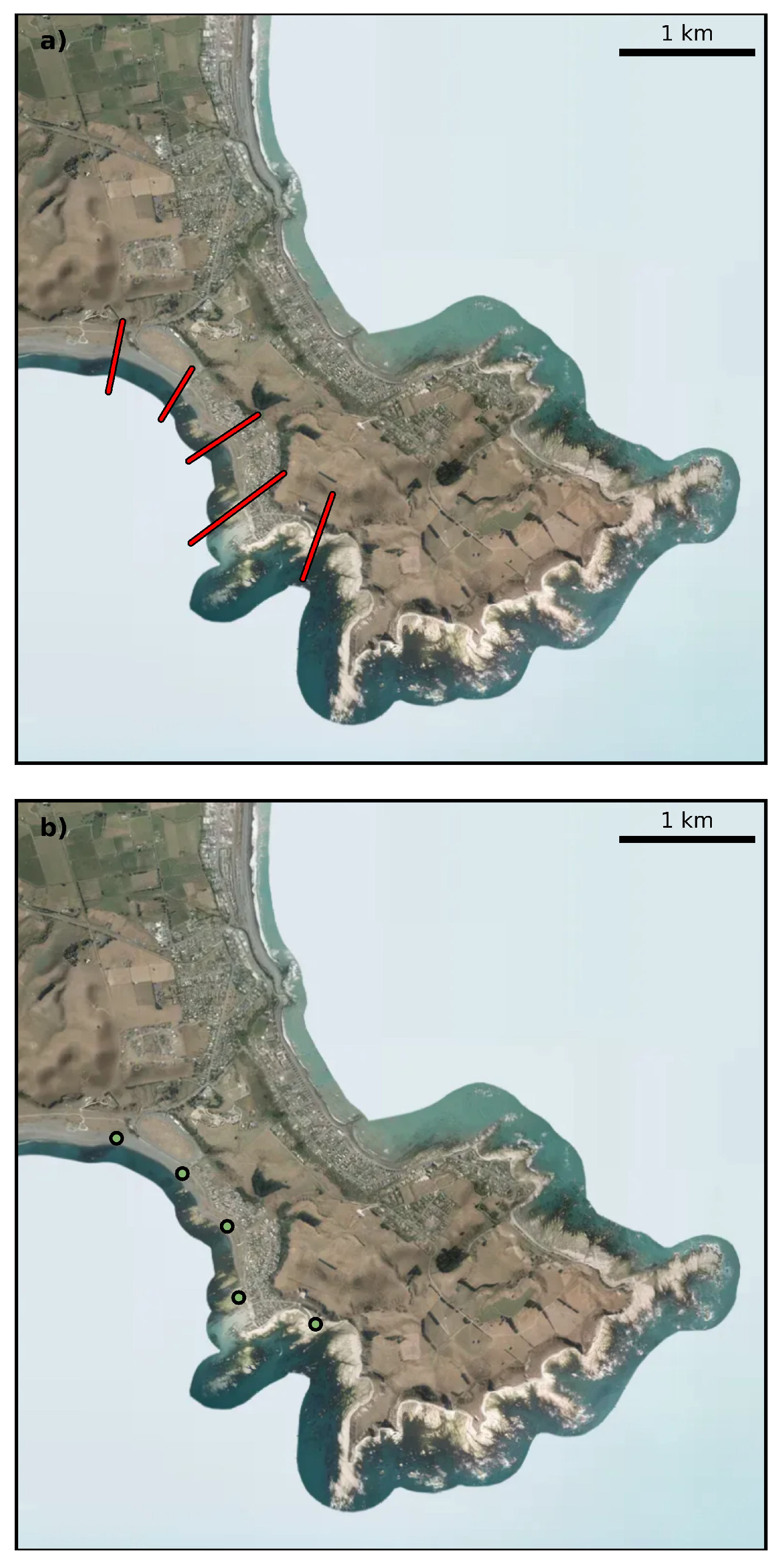
Points were generated around the New Zealand Coast at 50 km intervals. For each point, corresponding shoreline transects from [24] were identified. A further four transects, two either side of the initial transect, at 500 m intervals were identified providing five transects at 106 locations around the entire New Zealand coast (Figure 6). Both classifications were assessed against the high-resolution data and identified as either sand or non-sand using the same metrics as the point-based accuracy assessment.

3. Results

3.1. 2019 SAR and Multispectral Classification

A total of nine coastal landcover classes were classified for the whole of the New Zealand coastline, these included: water, intertidal areas, vegetation, artificial surfaces, light sand, dark sand, gravel, bare rock, and supratidal sand. Visual assessment indicated that the workflow identified coastal landcover types well (Figure 7).
Overall accuracies for the regional classifications varied from 76% (Southland) and 94% (Auckland). Overall accuracy was 86.38% with 99% probability the true value was between 85.38% and 87.08% based on the Wilson score interval [74] and the z-score was significant at p < 0.01 . A summary of the accuracy metrics are presented in Table 4.
In all regions (excluding Northland and Auckland), allocation disagreement was less than quantity disagreement, including nationally (0.0012 and 0.053, respectively). Higher quantity disagreement indicates extensive differences between classified and ground-truth reference points for each class and higher allocation disagreement implies there are differences in the spatial allocation of classes [75]. In this case, greater quantity disagreement suggests the area classified for some classes contains the majority of the disagreement. The overall proportion correct was high (93.6%) indicating the that workflow is effective at separating coastal specific classes for the New Zealand coast.
The highest omission errors were associated with the water class (0.0523) (Table 5). This was due to the misclassification of water as intertidal, particularly evident in the Southland region and along coastlines that are characterised by energetic wave conditions, which was evident at Piha and Gisborne (Figure 7).
The misclassification of water as intertidal corresponded with the highest commission errors evident for the intertidal class (0.0537) which was the worst performing class. However, intertidal zones were still well identified in estuaries which was highlighted at Nelson and Motueka (Figure 8).
The corresponding quantity disagreement indicates that the poor identification of the intertidal class contains the majority of disagreement within the classification. Sedimentary classes (light and dark sand and gravel) were well resolved with F-scores exceeding 0.82. Gravel had the lowest score (F-score = 0.82) which related to commission errors (0.0012) associated with misclassification of all other terrestrial classes. Light sand performed better (F-score = 0.85) but commission errors were also evident due to confusion amongst all other terrestrial classes. Omission errors for this class (0.0028) was associated predominantly with other sedimentary types. Dark sand performed best (F-score = 0.94).
Artificial surfaces had high accuracy (F-score = 0.92) indicating that by using a mask confusion between developed areas and sedimentary classes was reduced. High accuracy of the vegetation class (F-score = 0.94) also illustrates that the hierarchal rules were robust. Omission errors occurred for both classes where pixels were either excluded from the mask or omitted by the rules and passed to the machine learning workflow. In both cases most misclassified pixels were associated with light sand and gravel. The classification identified supratidal sand well (F-score = 0.85). Omission was greater than commission errors and related to the misclassification of sedimentary classes, predominantly gravel and light sand. Commission was associated with all other classes (excluding water), and occurred most often for bare rock.
The bare rock class also performed well (F1-score = 0.90). Omission was related to confusion with sedimentary and supratidal sand. Commission errors were present for all other classes (excluding water), with the majority of misclassification as artificial surfaces that were omitted from the mask.

3.2. SAR Contribution

An iteration of the classification was performed using the S2 data alone. Overall accuracy was 71.20 ± 0.87%, based on the same set of reference data (Table 6). Incorporating SAR data led to increases in overall accuracy of 14.4% and 3.7% in proportion correct. Comparisons of F1-scores showed improvement in detection of all classes that were not classified by the hierarchal rules (bare rock, dark sand, gravel, light sand, and supratidal sand) (Figure 9).
The greatest differences were for the bare rock class (∼50%) where confusion between all other classes was improved, particularly the intertidal class. Where only optical data was used, ∼60% of reference points identified as bare rock were classified intertidal. Including SAR data improved the detection dark sand and gravel by ∼16%.
Improvements for the light sand class were the smallest (∼10%). Classification of the supratidal sand class was also improved by ∼14%, by enhancing separation between other sedimentary classes and the intertidal class. Without SAR data, intertidal pixels missed by the hierarchal rules were poorly resolved and misclassified as terrestrial classes. In all cases, the use of SAR reduced misclassification of the intertidal class. This indicates the importance of SAR data in accurate detection of heterogeneous coastal land cover types and suggests that combining multispectral and SAR satellite earth observation data achieves accuracies required for robust pixel-based change detection at the coast.

3.3. Frequency of Observations

Variation in the number of clear observations used to derive the multispectral composite was high. The maximum number of observations for both collections exceeded 200 where there is overlap of S2 tiles. The minimum number of observations was in Southland where cloud cover was high and the number of available images throughout the year was also low, mean observations for top-of-atmosphere was 45 and surface reflectance was 36.
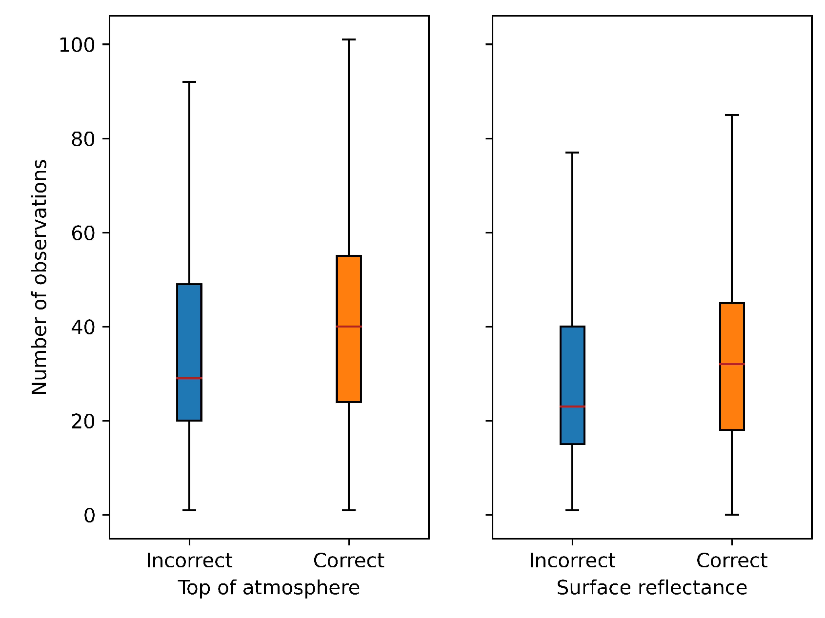
The correlation coefficient, r p b for observation frequency against top-of-atmosphere and surface reflectance collections was 0.106 (p = 3.89) and 0.102 (p = 3.64), respectively. Slight positive correlation suggest that an increased number of clear observations per pixel led to greater accuracy of the classification, but this was not statistically significant across all classes (Figure 10). For the worst performing class (intertidal), r p b was calculated to see if there was a statistically significant association between misclassified pixels and the frequency of observations. For top-of-atmosphere and surface reflectance, r p b was 0.937 (p = 0.001) and 0.892 (p= 0.002), respectively, indicating a statistically significant relationship where correctly classified pixels are associated with a greater number of observations.
It is clear that the range of observations across the New Zealand land mass is large, owing to acquisition parameters, tile overlap, and cloud cover. Errors in the worst performing class present strong correlation with the number of clear observations used to derive the composite pixel values; however, overall association between correctly classified pixels across all classes is small.

4. Discussion

This study presents a new methodology for coastal landcover classification using a combination of public multispectral and SAR satellite data, enabling the first national-scale pixel-based coastal specific landcover classification for the open coast of New Zealand. This has been validated to provide an empirical assessment of accuracy that is significant at p < 0.01 and results indicate that coastal land cover types have been mapped with accuracies exceeding 90%. The methodology is automated and scalable, combining a novel approach of hierarchal rules to separate spectrally distinct classes and machine learning to classify heterogeneous land cover types. This was implemented in two steps, first leveraging GEE to derive composite imagery, and then using local computing resources with 8-cores and 16 GB of RAM to perform the classification. This means it can be deployed via a standard computer with good internet and does not require access to high-performance-computing resources. Empirical validation of the classification output indicates that the workflow is robust, detecting sedimentary landcover types by dominant lithologies including other classes that are important in the role of evolution at the coast (e.g., intertidal areas, supratidal sand, and vegetation) (Figure 7).

4.1. Comparison with Other Analyses of Sandy Coast in New Zealand

A total of 530 points were visually assessed to determine whether they were sand or non-sand in the high-resolution reference data, the classification output and corresponding transects derived from the approach developed by [24]. The workflow presented in this study was 91 ± 3% at 99% probability. In comparison 62 ± 5% of the transects derived by [24] were correctly identified as sandy. This improvement in accuracy highlights the robustness of the workflow, stressing the need for comprehensive local training data. It is important that classification workflows must be developed with appropriate training data that is representative of the environment under investigation. This also further highlights the benefit of a combination of SAR and multispectral data for physically heterogeneous environments and suggests it could be appropriate for other varied coastal settings around the world.
To date, the use of per-pixel remote sensing techniques at the coast have focused on separating land and water [15], improving estimates of the IW shoreline position [13], and detecting the seaward vegetation edge to extract beach width [33]. These approaches provide objective repeatable methods for assessing trends in shoreline position, but sources of uncertainty mean there is substantial noise contained in the position of the IW boundary. Extracting meaningful information in the context of long-term coastal change can be challenging. Short-term processes driving instantaneous IW shoreline response initiate long-term change over prolonged timescales [76], but medium/long term changes may not be governed by these individual processes [11]. Increasing sediment availability, for instance, can cause a system to switch from erosive to accretive. Assessing long-term variations through the analysis of change rates in the IW position will not capture all functions of coastal change and is subject to environmental uncertainty.
Pixel-based techniques provide the opportunity to assess change across the entire coastal zone rather than condensing information to focus on single shoreline proxies. Accurate identification of land cover types is an initial step in per-pixel change detection, working toward assessing change across the coastal zone rather than just the change in the position of the shoreline to reduce environmental uncertainty in change analysis. Sediment supply, is a fundamental driver of coastal change and evolution at long time instances [77] and this method presents the opportunity to assess changes in sediment supply. For example, decreases in supratidal sand could be a leading indicator that sediment delivery is diminishing for a given beach. Detection and further separation of the vegetation class could also provide a high level overview of vegetation at the coast to better understand how this landcover is changing and the implications this has in the context of coastal evolution. This workflow presents the opportunity to investigate changes by sediment type around the New Zealand coast including other coastal specific classes.

4.2. Impact of Observation Frequency

Correlation between correctly identified pixels and observation frequency was evident for all landcover types but was statistically insignificant across all classes. Image compositing techniques have been used to alleviate errors associated with cloud cover and wave run-up when extracting shorelines from earth observation data [19,24]. This has been found to reduce temporal resolution and deemed inappropriate for shoreline detection in meso/macro-tidal environments [13] but, it was found that offset errors in satellite derived shorelines decreased when the number of days included in a composite image window increased, suggesting that the technique was suitable for assessing inter-annual trends [19]. Association between correctly classified pixels and the frequency of observations support this and indicate composite images are appropriate for assessing long-term inter-annual coastal change via pixel-based remote sensing techniques. Compositing was an important part of this approach, combining S1 and S2 data to classify a region at a single time instance could be challenging due to differences in the time of acquisition. Assessing change at shorter timescales (e.g., episodic/event) may therefore be limited. Further work is required to investigate the suitability of pixel-based compositing techniques for coastal change occurring at intra-annual time scales and shorter.

4.3. The Importance of SAR for Coastal Landcover Classification

This is among one of the first studies that combines multispectral and SAR satellite data for specific coastal landcover mapping at national scale. The accuracy of the classification was greater for all classes when a combination of SAR and optical data were used, increasing overall accuracy by ∼ 15% and improving detection of all sedimentary classes (Figure 9). Improvements in the detection of sedimentary classes was 10–50% and all classes were better identified. Most strikingly, ∼ 60% more reference points identified as bare rock were correctly classified when SAR and multispectral data were used in the classification workflow. The noteworthy improvement in detection of rock surfaces could find useful application in global efforts to map the distribution of cliffed coastlines [78] and anticipate their vulnerability to climate change, for example, [79]. This is likely due to the spectral similarities of sedimentary land cover at the New Zealand coast. SAR was incorporated to provide information about the physical properties of classes under investigation. It is clear that SAR data is instrumental in developing accurate coastal landcover products where environments are physically complex. These results indicate that using a combination of optical and SAR data provides significant improvements to a coastal specific landcover classification. Such a workflow ensures accuracies high enough for robust high-level change analyses along the New Zealand coastline at inter-annual timescales utilising per-pixel techniques to provide insights beyond mapping a single shoreline proxy using remote sensing satellite data.
Map-to-image change detection techniques have been demonstrated to be suitable for monitoring change in mangrove extent at global scales, offering advantages over image-to-image and map-to-map techniques and the ability to use earth observation data collected from a range of sensors including multispectral and SAR data [27,80]. This means a greater volume of data can be used to assess change over longer time instances by incorporating multispectral data from the Landsat archive without the requirement for SAR where it is not available. These are yet to be applied in assessments of coastal change using earth observation data and should be investigated. Information gained from such an approach can be used to inform coastal management practises, rather than decision making occurring based solely on IW shoreline change analysis.

5. Conclusions

A coastal landcover cover classification was developed for the New Zealand coastline, mapping coastal regions by dominant sediment types using a combination of public multispectral and synthetic-aperture-radar data. Overall accuracies exceeded 90% when validation data was normalised by class area. The classification workflow was developed using open-source software and code, allowing it to be applied elsewhere. Compared with previous approaches, accuracy was 30% greater overall, highlighting the importance of accounting for the complexity of coastal environments. Accuracy was enhanced for coastal specific sedimentary classes (10–50%) by incorporating a combination of SAR and multispectral earth observation sensor types, achieving robust results. This approach can be developed further with change-detection analysis offering insights to long-term land cover change at the coast in New Zealand and elsewhere, to provide decision-makers and coastal scientists with information to better prepare for future change at the coast.

Author Contributions

Conceptualization, B.C., M.F. and M.D.; methodology, B.C.; software, B.C.; validation, B.C.; investigation, B.C.; resources, B.C.; data curation, B.C.; writing—original draft preparation, B.C.; writing—review and editing, B.C., M.F. and M.D.; visualization, B.C.; supervision, M.F. and M.D. All authors have read and agreed to the published version of the manuscript.

Funding

This research was funded by the Resilience to Nature’s Challenges National Science Challenge through the New Zealand Ministry of Business, Innovation and Employment as part of the Coastal Programme under the ‘New Zealand’s Changing Coastline’ project (NSCIC C005250).

Data Availability Statement

The coastal classification is available to view as a GEE app (https://bcol845.users.earthengine.app/view/nzcc-2019, accessed on 22 July 2022) and code used to generate the product is available on Github under a GPL-3.0 license (https://github.com/bmcollings/coastal-landcover-classification, accessed on 8 July 2022).

Acknowledgments

This research was supported by use of the Nectar Research Cloud and by the University of Auckland. The Nectar Research Cloud is a collaborative Australian research platform supported by the NCRIS-funded Australian Research Data Commons (ARDC).

Conflicts of Interest

The authors declare no conflict of interest.

Abbreviations

The following abbreviations are used in this manuscript:
AWEIAutomated Water Extraction Index
GEEGoogle Earth Engine
GRDGround Range Detected
H s Significant wave height
IWInstantaneous waterline
LCDBLandcover Database
LiDARLight detecting and ranging
MNDWIModified Normalised Difference Water Index
NDVINormalised Difference Vegetation Index
NDWINormalised Difference Water Index
NeCTARAustralian National eResearch Collaboration Tools and Resources
RMSERoot mean square error
RSGISLIBRemote Sensing and GIS libraries
S1Sentinel-1
S2Sentinel-2
SARSynthetic Aperture Radar
SRSurface reflectance
TOATop of Atmosphere

References

  1. Revell, D.L.; Battalio, R.; Spear, B.; Ruggiero, P.; Vandever, J. A methodology for predicting future coastal hazards due to sea-level rise on the California Coast. Clim. Chang. 2011, 109, 251–276. [Google Scholar] [CrossRef]
  2. Lawrence, J.; Sullivan, F.; Lash, A.; Ide, G.; Cameron, C.; McGlinchey, L. Adapting to changing climate risk by local government in New Zealand: Institutional practice barriers and enablers. Local Environ. 2015, 20, 298–320. [Google Scholar] [CrossRef]
  3. Purkis, S.J.; Klemas, V.V. Remote Sensing and Global Environmental Change; John Wiley & Sons: Hoboken, NJ, USA, 2013. [Google Scholar] [CrossRef]
  4. Boak, E.H.; Turner, I.L. Shoreline definition and detection: A review. J. Coast. Res. 2005, 21, 688–703. [Google Scholar] [CrossRef]
  5. Toure, S.; Diop, O.; Kpalma, K.; Maiga, A.S. Shoreline detection using optical remote sensing: A review. ISPRS Int. J. Geo-Inf. 2019, 8, 75. [Google Scholar] [CrossRef]
  6. Ford, M. Shoreline changes interpreted from multi-temporal aerial photographs and high resolution satellite images: Wotje Atoll, Marshall Islands. Remote Sens. Environ. 2013, 135, 130–140. [Google Scholar] [CrossRef]
  7. Blue, B.; Kench, P.S. Multi-decadal shoreline change and beach connectivity in a high-energy sand system. N. Z. J. Mar. Freshw. Res. 2017, 51, 406–426. [Google Scholar] [CrossRef]
  8. Splinter, K.; Harley, M.; Turner, I. Remote Sensing Is Changing Our View of the Coast: Insights from 40 Years of Monitoring at Narrabeen-Collaroy, Australia. Remote Sens. 2018, 10, 1744. [Google Scholar] [CrossRef]
  9. Harley, M.D.; Turner, I.L.; Kinsela, M.A.; Middleton, J.H.; Mumford, P.J.; Splinter, K.D.; Phillips, M.S.; Simmons, J.A.; Hanslow, D.J.; Short, A.D. Extreme coastal erosion enhanced by anomalous extratropical storm wave direction. Sci. Rep. 2017, 7, 6033. [Google Scholar] [CrossRef]
  10. Castelle, B.; Guillot, B.; Marieu, V.; Chaumillon, E.; Hanquiez, V.; Bujan, S.; Poppeschi, C. Spatial and temporal patterns of shoreline change of a 280-km high-energy disrupted sandy coast from 1950 to 2014: SW France. Estuar. Coast. Shelf Sci. 2018, 200, 212–223. [Google Scholar] [CrossRef]
  11. Bryan, K.R.; Kench, P.S.; Hart, D.E. Multi-decadal coastal change in New Zealand: Evidence, mechanisms and implications. N. Z. Geogr. 2008, 64, 117–128. [Google Scholar] [CrossRef]
  12. Gorelick, N.; Hancher, M.; Dixon, M.; Ilyushchenko, S.; Thau, D.; Moore, R. Google Earth Engine: Planetary-scale geospatial analysis for everyone. Remote Sens. Environ. 2017, 202, 18–27. [Google Scholar] [CrossRef]
  13. Vos, K.; Harley, M.D.; Splinter, K.D.; Simmons, J.A.; Turner, I.L. Sub-annual to multi-decadal shoreline variability from publicly available satellite imagery. Coast. Eng. 2019, 150, 160–174. [Google Scholar] [CrossRef]
  14. Pardo-Pascual, J.E.; Almonacid-Caballer, J.; Ruiz, L.A.; Palomar-Vázquez, J. Automatic extraction of shorelines from Landsat TM and ETM+ multi-temporal images with subpixel precision. Remote Sens. Environ. 2012, 123, 1–11. [Google Scholar] [CrossRef]
  15. Xu, N. Detecting Coastline Change with All Available Landsat Data over 1986–2015: A Case Study for the State of Texas, USA. Atmosphere 2018, 9, 107. [Google Scholar] [CrossRef]
  16. Liu, Q.; Trinder, J.; Turner, I.L. Automatic super-resolution shoreline change monitoring using Landsat archival data: A case study at Narrabeen–Collaroy Beach, Australia. J. Appl. Remote Sens. 2017, 11, 16036. [Google Scholar] [CrossRef]
  17. Mentaschi, L.; Vousdoukas, M.I.; Pekel, J.F.; Voukouvalas, E.; Feyen, L. Global long-term observations of coastal erosion and accretion. Sci. Rep. 2018, 8, 12876. [Google Scholar] [CrossRef]
  18. Almonacid-Caballer, J.; Sánchez-García, E.; Pardo-Pascual, J.E.; Balaguer-Beser, A.A.; Palomar-Vázquez, J. Evaluation of annual mean shoreline position deduced from Landsat imagery as a mid-term coastal evolution indicator. Mar. Geol. 2016, 372, 79–88. [Google Scholar] [CrossRef]
  19. Hagenaars, G.; de Vries, S.; Luijendijk, A.P.; de Boer, W.P.; Reniers, A.J.H.M. On the accuracy of automated shoreline detection derived from satellite imagery: A case study of the sand motor mega-scale nourishment. Coast. Eng. 2018, 133, 113–125. [Google Scholar] [CrossRef]
  20. Mcallister, E.; Payo, A.; Novellino, A.; Dolphin, T.; Medina-Lopez, E. Multispectral satellite imagery and machine learning for the extraction of shoreline indicators. Coast. Eng. 2022, 174, 104102. [Google Scholar] [CrossRef]
  21. U.S. Geological Survey. Landsat Collection 1 Level 1 Product Definition; Technical Report; USGS: Reston, VA, USA, 2019. Available online: https://www.usgs.gov/media/files/landsat-collection-1-level-1-product-definition (accessed on 27 April 2022).
  22. Liu, Y.; Huang, H.; Qiu, Z.; Fan, J. Detecting coastline change from satellite images based on beach slope estimation in a tidal flat. Int. J. Appl. Earth Obs. Geoinf. 2013, 23, 165–176. [Google Scholar] [CrossRef]
  23. Castelle, B.; Masselink, G.; Scott, T.; Stokes, C.; Konstantinou, A.; Marieu, V.; Bujan, S. Satellite-derived shoreline detection at a high-energy meso-macrotidal beach. Geomorphology 2021, 383, 107707. [Google Scholar] [CrossRef]
  24. Luijendijk, A.; Hagenaars, G.; Ranasinghe, R.; Baart, F.; Donchyts, G.; Aarninkhof, S. The State of the World’s Beaches. Sci. Rep. 2018, 8, 6641. [Google Scholar] [CrossRef] [PubMed]
  25. Bishop-Taylor, R.; Nanson, R.; Sagar, S.; Lymburner, L. Mapping Australia’s dynamic coastline at mean sea level using three decades of Landsat imagery. Remote Sens. Environ. 2021, 267, 112734. [Google Scholar] [CrossRef]
  26. Zhu, Z. Change detection using landsat time series: A review of frequencies, preprocessing, algorithms, and applications. ISPRS J. Photogramm. Remote Sens. 2017, 130, 370–384. [Google Scholar] [CrossRef]
  27. Bunting, P.; Rosenqvist, A.; Lucas, R.M.; Rebelo, L.M.; Hilarides, L.; Thomas, N.; Hardy, A.; Itoh, T.; Shimada, M.; Finlayson, C.M. The global mangrove watch—A new 2010 global baseline of mangrove extent. Remote Sens. 2018, 10, 1669. [Google Scholar] [CrossRef]
  28. Donchyts, G.; Baart, F.; Winsemius, H.; Gorelick, N.; Kwadijk, J.; Van De Giesen, N. Earth’s surface water change over the past 30 years. Nat. Clim. Chang. 2016, 6, 810–813. [Google Scholar] [CrossRef]
  29. Hansen, M.C.; Stehman, S.V.; Potapov, P.V. Quantification of global gross forest cover loss. Proc. Natl. Acad. Sci. USA 2010, 107, 8650–8655. [Google Scholar] [CrossRef]
  30. Fitton, J.M.; Rennie, A.F.; Hansom, J.D.; Muir, F.M. Remotely sensed mapping of the intertidal zone: A Sentinel-2 and Google Earth Engine methodology. Remote Sens. Appl. Soc. Environ. 2021, 22, 100499. [Google Scholar] [CrossRef]
  31. Bernier, J.C.; Miselis, J.L.; Plant, N.G.; Zambrano Bigiarini, F.; Lu, B.; Smith, K.E.L.; Manuel Álvarez-Martínez, J.; Filipponi, F.; Niculescu, S.; Xia, J.; et al. Satellite-Derived Barrier Response and Recovery Following Natural and Anthropogenic Perturbations, Northern Chandeleur Islands, Louisiana. Remote Sens. 2021, 13, 3779. [Google Scholar] [CrossRef]
  32. Zinnert, J.C.; Via, S.M.; Nettleton, B.P.; Tuley, P.A.; Moore, L.J.; Stallins, J.A. Connectivity in coastal systems: Barrier island vegetation influences upland migration in a changing climate. Glob. Chang. Biol. 2019, 25, 2419–2430. [Google Scholar] [CrossRef]
  33. Latella, M.; Luijendijk, A.; Moreno-Rodenas, A.M.; Camporeale, C. Satellite image processing for the coarse-scale investigation of sandy coastal areas. Remote Sens. 2021, 13, 4613. [Google Scholar] [CrossRef]
  34. Kench, P.S.; Bryan, K.R.; Hart, D.E.; Kennedy, D.M.; Hilton, M.J. A commentary on coastal research in New Zealand universities. N. Z. Geogr. 2008, 64, 93–104. [Google Scholar] [CrossRef]
  35. Nicol, A.; Seebeck, H.; Wallace, L. Quaternary Tectonics of New Zealand. In Landscape and Quaternary Environmental Change in New Zealand; Atlantis Press: Amsterdam, The Netherlands, 2017; pp. 1–34. [Google Scholar] [CrossRef]
  36. Rouse, H.; Nichol, S.; Goff, J. Introduction to the New Zealand coast. In The New Zealand Coast: Te Tai o Aoteroa, 1st ed.; Goff, J.R., Nichol, S.L., Rouse, H.L., Eds.; Dunmore Press: Palmerston North, New Zealand, 2003; pp. 9–25. [Google Scholar]
  37. Komar, P.D. Shoreline evolution and management of Hawke’s Bay, New Zealand: Tectonics, coastal processes, and human impacts. J. Coast. Res. 2010, 26, 143–156. [Google Scholar] [CrossRef]
  38. Clark, K.J.; Nissen, E.K.; Howarth, J.D.; Hamling, I.J.; Mountjoy, J.J.; Ries, W.F.; Jones, K.; Goldstien, S.; Cochran, U.A.; Villamor, P.; et al. Highly variable coastal deformation in the 2016 MW7.8 Kaikōura earthquake reflects rupture complexity along a transpressional plate boundary. Earth Planet. Sci. Lett. 2017, 474, 334–344. [Google Scholar] [CrossRef]
  39. Hamill, P.F.; Ballance, P.F. Heavy mineral rich beach sands of the waitakere coast, Auckland, New Zealand. N. Z. J. Geol. Geophys. 1985, 28, 503–511. [Google Scholar] [CrossRef]
  40. Carter, L.; Manighetti, B.; Elliot, M.; Trustrum, N.; Gomez, B. Source, sea level and circulation effects on the sediment flux to the deep ocean over the past 15 ka off eastern New Zealand. Glob. Planet. Chang. 2002, 33, 339–355. [Google Scholar] [CrossRef]
  41. Schofield, J.C. Coastal sands of Northland and Auckland. N. Z. J. Geol. Geophys. 1970, 13, 767–824. [Google Scholar] [CrossRef]
  42. Albuquerque, J.; Antolínez, J.A.A.; Gorman, R.M.; Méndez, F.J.; Coco, G. Seas and swells throughout New Zealand: A new partitioned hindcast. Ocean Model. 2021, 168, 101897. [Google Scholar] [CrossRef]
  43. Rueda, A.; Cagigal, L.; Antolínez, J.A.; Albuquerque, J.C.; Castanedo, S.; Coco, G.; Méndez, F.J. Marine climate variability based on weather patterns for a complicated island setting: The New Zealand case. Int. J. Climatol. 2019, 39, 1777–1786. [Google Scholar] [CrossRef]
  44. Coggins, J.H.; Parsons, S.; Schiel, D. An assessment of the ocean wave climate of New Zealand as represented in Kidson’s synoptic types. Int. J. Climatol. 2016, 36, 2481–2496. [Google Scholar] [CrossRef]
  45. Lange, W.D.; Bell, R.; Gorman, R.; Reid, S. Physical oceanography of New Zealand waters. In The New Zealand Coast: Te Tai o Aoteroa, 1st ed.; Goff, J., Nichol, S., Rouse, H., Eds.; Dunmore Press with Whitireia Publishing and Daphne Brasell Associates: Palmerston North, New Zealand, 2003; pp. 59–78. [Google Scholar]
  46. Brander, R.W.; Osborne, P.D.; Parnell, K. High-energy beach and nearshore processes. In The New Zealand Coast: Te Tai o Aoteroa, 1st ed.; Goff, J., Nichol, S., Rouse, H., Eds.; Dunmore Press: Palmerston North, New Zealand, 2003; pp. 119–142. [Google Scholar]
  47. Main-Knorn, M.; Pflug, B.; Louis, J.; Debaecker, V.; Müller-Wilm, U.; Gascon, F. Sen2Cor for Sentinel-2. In Image and Signal Processing for Remote Sensing XXIII; SPIE: Warsaw, Poland, 2017; Volume 10427, pp. 37–48. [Google Scholar] [CrossRef]
  48. Filipponi, F. Sentinel-1 GRD Preprocessing Workflow. Proceedings 2019, 18, 11. [Google Scholar] [CrossRef]
  49. [dataset] Land Information New Zealand. New Zealand Coastline-Mean High Water. 2021. Available online: https://data.linz.govt.nz/layer/105085-nz-coastline-mean-high-water/ (accessed on 1 October 2021).
  50. Zhu, Z.; Woodcock, C.E. Continuous change detection and classification of land cover using all available Landsat data. Remote Sens. Environ. 2014, 144, 152–171. [Google Scholar] [CrossRef]
  51. Hisabayashi, M.; Rogan, J.; Elmes, A. Quantifying shoreline change in Funafuti Atoll, Tuvalu using a time series of Quickbird, Worldview and Landsat data. GIScience Remote Sens. 2017, 55, 307–330. [Google Scholar] [CrossRef]
  52. Holdaway, A.; Ford, M.; Owen, S. Global-scale changes in the area of atoll islands during the 21st century. Anthropocene 2021, 33. [Google Scholar] [CrossRef]
  53. Donchyts, G.; Schellekens, J.; Winsemius, H.; Eisemann, E.; van de Giesen, N. A 30 m resolution surfacewater mask including estimation of positional and thematic differences using landsat 8, SRTM and OPenStreetMap: A case study in the Murray-Darling basin, Australia. Remote Sens. 2016, 8, 386. [Google Scholar] [CrossRef]
  54. Kriegler, F.; Malila, W.; Nalepka, R.; Richardson, W. Preprocessing transformations and their effect on multispectral recognition. In Proceedings of the 6th International Symposium on Remote Sensing of Environment, Ann Arbor, MI, USA, 13–16 October 1969; pp. 97–131. [Google Scholar]
  55. McFeeters, S.K. The use of the Normalized Difference Water Index (NDWI) in the delineation of open water features. Int. J. Remote Sens. 1996, 17, 1425–1432. [Google Scholar] [CrossRef]
  56. Xu, H. Modification of normalised difference water index (NDWI) to enhance open water features in remotely sensed imagery. Int. J. Remote Sens. 2006, 27, 3025–3033. [Google Scholar] [CrossRef]
  57. Feyisa, G.L.; Meilby, H.; Fensholt, R.; Proud, S.R. Automated Water Extraction Index: A new technique for surface water mapping using Landsat imagery. Remote Sens. Environ. 2014, 140, 23–35. [Google Scholar] [CrossRef]
  58. Vandebroek, E.; Lindenbergh, R.; van Leijen, F.; de Schipper, M.; de Vries, S.; Hanssen, R. Semi-automated monitoring of a mega-scale beach nourishment using high-resolution terraSAR-X satellite data. Remote Sens. 2017, 9, 653. [Google Scholar] [CrossRef]
  59. European Space Agency. Sentinel-1 SAR User Guide; Technical Report; ESA: Paris, France, 2015; Available online: https://sentinel.esa.int/web/sentinel/user-guides/sentinel-1-sar (accessed on 1 November 2021).
  60. Bunting, P.; Clewley, D.; Lucas, R.M.; Gillingham, S. The Remote Sensing and GIS Software Library (RSGISLib). Comput. Geosci. 2014, 62, 216–226. [Google Scholar] [CrossRef]
  61. [dataset] Land Information New Zealand. NZ Road Centrelines (Topo, 1:50k). 2022. Available online: https://data.linz.govt.nz/layer/50329-nz-road-centrelines-topo-150k/ (accessed on 8 February 2022).
  62. [dataset] Land Information New Zealand. NZ Building Outlines. 2021. Available online: https://data.linz.govt.nz/layer/101290-nz-building-outlines/ (accessed on 8 February 2022).
  63. [dataset] Landcare Research. LCDB v5.0-Land Cover Database version 5.0, Mainland, New Zealand. 2021. Available online: https://lris.scinfo.org.nz/layer/104400-lcdb-v50-land-cover-database-version-50-mainland-new-zealand/ (accessed on 1 December 2021).
  64. Dymond, J.R.; Shepherd, J.D.; Newsome, P.F.; Belliss, S. Estimating change in areas of indigenous vegetation cover in New Zealand from the New Zealand Land Cover Database (LCDB). N. Z. J. Ecol. 2017, 41, 56–64. [Google Scholar] [CrossRef]
  65. Columbus, J.; Sirguey, P.; Tenzer, R. A free, fully assessed 15-m DEM for New Zealand. Surv. Q. 2011, 66, 16–19. [Google Scholar]
  66. Otsu, N. A Threshold Selection Method from Gray-Level Histograms. IEEE Trans. Geosci. Remote Sens. 1979, 9, 62–66. [Google Scholar] [CrossRef]
  67. Liao, P.S.; Chen, T.S.; Chung, P.C. A fast algorithm for multilevel thresholding. J. Inf. Sci. Eng. 2001, 17, 713–727. [Google Scholar] [CrossRef]
  68. Breiman, L. Random Forests. Mach. Learn. 2001, 45, 5–32. [Google Scholar] [CrossRef]
  69. Rodriguez-Galiano, V.F.; Ghimire, B.; Rogan, J.; Chica-Olmo, M.; Rigol-Sanchez, J.P. An assessment of the effectiveness of a random forest classifier for land-cover classification. ISPRS J. Photogramm. Remote Sens. 2012, 67, 93–104. [Google Scholar] [CrossRef]
  70. Colditz, R. An Evaluation of Different Training Sample Allocation Schemes for Discrete and Continuous Land Cover Classification Using Decision Tree-Based Algorithms. Remote Sens. 2015, 7, 9655–9681. [Google Scholar] [CrossRef]
  71. Pontius, R.G.; Millones, M. Death to Kappa: Birth of quantity disagreement and allocation disagreement for accuracy assessment. Int. J. Remote Sens. 2011, 32, 4407–4429. [Google Scholar] [CrossRef]
  72. Modica, G.; De Luca, G.; Messina, G.; Praticò, S. Comparison and assessment of different object-based classifications using machine learning algorithms and UAVs multispectral imagery: A case study in a citrus orchard and an onion crop. Eur. J. Remote Sens. 2021, 54, 431–460. [Google Scholar] [CrossRef]
  73. Tate, R.F. Correlation between a Discrete and a Continuous Variable. Point-Biserial Correlation. Ann. Math. Stat. 1954, 25, 603–607. [Google Scholar] [CrossRef]
  74. Wilson, E.B. Probable Inference, the Law of Succession, and Statistical Inference. J. Am. Stat. Assoc. 1927, 22, 209. [Google Scholar] [CrossRef]
  75. Warrens, M.J. Properties of the quantity disagreement and the allocation disagreement. Int. J. Remote Sens. 2015, 36, 1439–1446. [Google Scholar] [CrossRef]
  76. Wright, L.D.; Thom, B.G. Coastal depositional landforms. Prog. Phys. Geogr. Earth Environ. 1977, 1, 412–459. [Google Scholar] [CrossRef]
  77. Masselink, G.; Hughes, M.; Knight, J. Introduction to Coastal Process and Geomorphology, 2nd ed.; Routledge: London, UK, 2011. [Google Scholar] [CrossRef]
  78. Young, A.P.; Carilli, J.E. Global distribution of coastal cliffs. Earth Surf. Process. Landforms 2019, 44, 1309–1316. [Google Scholar] [CrossRef]
  79. Dickson, M.E.; Walkden, M.J.; Hall, J.W. Systemic impacts of climate change on an eroding coastal region over the twenty-first century. Clim. Chang. 2007, 84, 141–166. [Google Scholar] [CrossRef]
  80. Thomas, N.; Bunting, P.; Lucas, R.; Hardy, A.; Rosenqvist, A.; Fatoyinbo, T. Mapping mangrove extent and change: A globally applicable approach. Remote Sens. 2018, 10, 1466. [Google Scholar] [CrossRef] [Green Version]
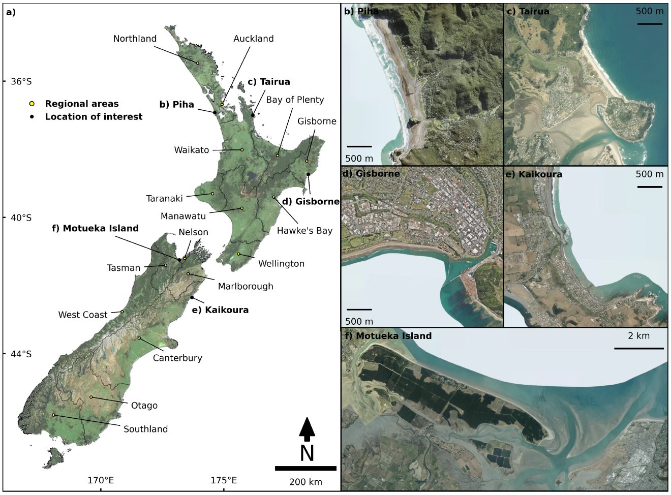
Figure 1. (a) New Zealand regional council areas and locations of interest indicating the diversity of the coast. (b)Piha beach in Auckland region. (c) Tairua in Waikato region. (d) Gisborne city in Gisborne region. (e) Kaikoura in Canterbury region. (f) Nelson and Motueka Island in Nelson region.
Remotesensing 14 04827 g001
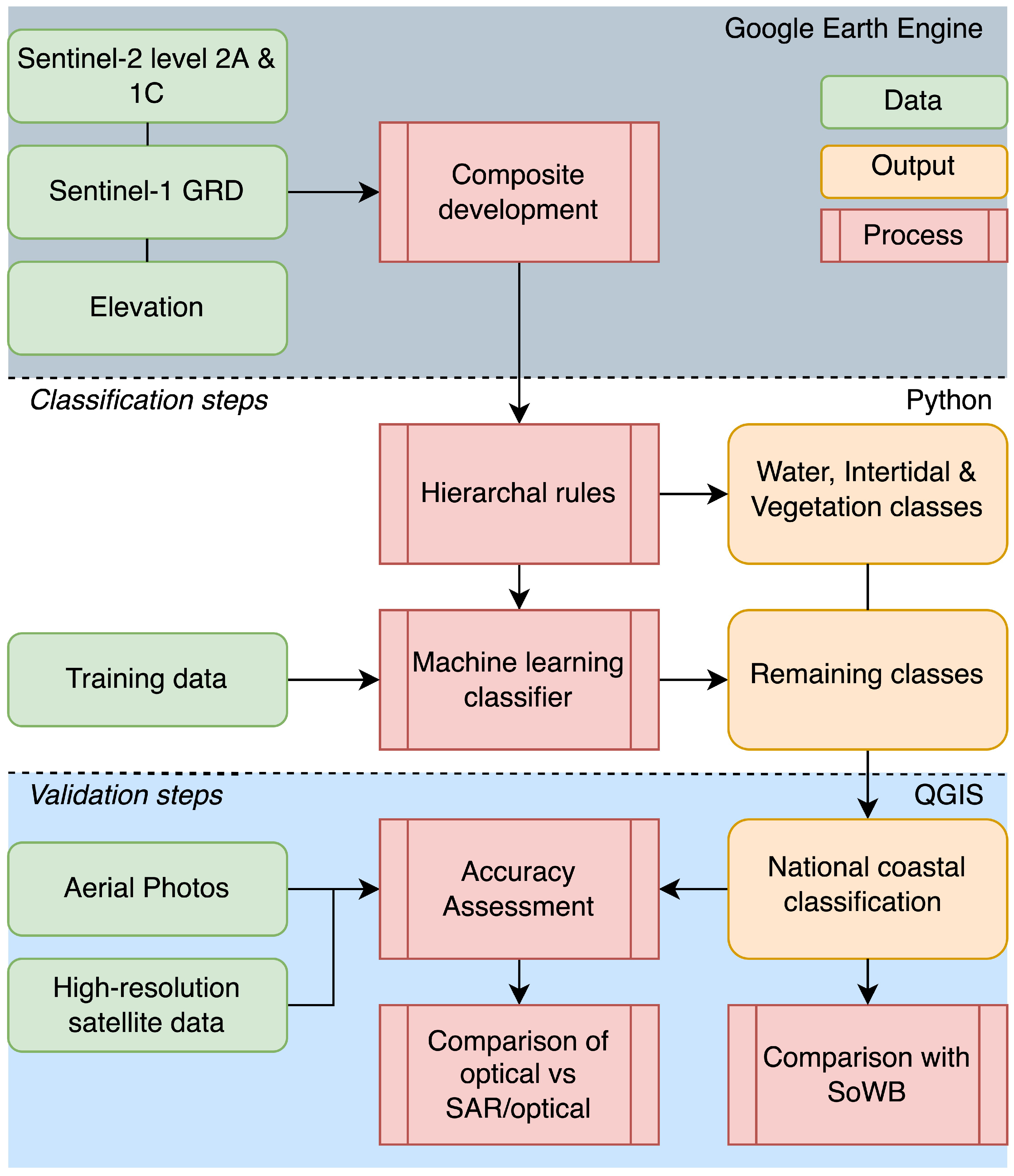
Figure 2. Summary of the classification workflow. Composite development was performed with Google Earth Engine, the classification and validation steps were performed with Python and QGIS software packages.
Remotesensing 14 04827 g002
Figure 3. For each image in the top-of-atmosphere collection normalised difference water index (NDWI), modified normalised difference water index (MNDWI), and automated water extraction index (AWEI) were calculated to derive the statistical aggregations to generate the composite bands. Each image in the surface reflectance collection was used to calculate normalised difference vegetation index (NDVI). Multispectral and NDVI composite bands were derived from the surface reflectance imagery.
Remotesensing 14 04827 g003
Figure 4. Example of the steps applied imagery to (a) Generate composite images. (b) Mask artificial surfaces. (c) Apply rules to separate land, water and intertidal areas. (d) Classify remaining pixels with supervised machine learning. (e) Merge all classes and regions to produce a national scale classification.
Remotesensing 14 04827 g004
Figure 5. Class hierarchy was determined by the rules that were used to separate spectrally distinct classes. Remaining classes were identified with random forest machine learning.
Remotesensing 14 04827 g005
Figure 6. Example from one of the 106 locations at Kaikoura where comparisons were made between: (a) Transects adapted from [24], which were assigned sandy or non-sandy by the supervised classification used in that study. (b) The corresponding set of points generated at each location to validate the classification.
Remotesensing 14 04827 g006
Figure 7. Classification outputs for (a) Piha (b) Tairua (c) Gisborne (d) Kaikoura compared against aerial photos from the same time instance (2019) indicating that the workflow is successful at detecting sedimentary landcover types at the New Zealand coast, but white-water associated with breaking waves on wave-dominated coast are incorrectly classified as intertidal.
Remotesensing 14 04827 g007
Figure 8. Comparison of (a) High-resolution aerial photo of Motueka Island near Nelson (2019). (b) Classification output for the same region. Intertidal areas were well identified in estuaries.
Remotesensing 14 04827 g008
Figure 9. F1-scores where Sentinel-2 and combination of Sentinel-1 and 2 data was used in the workflow. Accuracy of all sedimentary classes increased where SAR data was also used in the classification workflow.
Remotesensing 14 04827 g009
Figure 10. Box plots showing the distribution of clear observations for correctly and incorrectly classified pixels from the top-of-atmosphere and surface reflectance collections. Outliers were excluded as areas with high numbers of observations associated with tile overlap represent a small proportion of the overall area classified.
Remotesensing 14 04827 g010
Table 1. Summary of the statistical aggregations included in the composite imagery for both earth observation datasets used in the classification workflow.
DataComposite Bands
visible, NIR, SWIR15th percentile
NDVIInterval mean 10–90
NDWI, MNDWI, AWEIMinimum, Maximum, Median, Standard deviation, 10th percentile, 25th percentile, 50th percentile, 75th percentile, 90th percentile
SARVV ascending orbit, VH ascending orbit, VH:VV ascending orbit, VV descending orbit, VH descending orbit, VH:VV descending orbit
Table 2. Summary of class nomenclature.
ClassDescriptionAerial Photo
Artificial surfacesAny built surface or buildings associated with commercial, residential or industrial use including surrounding infrastructure, amenities and transport routes. Remotesensing 14 04827 i001
Bare rockBare surfaces dominated by unconsolidated or consolidated material that is coarser than coarse gravel.Remotesensing 14 04827 i002
Dark sandSurfaces containing high concentrations of heavy minerals such as plagioclase, augite and titanomagnetite material that is finer than coarse sand (2 mm) along the coast.Remotesensing 14 04827 i003
GravelSurfaces dominated by unconsolidated material that is finer than coarse gravel and larger than coarse sand (2–60 mm).Remotesensing 14 04827 i004
IntertidalStanding or flowing saline water that includes estuaries, lagoons and surfaces that are diurnally covered by water due to tidal inundation.Remotesensing 14 04827 i005
Light sandSurfaces predominantly constituted by quartz, feldspar, mafic minerals and residue (lithic and shell fragments) material that is finer than coarse sand (2 mm) along the coast.Remotesensing 14 04827 i006 
Supratidal sandSurfaces predominantly constituted by material finer than coarse sand (2 mm), above the high water mark, that can be very sparsely vegetated and texturally different due to aeolian processes.Remotesensing 14 04827 i007 
VegetationAny surface (managed or natural) that is dominated by vegetation of any species in the coastal zone.Remotesensing 14 04827 i008
WaterOffshore or inshore permanent saline or fresh open water in the coastal zone including artificial lakes or ponds.Remotesensing 14 04827 i009 
Table 3. Training samples were proportional to the area of each class in the national scale training dataset as using area-proportional training has led to better results for classification trees [70].
ClassTraining SamplesProportion (%)
Bare rock23471.9
Dark sand34372.78
Gravel12,2419.92
Intertidal48,54639.33
Light sand51,57341.78
Supratidal sand52984.29
Table 4. Summary of regional and national accuracy metrics.
RegionProportion CorrectAllocation DisagreementQuantity DisagreementOverall Accuracy
Auckland0.9710.0210.0080.935
Bay of Plenty0.9670.0090.0240.888
Canterbury0.9620.0050.0330.846
Gisborne0.9690.0040.0270.855
Hawkes Bays0.9580.0010.0410.828
Manawatu0.8280.0160.1570.84
Marlborough0.98700.0120.911
Nelson0.9910.0040.0060.911
Northland0.9750.0180.0070.869
Otago0.94500.0540.881
Southland0.8480.0050.1470.765
Taranaki0.86900.1310.876
Tasman0.9830.0040.0130.895
Waikato0.9720.0130.0150.91
Wellington0.8410.0010.1580.822
West Coast0.8790.0020.1190.833
National0.9360.0120.0530.864
Table 5. National producer and user accuracy for each class and commission/omission after normalising the confusion matrix by the area of each class.
ClassF1-ScoreUser Accuracy (%)Producer Accuracy (%)CommissionOmissionArea (Hectares)
Artificial surfaces0.9299.585.440.00040.001250,710,640
Bare rock0.993.7586.6100.0011471,904
Dark sand0.8593.794.4600.001191,296
Gravel0.8374.3593.290.00120.00063,401,184
Intertidal0.6954.4495.110.05370.002884,433,392
Light sand0.8575.9595.590.00330.0029,885,152
Supratidal sand0.9486.584.2700.0016436,336
Vegetation0.9499.9588.180.00010.001889,672,432
Water0.8199.1569.060.00570.0523474,867,472
Table 6. Comparison of national accuracy metrics where combination of Sentinel-1 and Sentinel-2 data were used in the classification workflow and only Sentinel-2 data was used.
DataProportion CorrectAllocation DisagreementQuantity DisagreementOverall Accuracy
Sentinel-1 and 20.9360.0120.0530.864
Sentinel-20.8990.0180.0830.721
Publisher’s Note: MDPI stays neutral with regard to jurisdictional claims in published maps and institutional affiliations.