
Cloud Contaminated Multispectral Remote Sensing Image Enhancement Algorithm Based on MobileNet

Abstract

1. Introduction
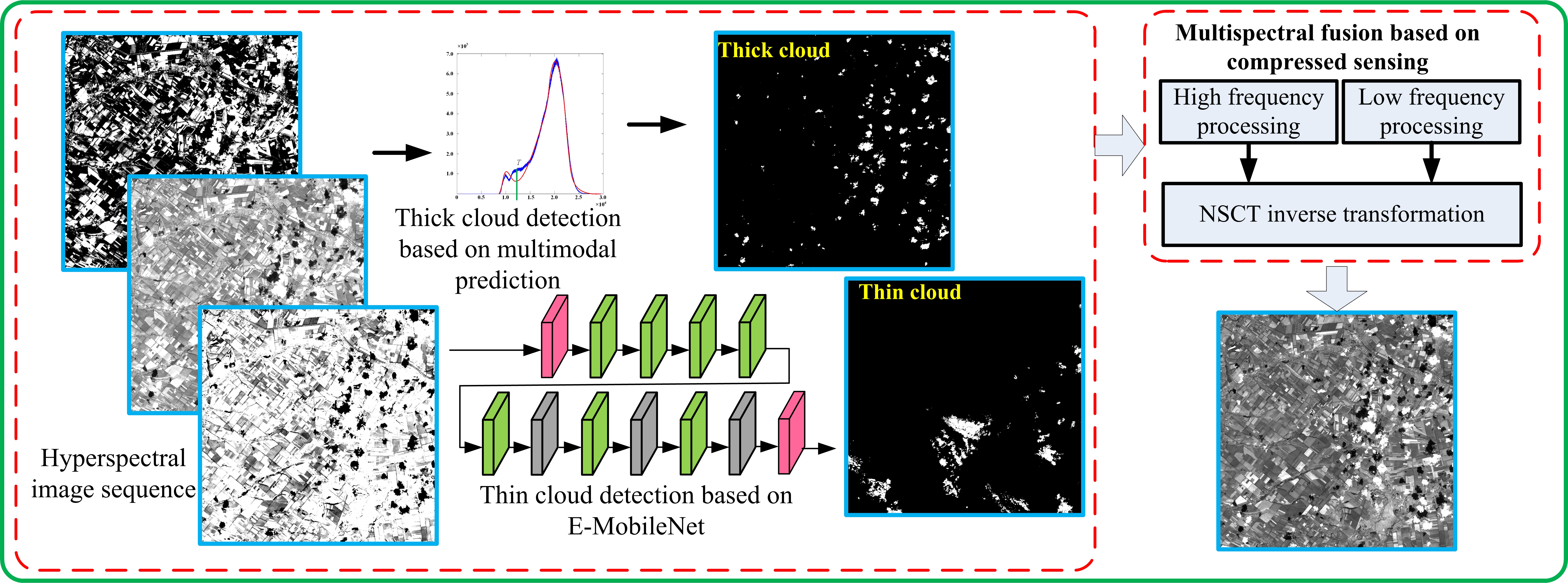
2. Methods
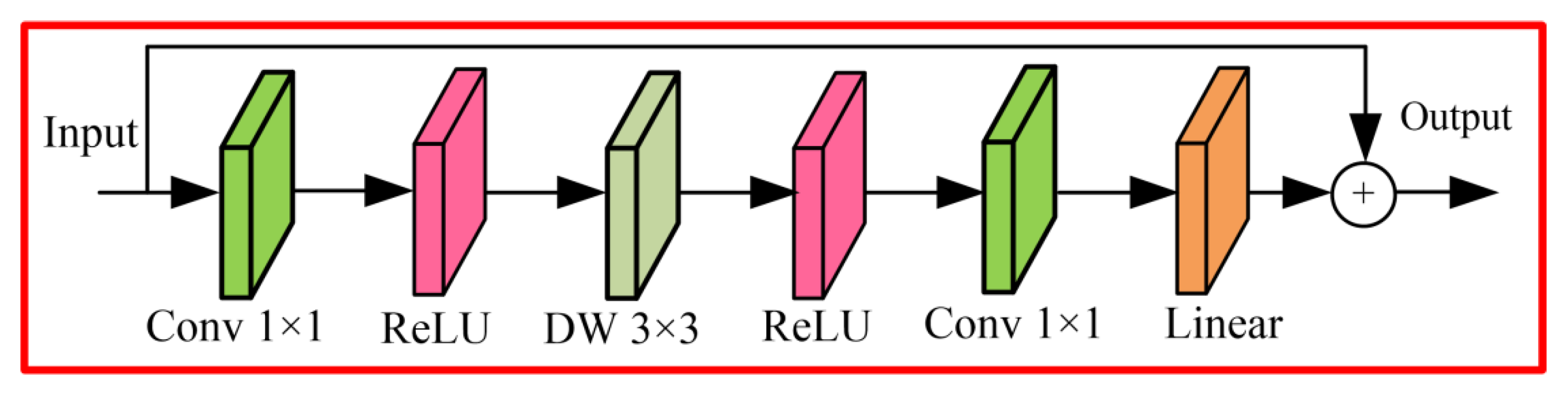
2.1. MobileNet
2.2. Cloud Detection Algorithm Based on Improved MobileNet
2.3. Self-Supervised Training Algorithm
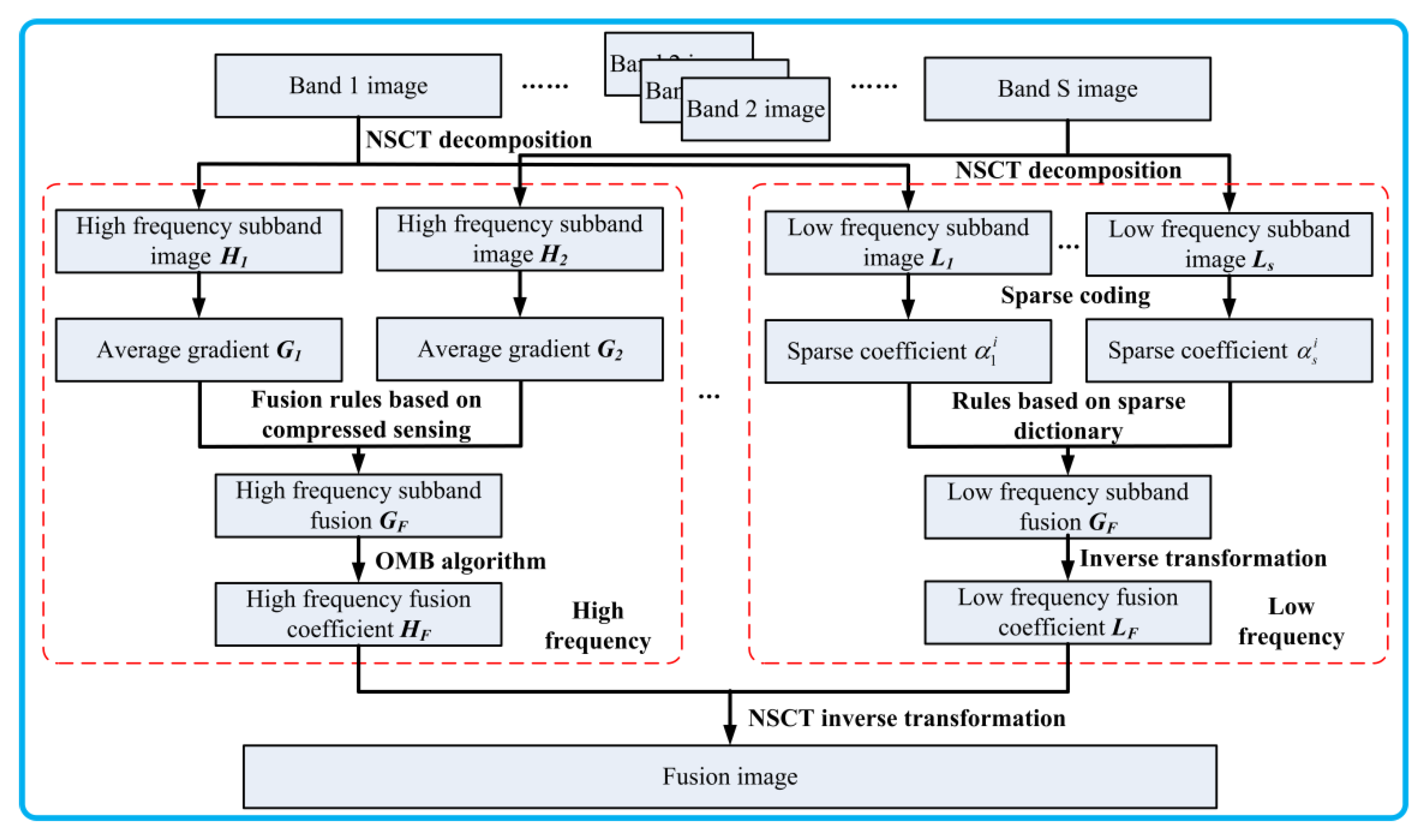
2.4. Multispectral Fusion Algorithm Based on Compressed Sensing
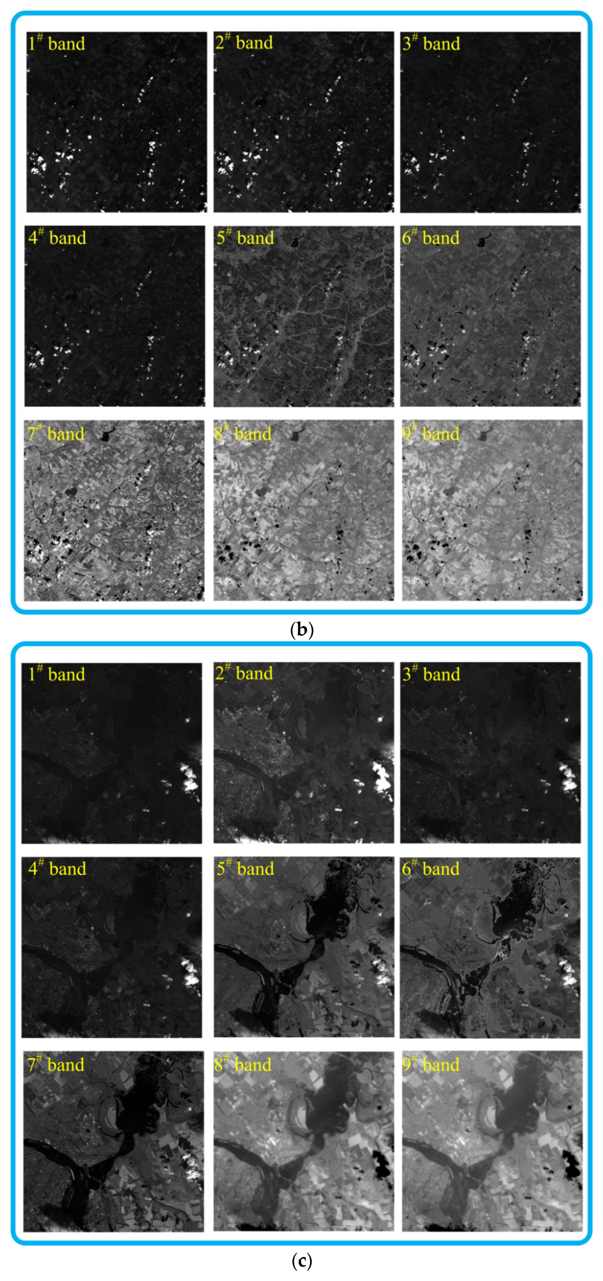
3. Dataset Description
4. Experiment Analysis
4.1. Performance of the Cloud Detection Algorithm
4.2. Performance of the Training Algorithm
4.3. Evaluation of Image Enhancement Effect
5. Conclusions
Author Contributions
Funding
Data Availability Statement
Acknowledgments
Conflicts of Interest
References
- Li, L.; Li, X.; Jiang, L.; Su, X.; Chen, F. A review on deep learning techniques for cloud detection methodologies and challenges. Signal. Image Video Process. 2021, 15, 1527–1535. [Google Scholar] [CrossRef]
- Poli, G.; Adembri, G.; Gherardelli, M.; Tommasini, M. Dynamic threshold cloud detection algorithm improvement for AVHRR and SEVIRI images. In Proceedings of the 2010 IEEE International Geoscience and Remote Sensing Symposium, Honolulu, HI, USA, 25–30 July 2010; pp. 4146–4149. [Google Scholar]
- Lin, C.-H.; Lin, B.-Y.; Lee, K.-Y.; Chen, Y.-C. Radiometric normalization and cloud detection of optical satellite images using invariant pixels. ISPRS J. Photogramm. Remote Sens. 2015, 106, 107–117. [Google Scholar] [CrossRef]
- Başeski, E.; Cenaras, Ç. Texture and color based cloud detection. In Proceedings of the 2015 7th international conference on recent advances in space technologies (RAST), Istanbul, Turkey, 16–19 June 2015; pp. 311–315. [Google Scholar]
- Addesso, P.; Conte, R.; Longo, M.; Restaino, R.; Vivone, G. MAP-MRF cloud detection based on PHD filtering. IEEE J. Sel. Top. Appl. Earth Obs. Remote Sens. 2012, 5, 919–929. [Google Scholar] [CrossRef]
- Surya, S.R.; Simon, P. Automatic cloud detection using spectral rationing and fuzzy clustering. In Proceedings of the 2013 2nd International Conference on Advanced Computing, Networking and Security, Mangalore, India, 15–17 December 2013; pp. 90–95. [Google Scholar]
- Zhang, Q.; Xiao, C. Cloud Detection of RGB Color Aerial Photographs by Progressive Refinement Scheme. IEEE Trans. Geosci. Remote Sens. 2014, 52, 7264–7275. [Google Scholar] [CrossRef]
- Zi, Y.; Xie, F.; Jiang, Z. A Cloud Detection Method for Landsat 8 Images Based on PCANet. Remote Sens. 2018, 10, 877. [Google Scholar] [CrossRef]
- He, W.; Zhang, H.; Shen, H.; Zhang, L. Hyperspectral Image Denoising Using Local Low-Rank Matrix Recovery and Global Spatial–Spectral Total Variation. IEEE J. Sel. Top. Appl. Earth Obs. Remote Sens. 2018, 11, 713–729. [Google Scholar] [CrossRef]
- Onsi, M.; ElSaban, H. Spatial cloud detection and retrieval system for satellite images. Int. J. Adv. Comput. Sci. Appl. 2012, 3, 12. [Google Scholar]
- Changhui, Y.; Yuan, Y.; Minjing, M.; Menglu, Z. Cloud detection method based on feature extraction in remote sensing images. Int. Arch. Photogramm. Remote Sens. Spat. Inf. Sci. 2013, 2, W1. [Google Scholar] [CrossRef]
- Xie, F.; Shi, M.; Shi, Z.; Yin, J.; Zhao, D. Multilevel cloud detection in remote sensing images based on deep learning. IEEE J. Sel. Top. Appl. Earth Obs. Remote Sens. 2017, 10, 3631–3640. [Google Scholar] [CrossRef]
- Shao, Z.; Deng, J.; Wang, L.; Fan, Y.; Sumari, N.S.; Cheng, Q. Fuzzy autoencode based cloud detection for remote sensing imagery. Remote Sens. 2017, 9, 311. [Google Scholar] [CrossRef]
- Chen, Y.; Guo, Y.; Wang, Y.; Wang, D.; Peng, C.; He, G. Denoising of hyperspectral images using nonconvex low rank matrix approximation. IEEE Trans. Geosci. Remote Sens. 2017, 55, 5366–5380. [Google Scholar] [CrossRef]
- Zhang, X.; Qin, F.; Qin, Y. Study on the thick cloud removal method based on multi-temporal remote sensing images. In Proceedings of the 2010 International Conference on Multimedia Technology, Ningbo, China, 29–31 October 2010; pp. 1–3. [Google Scholar]
- Marais, I.V.Z.; Du Preez, J.A.; Steyn, W.H. An optimal image transform for threshold-based cloud detection using heteroscedastic discriminant analysis. Int. J. Remote Sens. 2011, 32, 1713–1729. [Google Scholar] [CrossRef]
- Qian, J.; Luo, Y.; Wang, Y.; Li, D. Cloud detection of optical remote sensing image time series using mean shift algorithm. In Proceedings of the 2016 IEEE International Geoscience and Remote Sensing Symposium (IGARSS), Beijing, China, 10–15 July 2016; pp. 560–562. [Google Scholar]
- Wei, Q.; Bioucas-Dias, J.; Dobigeon, N.; Tourneret, J.Y. Hyperspectral and multispectral image fusion based on a sparse representation. IEEE Trans. Geosci. Remote Sens. 2015, 53, 3658–3668. [Google Scholar] [CrossRef]
- Hu, G.; Sun, X.; Liang, D.; Sun, Y. Cloud removal of remote sensing image based on multi-output support vector regression. J. Syst. Eng. Electron. 2014, 25, 1082–1088. [Google Scholar] [CrossRef]
- Sui, Y.; He, B.; Fu, T. Energy-based cloud detection in multispectral images based on the SVM technique. Int. J. Remote Sens. 2019, 40, 5530–5543. [Google Scholar] [CrossRef]
- Li, Y.; Chen, W.; Zhang, Y.; Tao, C.; Xiao, R.; Tan, Y. Accurate cloud detection in high-resolution remote sensing imagery by weakly supervised deep learning. Remote Sens. Environ. 2020, 250, 112045. [Google Scholar] [CrossRef]
- Villa, A.; Chanussot, J.; Benediktsson, J.A.; Jutten, C.; Dambreville, R. Unsupervised methods for the classification of hyperspectral images with low spatial resolution. Pattern Recognit. 2013, 46, 1556–1568. [Google Scholar] [CrossRef]
- Ozkan, S.; Efendioglu, M.; Demirpolat, C. Cloud detection from RGB color remote sensing images with deep pyramid networks. In Proceedings of the IGARSS 2018—2018 IEEE International Geoscience and Remote Sensing Symposium, Valencia, Spain, 22–27 July 2018; pp. 6939–6942. [Google Scholar]
- Liu, H.; Zeng, D.; Tian, Q. Super-pixel cloud detection using hierarchical fusion CNN. In Proceedings of the2018 IEEE Fourth International Conference on Multimedia Big Data (BigMM), Xi’an, China, 13–16 September 2018; pp. 1–6. [Google Scholar]
- He, Q.; Sun, X.; Yan, Z.; Fu, K. DABNet: Deformable contextual and boundary-weighted network for cloud detection in remote sensing images. IEEE Trans. Geosci. Remote Sens. 2021, 60, 29. [Google Scholar] [CrossRef]
- Yuan, Q.; Zhang, Q.; Li, J.; Shen, H.; Zhang, L. Hyperspectral image denoising employing a spatial–spectral deep residual convolutional neural network. IEEE Trans. Geosci. Remote Sens. 2019, 57, 1205–1218. [Google Scholar] [CrossRef]
- Bai, T.; Li, D.; Sun, K.; Chen, Y.; Li, W. Cloud detection for high-resolution satellite imagery using machine learning and multi-feature fusion. Remote Sens. 2016, 8, 715. [Google Scholar] [CrossRef]
- Zhang, J.; Li, X.; Li, L.; Sun, P.; Su, X.; Hu, T.; Chen, F. Lightweight U-Net for cloud detection of visible and thermal infrared remote sensing images. Opt. Quantum Electron. 2020, 52, 397. [Google Scholar] [CrossRef]
- Zhang, J.; Zhou, Q.; Shen, X.; Li, Y. Cloud detection in high-resolution remote sensing images using multi-features of ground objects. J. Geovisualization Spat. Anal. 2019, 3, 14. [Google Scholar] [CrossRef]
- Zhang, J.; Wang, Y.; Wang, H.; Wu, J.; Li, Y. CNN cloud detection algorithm based on channel and spatial attention and probabilistic upsampling for remote sensing image. IEEE Trans. Geosci. Remote Sens. 2021, 60, 1–13. [Google Scholar] [CrossRef]
- Wei, K.; Fu, Y.; Huang, H. 3-D quasi-recurrent neural network for hyperspectral image denoising. IEEE Trans. Neural Netw. Learn. Syst. 2021, 32, 363–375. [Google Scholar] [CrossRef]
- Hwang, S.J.; Kapoor, A.; Kang, S.B. Context-based automatic local image enhancement. In European Conference on Computer Vision; Springer: Berlin/Heidelberg, Germany, 2012; pp. 569–582. [Google Scholar]
- Bai, X.; Zhou, F.; Xue, B. Image enhancement using multi scale image features extracted by top-hat transform. Opt. Laser Technol. 2012, 44, 328–336. [Google Scholar] [CrossRef]
- Özay, E.K.; Tunga, B. A novel method for multispectral image pansharpening based on high dimensional model representation. Expert Syst. Appl. 2021, 170, 114512. [Google Scholar] [CrossRef]
- Choi, Y.; Kim, N.; Hwang, S.; Kweon, I.S. Thermal image enhancement using convolutional neural network. In Proceedings of the 2016 IEEE/RSJ international conference on intelligent robots and systems (IROS), Daejeon, Korea, 9–14 October 2016; pp. 223–230. [Google Scholar]
- Zhuang, P.; Li, C.; Wu, J. Bayesian retinex underwater image enhancement. Eng. Appl. Artif. Intell. 2021, 101, 104171. [Google Scholar] [CrossRef]
- Mehranian, A.; Wollenweber, S.D.; Walker, M.D.; Bradley, K.M.; Fielding, P.A.; Su, K.H.; McGowan, D.R. Image enhancement of whole-body oncology [18F]-FDG PET scans using deep neural networks to reduce noise. Eur. J. Nucl. Med. Mol. Imaging 2022, 49, 539–549. [Google Scholar] [CrossRef]
- Mahashwari, T.; Asthana, A. Image enhancement using fuzzy technique. Int. J. Res. Eng. Sci. Technol. 2013, 2, 1–4. [Google Scholar]
- Singh, K.; Kapoor, R. Image enhancement using exposure based sub image histogram equalization. Pattern Recognit. Lett. 2014, 36, 10–14. [Google Scholar] [CrossRef]
- Raju, G.; Nair, M.S. A fast and efficient color image enhancement method based on fuzzy-logic and histogram. AEU-Int. J. Electron. Commun. 2014, 68, 237–243. [Google Scholar] [CrossRef]
- Chen, S.; Liu, Y.; Zhang, C. Water-Body segmentation for multi-spectral remote sensing images by feature pyramid enhancement and pixel pair matching. Int. J. Remote Sens. 2021, 42, 5025–5043. [Google Scholar] [CrossRef]
- Liu, X.; Bourennane, S.; Fossati, C. Denoising of hyperspectral images using the PARAFAC model and statistical performance analysis. IEEE Trans. Geosci. Remote Sens. 2012, 50, 3717–3724. [Google Scholar] [CrossRef]
- Pathak, S.S.; Dahiwale, P.; Padole, G. A combined effect of local and global method for contrast image enhancement. In Proceedings of the 2015 IEEE International Conference on Engineering and Technology (ICETECH), Coimbatore, India, 20 March 2015; pp. 1–5. [Google Scholar]
- Goldstein, T.; Xu, L.; Kelly, K.F.; Baraniuk, R. The stone transform: Multi-resolution image enhancement and compressive video. IEEE Trans. Image Process. 2015, 24, 5581–5593. [Google Scholar] [CrossRef]
- Xu, Y.; Yang, C.; Sun, B.; Yan, X.; Chen, M. A novel multi-scale fusion framework for detail-preserving low-light image enhancement. Inf. Sci. 2021, 548, 378–397. [Google Scholar] [CrossRef]
- Stankevich, S.A.; Piestova, I.O.; Lubskyi, M.S.; Shklyar, S.V.; Lysenko, A.R.; Maslenko, O.V.; Rabcan, J. Knowledge-based multispectral remote sensing imagery superresolution. In Reliability Engineering and Computational Intelligence; Springer: Cham, Switzerland, 2021; pp. 219–236. [Google Scholar]
- Rahman, S.; Rahman, M.M.; Abdullah-Al-Wadud, M.; Al-Quaderi, G.D.; Shoyaib, M. An adaptive gamma correction for image enhancement. EURASIP J. Image Video Process. 2016, 1, 1–13. [Google Scholar] [CrossRef]
- Li, M.; Liu, J.; Yang, W.; Sun, X.; Guo, Z. Structure-revealing low-light image enhancement via robust retinex model. IEEE Trans. Image Process. 2018, 27, 2828–2841. [Google Scholar] [CrossRef]
- Kuang, X.; Sui, X.; Liu, Y.; Chen, Q.; Gu, G. Single infrared image enhancement using a deep convolutional neural network. Neurocomputing 2019, 332, 119–128. [Google Scholar] [CrossRef]
- Usharani, A.; Bhavana, D. Deep convolution neural network based approach for multispectral images. Int. J. Syst. Assur. Eng. Manag. 2021, 1–10. [Google Scholar] [CrossRef]
- Chen, Y.; He, W.; Yokoya, N.; Huang, T.Z.; Zhao, X.L. Nonlocal tensor-ring decomposition for hyperspectral image denoising. IEEE Trans. Geosci. Remote Sens. 2020, 58, 1348–1362. [Google Scholar] [CrossRef]
- Wen, H.; Tian, Y.; Huang, T.; Gao, W. Single underwater image enhancement with a new optical model. In Proceedings of the 2013 IEEE International Symposium on Circuits and Systems (ISCAS), Beijing, China, 19–23 May 2013; pp. 753–756. [Google Scholar]
- Shen, L.; Yue, Z.; Feng, F.; Chen, Q.; Liu, S.; Ma, J. Msr-net: Low-light image enhancement using deep convolutional network. arXiv 2017, arXiv:1711.02488. [Google Scholar]
- Kaplan, N.H. Remote sensing image enhancement using hazy image model. Optik 2018, 155, 139–148. [Google Scholar] [CrossRef]
- Liu, K.; Liang, Y. Underwater image enhancement method based on adaptive attenuation-curve prior. Opt. Express 2021, 29, 10321–10345. [Google Scholar] [CrossRef]
- Zhou, M.; Jin, K.; Wang, S.; Ye, J.; Qian, D. Color retinal image enhancement based on luminosity and contrast adjustment. IEEE Trans. Biomed. Eng. 2017, 65, 521–527. [Google Scholar] [CrossRef]
- Kim, H.U.; Koh, Y.J.; Kim, C.S. PieNet: Personalized image enhancement network. In European Conference on Computer Vision; Springer: Cham, Switzerland, 2020; pp. 374–390. [Google Scholar]
- Moran, S.; Marza, P.; McDonagh, S.; Parisot, S.; Slabaugh, G. Deeplpf: Deep local parametric filters for image enhancement. In Proceedings of the IEEE/CVF Conference on Computer Vision and Pattern Recognition, Seattle, WA, USA, 13–19 June 2020; pp. 12826–12835. [Google Scholar]
- Li, Y.; Huang, H.; Xie, Q.; Yao, L.; Chen, Q. Research on a surface defect detection algorithm based on MobileNet-SSD. Appl. Sci. 2018, 8, 1678. [Google Scholar] [CrossRef]
- Kadam, K.; Ahirrao, S.; Kotecha, K.; Sahu, S. Detection and localization of multiple image splicing using MobileNet V1. IEEE Access 2021, 9, 162499–162519. [Google Scholar] [CrossRef]
- Srinivasu, P.N.; SivaSai, J.G.; Ijaz, M.F.; Bhoi, A.K.; Kim, W.; Kang, J.J. Classification of skin disease using deep learning neural networks with MobileNet V2 and LSTM. Sensors 2021, 21, 2852. [Google Scholar] [CrossRef]
- Kavyashree, P.S.; El-Sharkawy, M. Compressed mobilenet v3: A light weight variant for resource-constrained platforms. In Proceedings of the 2021 IEEE 11th Annual Computing and Communication Workshop and Conference (CCWC), Online. 27–30 January 2021; pp. 104–107. [Google Scholar]
- Al-Rahlawee, A.T.H.; Rahebi, J. Multilevel thresholding of images with improved Otsu thresholding by black widow optimization algorithm. Multimed. Tools Appl. 2021, 80, 28217–28243. [Google Scholar] [CrossRef]
- Arif, M.; Wang, G. Fast curvelet transform through genetic algorithm for multimodal medical image fusion. Soft Comput. 2020, 24, 1815–1836. [Google Scholar] [CrossRef]
- Qiu, S.; Tang, Y.; Du, Y.; Yang, S. The infrared moving target extraction and fast video reconstruction algorithm. Infrared Phys. Technol. 2019, 97, 85–92. [Google Scholar] [CrossRef]
- Srivastava, S.; Kumar, P.; Chaudhry, V.; Singh, A. Detection of ovarian cyst in ultrasound images using fine-tuned VGG-16 deep learning network. SN Comput. Sci. 2020, 1, 81. [Google Scholar] [CrossRef]
- Sam, S.M.; Kamardin, K.; Sjarif, N.N.A.; Mohamed, N. Offline signature verification using deep learning convolutional neural network (CNN) architectures GoogLeNet inception-v1 and inception-v3. Procedia Comput. Sci. 2019, 161, 475–483. [Google Scholar]
- Lu, Z.; Bai, Y.; Chen, Y.; Su, C.; Lu, S.; Zhan, T.; Wang, S. The classification of gliomas based on a pyramid dilated convolution resnet model. Pattern Recognit. Lett. 2020, 133, 173–179. [Google Scholar] [CrossRef]
- Vanmali, A.V.; Gadre, V.M. Visible and NIR image fusion using weight-map-guided Laplacian–Gaussian pyramid for improving scene visibility. Sādhanā 2017, 42, 1063–1082. [Google Scholar] [CrossRef]


| Algorithm | Cloudy | Urban | Suburban | Average |
|---|---|---|---|---|
| Time (s) | 298 | 578 | 412 | 429 |
| Algorithm | AOM | AVM | AUM | CM |
|---|---|---|---|---|
| CTF [4] | 0.65 | 0.33 | 0.35 | 0.66 |
| MS [12] | 0.71 | 0.31 | 0.34 | 0.69 |
| SVM [20] | 0.75 | 0.26 | 0.27 | 0.74 |
| ACNN [30] | 0.76 | 0.21 | 0.25 | 0.77 |
| The proposed algorithm | 0.81 | 0.18 | 0.23 | 0.80 |
| Algorithm | AOM | AVM | AUM | CM |
|---|---|---|---|---|
| CTF [4] | 0.72 | 0.35 | 0.35 | 0.67 |
| MS [12] | 0.78 | 0.30 | 0.31 | 0.72 |
| SVM [20] | 0.80 | 0.26 | 0.22 | 0.77 |
| ACNN [30] | 0.82 | 0.17 | 0.19 | 0.82 |
| The proposed algorithm | 0.86 | 0.14 | 0.15 | 0.86 |
| Algorithm | AOM | AVM | AUM | CM |
|---|---|---|---|---|
| CTF [4] | 0.61 | 0.38 | 0.39 | 0.61 |
| MS [12] | 0.68 | 0.34 | 0.35 | 0.66 |
| SVM [20] | 0.76 | 0.26 | 0.31 | 0.73 |
| ACNN [30] | 0.80 | 0.21 | 0.23 | 0.79 |
| The proposed algorithm | 0.83 | 0.16 | 0.19 | 0.82 |
| Algorithm | AG | SD | SF | EI |
|---|---|---|---|---|
| LCM [56] | 9.2 | 46.2 | 33.5 | 5.1 |
| LEM [33] | 9.5 | 47.5 | 34.5 | 5.3 |
| SIH [39] | 9.8 | 46.9 | 35.8 | 6.2 |
| LGP [69] | 10.5 | 49.8 | 35.4 | 6.4 |
| CNN [30] | 10.3 | 52.8 | 36.8 | 6.5 |
| CVT [64] | 10.9 | 51.3 | 37.2 | 6.8 |
| MSF [45] | 11.2 | 52.6 | 36.5 | 7.1 |
| The proposed algorithm | 12.3 | 56.1 | 38.6 | 7.3 |
Publisher’s Note: MDPI stays neutral with regard to jurisdictional claims in published maps and institutional affiliations. |
© 2022 by the authors. Licensee MDPI, Basel, Switzerland. This article is an open access article distributed under the terms and conditions of the Creative Commons Attribution (CC BY) license (https://creativecommons.org/licenses/by/4.0/).
Share and Cite
Li, X.; Ye, H.; Qiu, S. Cloud Contaminated Multispectral Remote Sensing Image Enhancement Algorithm Based on MobileNet. Remote Sens. 2022, 14, 4815. https://doi.org/10.3390/rs14194815
Li X, Ye H, Qiu S. Cloud Contaminated Multispectral Remote Sensing Image Enhancement Algorithm Based on MobileNet. Remote Sensing. 2022; 14(19):4815. https://doi.org/10.3390/rs14194815
Chicago/Turabian StyleLi, Xuemei, Huping Ye, and Shi Qiu. 2022. "Cloud Contaminated Multispectral Remote Sensing Image Enhancement Algorithm Based on MobileNet" Remote Sensing 14, no. 19: 4815. https://doi.org/10.3390/rs14194815
APA StyleLi, X., Ye, H., & Qiu, S. (2022). Cloud Contaminated Multispectral Remote Sensing Image Enhancement Algorithm Based on MobileNet. Remote Sensing, 14(19), 4815. https://doi.org/10.3390/rs14194815