Learned Design of a Compressive Hyperspectral Imager for Remote Sensing by a Physics-Constrained Autoencoder

Abstract

Designing and optimizing systems by end-to-end deep learning is a recently emerging field. We present a novel physics-constrained autoencoder (PyCAE) for the design and optimization of a physically realizable sensing model. As a case study, we design a compressive hyperspectral imaging system for remote sensing based on this approach, which allows capturing hundreds of spectral bands with as few as four compressed measurements. We demonstrate our deep learning approach to design spectral compression with a spectral light modulator (SpLM) encoder and a reconstruction neural network decoder. The SpLM consists of a set of modified Fabry–Pérot resonator (mFPR) etalons that are designed to have a staircase-shaped geometry. Each stair occupies a few pixel columns of a push-broom-like spectral imager. The mFPR’s stairs can sample the earth terrain in along-track scanning from an airborne or spaceborne moving platform. The SpLM is jointly designed with an autoencoder by a data-driven approach, while spectra from remote sensing databases are used to train the system. The SpLM’s parameters are optimized by integrating its physically realizable sensing model in the encoder part of the PyCAE. The decoder part of the PyCAE implements the spectral reconstruction.

1. Introduction

In recent years, deep learning has been playing a major role in the field of hyperspectral imaging (HSI) [1,2,3,4,5,6,7,8,9,10,11]. Various deep neural networks (DNNs) have been proposed to classify spectra features and segmentation [3,5] and use band selection for better classification [10,11]. Recently, DNNs have been used for the reconstruction of high-dimensional spectra from a few bands of the spectrum. These spectra are acquired by compressive sensing HSI (CS HSI) techniques, which reduce the storage capacity occupied by the huge HS cubes [4,6,7] and reduce the effort associated with their acquisition.

Over the last decades, spectral imaging [12,13,14,15] has become progressively utilized in airborne and spaceborne remote sensing tasks [16,17], among many others. Today, it is used in many fields, such as vegetation science [18], urban mapping [19], geology [20], mineralogy [21], mine detection [22], and more. Most such spectral imagers take advantage of the platform’s motion and may acquire the spectral data from the visible to the infrared wavelength ranges, by performing along-track spatial scanning of the imaged object [14,23]. The spectral information can then be measured directly, that is, by first splitting it into spectral components using dispersive or diffractive optical elements, followed by direct measurement of each component. Another approach is to acquire the spectral information indirectly, incorporating multiplexed and coded spectral measurements. This allows the benefit from Fellgett’s multiplex advantage [24,25] and, therefore, provides a significant gain in optical throughput, at the cost of less intuitive system design and the need for post-processing. A well-known example of indirect spectral acquisition is Fourier transform spectroscopy, which is used both for spectrometry [26] and spectral imaging [27,28]. As conventional Fourier transform spectroscopy systems are based on mechanically scanned Michelson of Mach–Zehnder interferometers, they demand strict stability and precision requirements. Thus, in harsh aerial and space environments, significant sophistication in their mechanical construction is required, and high-cost translational stages are incorporated to preserve the interferometric stability [29,30]. The indirect spectral acquisition can also be achieved by utilizing voltage-driven liquid crystal phase retarders [31,32,33,34,35,36], evading the need for incorporating moving parts, which results in these strict stability requirements. One such system is the compressive sensing miniature ultra-spectral imaging (CS-MUSI) system presented in [32,33,35]. It performs spectral multiplexing by applying a variable voltage to a thick liquid crystal cell (LCC), thus achieving distinctive wideband spectral encodings.

Our group took the idea of CS-MUSI a step further to the remote sensing area by introducing a design that can be used with push-broom type scanning. In [37], we presented a wedge-shaped LCC that exploits a satellite’s motion along an orbit. Pixels of columns of the sensor behind the LCC capture the cross-track strips of the ground, each with a specific spectral modulation according to the height of the nematic liquid in front of the columns. The height of the nematic liquid changes linearly with the columns due to the geometric shape of the wedge (Figure 1b). Unlike CS-MUSI, wedge-shaped LCC passively changes the modulation of the light according to its geometrical shape; therefore, there is no need to apply different voltages to generate spectral modulations. Among the distinct properties of the wedge-shaped LCC-based spectral imager in [37] are its outstanding optical throughput (about two orders of magnitude higher than conventional HSI) and the ability to switch to panchromatic imaging mode.

With the wedge-shaped LCC (Figure 1b), the different modulations obtained by the continuously changed nematic liquid depth in front of various sensor’s columns determine the spectral linear sensing process that produces the spectral cube according to Equation (1).

$$g=\mathsf{\Phi }f,$$

(1)

where $g\in {ℝ}^{N_c}$ is the compressed spectrum, $N_c$ is the number of measurements, $\mathsf{\Phi }\in {ℝ}^{N_c\times N_{\lambda }}$ is the spectral sensing matrix, $N_{\lambda }$ is the number of spectral bands in the incoming signal, and $f\in {ℝ}^{N_{\lambda }}$ is the observed spectrum. On the other hand, the wedge-shaped LCC spectral modulation has a huge disadvantage, because the captured spectrum measurements are redundant, and thus, its acquired HS cube requires large memory storage and huge bandwidth capacity.

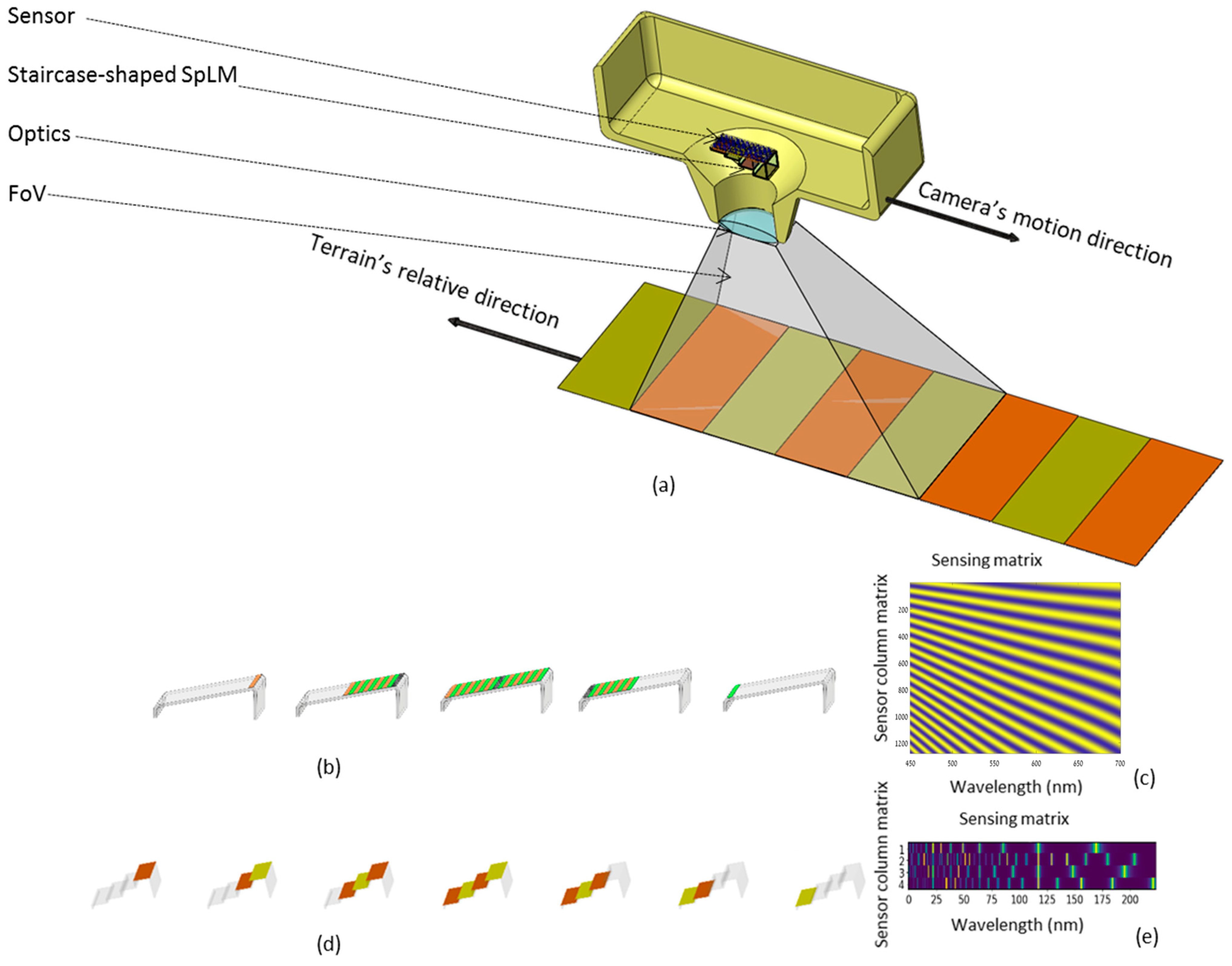
Figure 1a depicts the acquisition of the HS cube from the satellite. It describes the scanning along-track of an airborne or a spaceborne moving platform (in this case, a satellite camera equipped with an SpLM holding a staircase set of mFPR etalons [38]) scanning the earth terrain with a field of view (FoV) consisting of a sequence of the cross-track slices from the various stairs of the SpLM. The imager’s optics projects the scene on the mFPR etalons, and each etalon is placed in front of a sensor column, thus capturing the spectrally encoded spectrum of a cross-track strip on the ground. The stair may occupy multiple sensor columns so that upon appropriate processing (e.g., registration and averaging) it improves the robustness of the measurements. Figure 1b,d illustrates the difference between scanning the earth terrain with a wedge-shaped LCC and scanning the earth terrain with a staircase-shaped SpLM. In Figure 1b a continuous slant of the wedge-shaped LCC in front of the sensor’s columns dictates that each column should participate in the sampling with its own modulation and the resulting sensing matrix is overcomplete (e.g., taking 1250 measurements for 224 spectral bands).

In this paper, we keep evolving from the wedge-shaped LCC concept (based on CS-MUSI) [32,35], by using a set of mFPR etalons for SpLM (Figure 1d). In the staircase design, the width of the stairs is equal among all the stairs, so the image can be acquired continuously with the motion of the satellite in its orbit. The staircase design yields a novel CS HSI that:

(1)

Compresses the spectral information of the scene from $N_{\lambda }$ spectral bands to $N_s$ measurements respective to $N_s$ stairs in the SpLM,

(2)

Considers mFPR technology for the SpLM, which is applicable in a much broader spectral regime than the wedge-shaped LCC. Thus, instead of the wedge-shaped LCC (Figure 1b), here, we use a staircase-shaped set of mFPR etalons (see Figure 1d). The advantage of mFPR is that it can be used for a wider spectral range, including visible light and the SWIR ($0.4 \mathsf{\mu }\mathrm{m}–2.5 \mathsf{\mu }\mathrm{m}$).

The staircase shape of the SpLM allows it to sample the terrain with an undercomplete spectral sensing matrix; that is, to compress the signal to a few measurements only, while each stair occupies a few pixel columns. In this way, each measurement can be averaged from a few pixels in its corresponding row for the robustness of the measurement. Together, they determine the compressive spectral sensing matrix for each row $x$ under each stair $y$, which is used to compress the input signal. Similar to Equation (1), the sensing model is now described by Equation (2):

$$g_{cs}={\mathsf{\Phi }}_{cs}f,$$

(2)

where $g_{cs}\in {ℝ}^{N_s}$ is the compressed spectrum, $N_s$ is the number of stairs (measurements), and ${\mathsf{\Phi }}_{cs}\in {ℝ}^{N_s\times N_{\lambda }}$ is the compressive spectral sensing matrix.

In this paper, the optimal set of stairs height is learned by the PyCAE in an end-to-end fashion, from samples of remote-sensing HS cubes (i.e., Pavia center and Salinas valley [39]). A detailed description of the PyCAE will be given in the next section. After optimizing the height of the stairs, the encoder of the PyCAE can be replaced by a staircase-shaped set of mFPRs, and measurements from this SpLM are reconstructed by the PyCAE decoder.

Our contribution is as follows:

• We introduce a novel approach for learning the design and optimization of physical parameters of a system, by using a physics-constrained autoencoder (PyCAE).
• We introduce a new concept of a compressive sensing hyperspectral imager for remote sensing with high throughput and an extremely high compressive ratio of the spectral dimension.

2. Materials and Methods

2.1. Physics-Constrained Autoencoder (PyCAE)

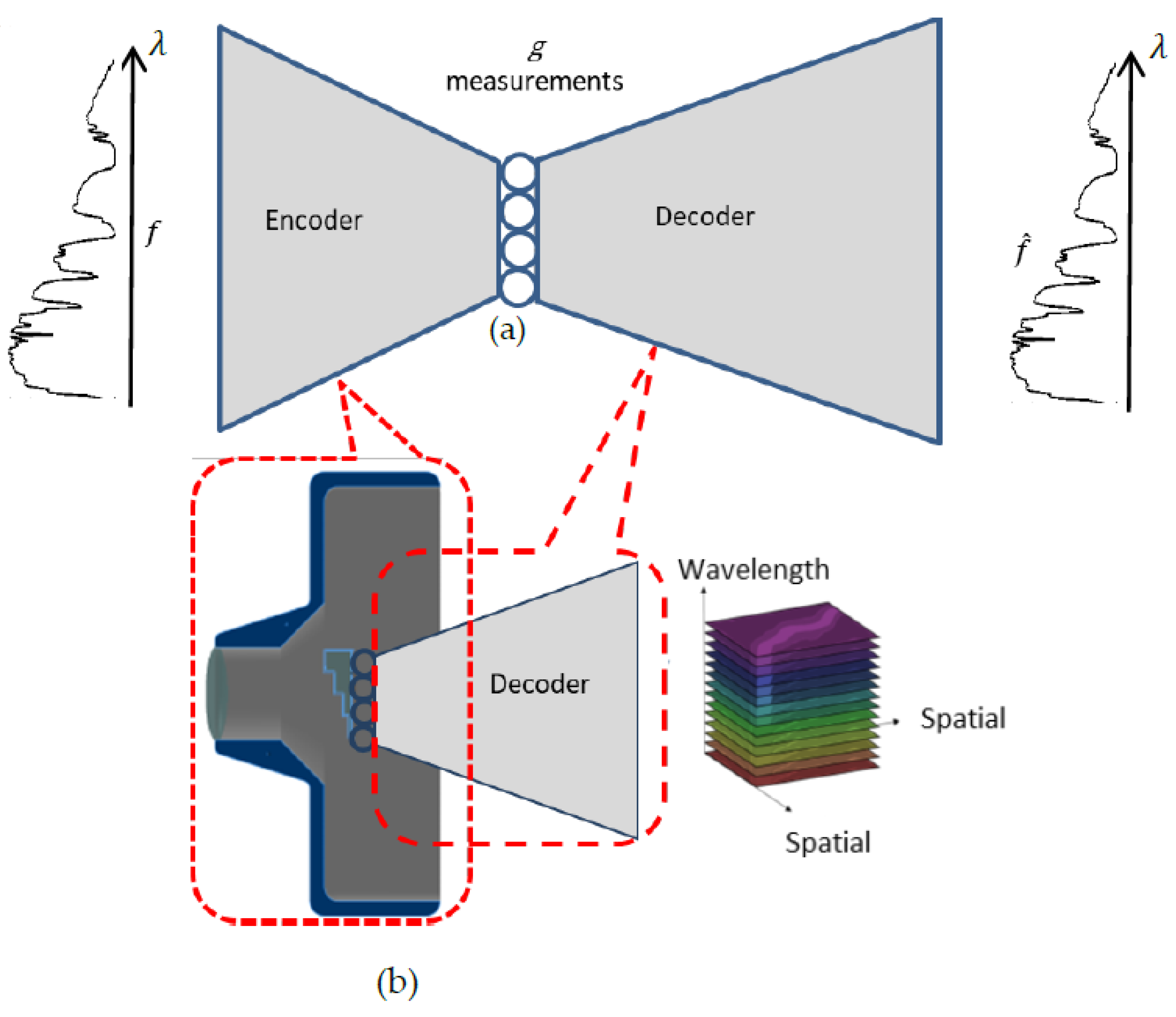
The proposed system consists of an encoder that emulates hardware with relay optics that images the light from the scene through the SpLM onto the sensor and software, which is a reconstruction DNN. The hardware can be modeled as a “sensing layer” and serves as the encoder of the PyCAE, while the reconstruction DNN serves as a decoder (Figure 2). The coupling between them holds the compressed measurements while serving as the bottleneck of the autoencoder. Unlike encoders of conventional deep learning autoencoders, in our model, the encoder is constrained to comply with the physics of our optical sensing hardware. Figure 2 depicts the general scheme of the system, including the deep learning model and respective sensing and reconstruction system.

PyCAE jointly optimizes the physical parameters that determine the values of the sensing matrix with the weights of the reconstruction DNN. Through its training process, we solve the following optimization problem:

$$\left\{\widehat{\theta },\widehat{W}\right\}=\underset{\theta ,W}{\mathrm{argmin}}{\mathbb{E}}_fℒ\left({\mathcal{N}}_{\theta ,W}\left(f\right),f\right)\hspace{1em}\hspace{1em}s.t. \in S_p$$

(3)

where ${\mathcal{N}}_{\theta ,W}=D_W\circ E_{\theta }$ is the PyCAE DNN consisting of the encoder $E_{\theta }$, which models the sensing matrix ${\mathsf{\Phi }}_{\theta }$, which depends on the physical parameters $\theta$, and of the decoder DNN $D_W$ with the trained weights W. $ℒ$ denotes the loss function (Section 2.6), and ${\mathbb{E}}_f$ denotes the expectation operator, practically evaluated as an average over the training set of spectra $f$. $S_p$ denotes a constrained set, in our case, dictated by the physics of the spectral modulation (see Section 2.2).

After training the autoencoder, the encoder “sensing layer” is detached from the decoder and replaced by the real physical device, which feeds its measurements into the reconstruction DNN, $D_W\left(g\right)$, where $g$ holds the measurements in the bottleneck of the PyCAE. In our case, the sensing layer is mathematically modeled by ${\mathsf{\Phi }}_{cs}$, which represents the transmission of the SpLM, depending on the parameters of the mFPR (see Section 2.2).

For training purposes, we feed a high-dimensional spectrum $f\in {ℝ}^{N_{\lambda }}$ with $N_{\lambda }$ spectral dimensions as an input of the encoder and feed the same spectrum to the autoencoder’s output, while the bottleneck holds $N_s\ll N_{\lambda }$ compressed measurements, $g\in {ℝ}^{N_s}$.

2.2. The SpLM and Its Model

In [38], we introduced the modified Fabry–Pérot Resonator (mFPR) for compressive hyperspectral imaging [36]. To obtain different spectral modulations for different measurements, refs. [38,40] modified the classical etalons in two fundamental ways. First, a wide range of gaps between the mirrors of the etalons is used to obtain more than a single spectral transmission peak, as in the case of classical FP-etalon. Second, the reflectivity of the mirrors is reduced by about $20\%-30\%$ to obtain multiple and wider spectral peaks. The array of the stairs set of the staircase-shaped mFPR is particularly adequate for this task, because it has good modulation, high throughput, and supports the visible and SWIR spectrum.

Here, we implement these etalons in the shape of stairs, so they can be used for compressive scanning imaging in the vertical direction of the stairs. We also model a BK7 glass as a substance to fill the etalons gaps, because it has good transparency to all the spectrum ranges we work on.

The spectral transmission of an ideal FP resonator is given by Equations (4) and (5) [38,40]:

$$T\left(\lambda \right)=\frac{1}{1+Fsi{n}^2\left(\raisebox{1ex}{$\delta \left(\lambda \right)$}\!\left/ \!\raisebox{-1ex}{$2$}\right.\right)},$$

(4)

where $\delta$ is the optical thickness, and $F$ is the finesse coefficients that are equal to

$$\delta \left(\lambda \right)=\frac{2\pi }{\lambda }2nd cos\left(\alpha \right); F=\frac{4R}{{\left(1-R\right)}^2}$$

(5)

where $\lambda$ is the wavelength, $n$ is the refractive index of the material between the two FP mirrors, and $\alpha$ is the incident angle of light. $R$ is the reflectivity of both mirrors that defines the full width at half-maximum (FWHM) of the spectral peaks. $d$ is the gap between the mirrors, which is responsible for the spectral modulation shape. As the gap grows, the number of the orders grows as well (i.e., the number of the spectral peaks). The gaps between the mirrors $d$ are the parameters that need to be optimized by the PyCAE to give a series of optimized modulations to construct an efficient sensing matrix. The spectral transmission $T\left(\lambda \right)$ is then the modulation of each stair of the SpLM, which is one line of the spectral sensing matrix ${\mathsf{\Phi }}_{\theta }$.

2.3. Encoder—Sensing Layer

Central to the PyCAE is the encoder, which models the sensing layer and reflects the spectral sensing matrix ${\mathsf{\Phi }}_{\theta }$. It represents a set of mFPR etalons forming the staircase shape (Figure 1d). Each stair in the staircase is an mFPR etalon whose height determines the gap ${\left\{d_i\right\}}_{i=1}^{N_s}$ between the mirrors of the etalon. By establishing each etalon’s gap $d$, the respective modulation of the spectral transmittance $T\left(\lambda \right)$ (given by Equation (4)) determines a row of the sensing matrix ${\mathsf{\Phi }}_{\theta }$. The bottleneck of the PyCAE, $g$, is the output of the encoder, and it holds the measurements according to Equation (6):

$$g_i={\displaystyle \sum }_{j\in \lambda }{T}_{ij}{f}_j,i=1,\cdots ,N_s,$$

(6)

where $T_{ij}$ is the $j^{th}$ wavelength transmittance of the mFPR at the $i^{th}$ stair (i.e., $T_{ij}=T\left({\lambda }_j;d_i\right)$), and $f_j$ is the intensity of the $j^{th}$ element of the spectrum of the incident light.

The encoder is used to optimize the SpLM’s parameters $\theta$ (e.g., the height of the stair-shaped mFPR’s etalons, ${\left\{d_i\right\}}_{i=1}^{N_s}$). It implements the physical model (Equation (4)) as its activation function, while the layer’s weights which reflect the height of the stairs are optimized parameters that are improved together with the reconstruction network’s weights at each iteration.

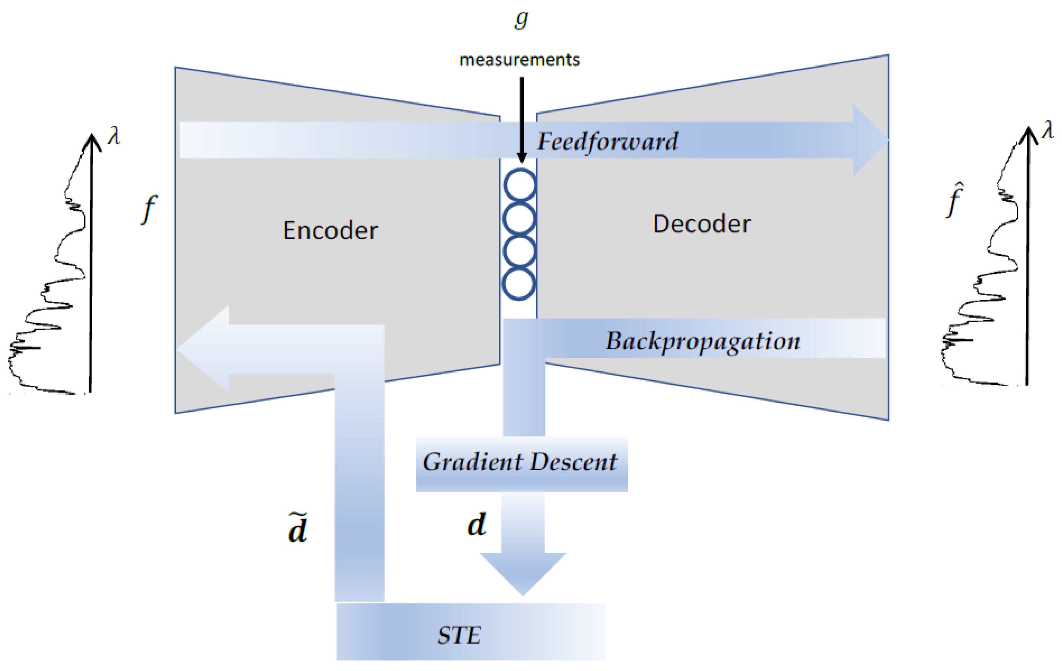
The optimized PyCAE’s encoder reflects the SpLM’s set of mFPR etalons (Figure 2); hence, the optimization process must consider the stairs’ physical constraints and the production limitations. To do so, we use the straight-through estimator (STE) technique, which was originally proposed by [41] for binary neural networks.

2.4. Straight-Through Estimator (STE)

To constrain the weights that represent the height of the stairs of the SpLM that are parametrized in the encoder, such as to be in a certain range of height and to have a minimum step of height between consecutive stairs, we use the STE algorithm.

According to the STE, at the feedforward phase, the input of the layer flows through the layer’s weights to the activation function of the layer, as if it had been the identity function [42]. But in the backpropagation phase, the flow of the gradients does not directly update the weights that represent the stairs’ heights ${\left\{d_i\right\}}_{i=1}^{N_s}$. Instead, the gradients update the weights according to Equations (7)–(9):

$$0.1 \mathsf{\mu }\mathrm{m}\ge {\theta }_i\ge 10 \mathsf{\mu }\mathrm{m},$$

(7)

$${\theta }_i=\{\begin{array}{cc}\frac{\lfloor {\theta }_i·10\rfloor }{10}+0.05,\hfill & \frac{\lfloor {\theta }_i·10\rfloor }{10}+0.05<{\theta }_i<\frac{\lfloor {\theta }_i·10\rfloor }{10}+0.1\\ \frac{\lfloor {\theta }_i·10\rfloor }{10},\hfill & \frac{\lfloor {\theta }_i·10\rfloor }{10}<{\theta }_i\le \frac{\lfloor {\theta }_i·10\rfloor }{10}+0.05\end{array}$$

(8)

$${\theta }_i≔{\theta }_i-\eta \mathsf{\Delta }L\left({\theta }_i\right),i=1,\cdots ,N_s$$

(9)

Equation (7) determines the range of depths for all the mFPR stairs between $0.1 \mathsf{\mu }\mathrm{m}$ and $10 \mathsf{\mu }\mathrm{m}$, and Equation (8) constrains the smallest step between consecutive stairs to be $50 \mathrm{nm}$. In Equation (9), ${\theta }_i$ of the encoder is the $i^{th}$ weight, which represents a gap $d_i$ of the $i^{th}$ mFPR etalon to be updated; $\eta$ is the learning rate; and $\partial L\left({\theta }_i\right)$ is the gradient, which backpropagates through the set of constraint functions as if it had been the identity of the activation function $T\left(d\right)$ (the function that represents the action of the mFPR etalons with respect to $d_i$). $\partial L\left(\theta \right)$ is calculated by the chain rule from the loss function at the output of the decoder, as shown in Equation (10):

$$\frac{\partial L\left(\theta \right)}{\partial \theta }=\frac{\partial L}{\partial w_n}·\frac{\partial w_n}{\partial a_{n-1}}\cdots \frac{\partial a_i}{\partial w_i}·\frac{\partial w_i}{\partial a_{i-1}}\cdots \frac{\partial a_1}{\partial w_1}·\frac{\partial w_1}{\partial T\left(\theta \right)}·\frac{\partial T\left(\theta \right)}{\partial \theta },$$

(10)

where $n$ is the number of layers in the decoder, $w_i$ are the weights of the $i^{th}$ layer of the decoder, and $a_i$ is the activation of the $i^{th}$ layer of the decoder.

Equation (11) shows the gradient of the mFPR etalons transmittance (Equations (4) and (5)) with respect to the depth $d_i$ of the etalons for an incident angle of light $\alpha =0^{°}$:

$$\frac{\partial L\left(\theta \right)}{\partial \theta }\equiv \frac{\partial T\left(d\right)}{\partial d}=\frac{-4\pi nFsin\left(\frac{2\pi n}{\lambda }d\right)\cos \left(\frac{2\pi n}{\lambda }d\right)}{\lambda {\left(1+Fsi{n}^2\left(\frac{2\pi n}{\lambda }d\right)\right)}^2},$$

(11)

Figure 3 and Algorithm 1 depict the STE mechanism:

Algorithm 1. Straight-Through Estimator (STE)

Initialization: Initialize weights due to model design constraints. (e.g., all weights value are between the minimum and maximum boundaries) Feedforward: Use current weights to flow information straight through the physical formula of the model. Backpropagation: Update weights by gradients flow through all layers from the output layer to the input layer (sensing layer). Deploy constraints on the updated weights to fit model requirements. (e.g., clip values between minimum and maximum boundaries).

In the case of a set of mFPR stairs of our SpLM, we constrain the range of the stair heights in the range of $0.1 \mathsf{\mu }\mathrm{m}–10 \mathsf{\mu }\mathrm{m}$ by clipping the weights in each iteration and limiting the minimum step between two stairs to $50 \mathrm{nm}$, by binning the weights in bins of $50 \mathrm{nm}$.

2.5. Decoder—Reconstruction DNN

The decoder of PyCAE serves as a reconstruction DNN. We designed it as a residual DNN following the general scheme of the DR2-net [43]. DR2-net was developed initially to reconstruct 2D images from compressed images; therefore, we adapted it to accept 1-dimensional (1D) spectra, as we successfully did in [6]. We modified the kernel sizes for each layer in a residual block (as they are hyperparameters of the network) to a 1D kernel.

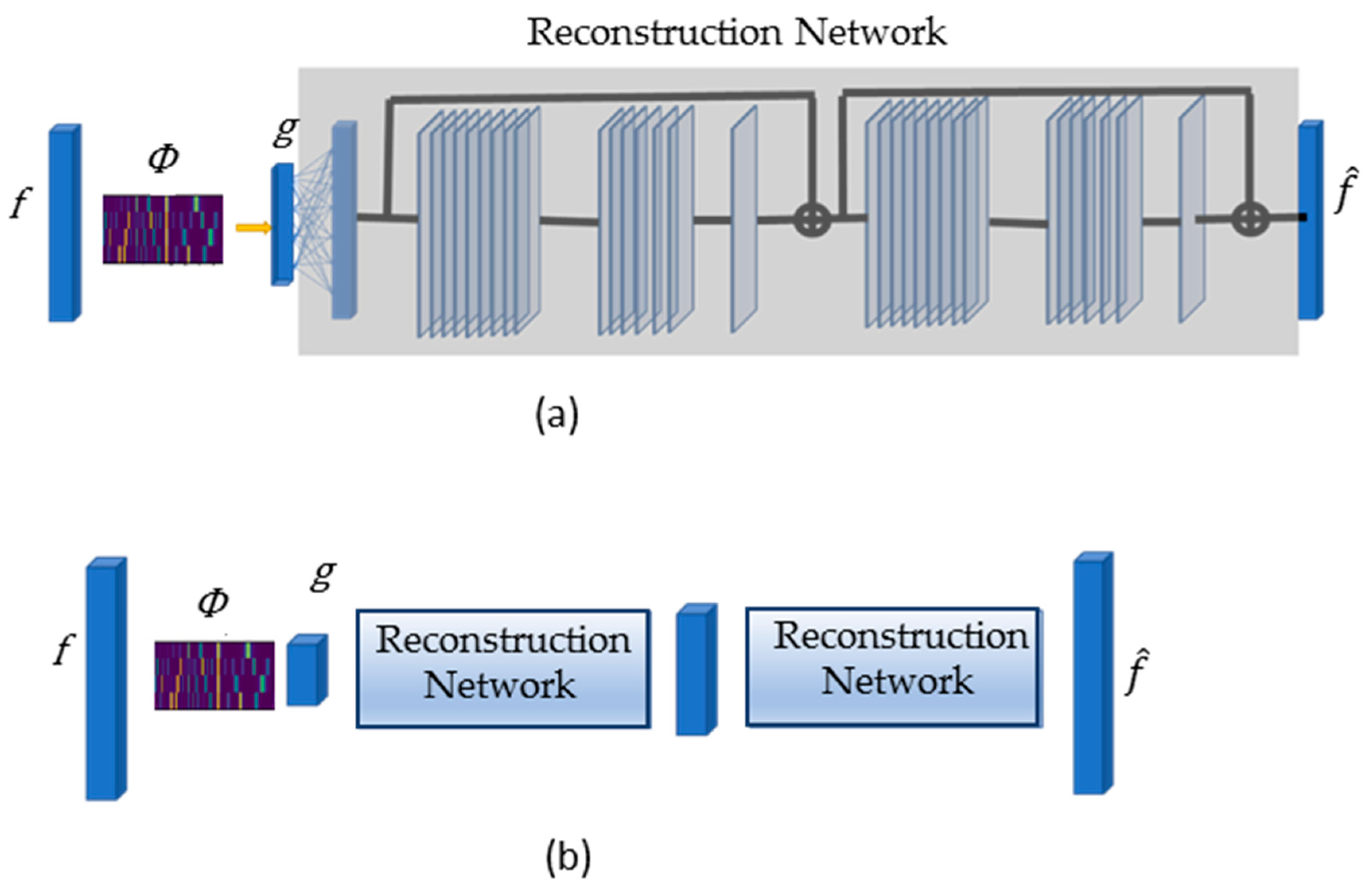
Figure 4a schemes the basic structure of the reconstruction DNN. The first layer of the reconstruction DNN is a fully connected layer that has $N_{\lambda }$ nodes as the $N_{\lambda }$ spectral bands in the label of the spectrum. This layer is followed by batch normalization and a ‘Relu’ activation function. The layer provides a first approximation of the spectrum. The first approximation is followed by a train of residual blocks, where each block consists of 3 convolutional layers and a skip connection, as shown in Figure 4a. The first layer has 64 kernels of size 9, the second layer has 32 kernels of size 1, and the third layer has 1 filter with a kernel consisting of 7 elements. Each layer is followed by batch normalization and a ‘Relu’ activation function. The last layer of the reconstruction DNN is a convolutional layer with 1 filter, which has 1 element and no activation function. Because the task of the reconstruction network is to reconstruct a high-dimensional space from a very small dimensional space, this task is challenging. The transformation of a compressed spectrum $g$ to a fully high-dimensional spectrum $\widehat{f}$ is hard because it is an ill-posed problem, where the compressed signal $g$ is transformed from a narrow subspace to a wider subspace. To mitigate this, we employ a progressive reconstruction approach inspired by the progressive upsampling super-resolution algorithms [44]. Our network upsamples the signal in 4 steps to intermediate sizes and upsamples it again to the final size of the original spectrum, where each step has a train of 5 residual blocks. The number of subnetworks is a hyperparameter of the system. Figure 4b shows 2 steps of a progressive upsampling network.

2.6. Loss Function and Metrics for the PyCAE

We use the mean-square-error (MSE) as the loss function of the PyCAE to reduce the differences between sample pairs (input–label) from the training set in the training phase. The MSE is defined as follows:

$$MSE\left(\widehat{f},f\right)=\frac{1}{n}{\displaystyle \sum }_{i=1}^n\parallel {\widehat{f}}_i-f_i\parallel {}^2$$

(12)

where $n$ is the number of spectral bands in the signal $f\in {ℝ}^{N_{\lambda }}$, and $\widehat{f}\in {ℝ}^{N_{\lambda }}$ is the estimation of signal $f$.

To evaluate the reconstruction performance, we use two widely used metrics:

(1)

Structural similarity index measure (SSIM) [45] to assess the similarity between the structure of the estimated signal to the label as follows:

$$SSIM\left(\widehat{f}, f\right)=\frac{\left(2{\mu }_{\widehat{f}}{\mu }_f+c_1\right)\left(2{\sigma }_{\widehat{f}f}+c_2\right)}{\left({\mu }_{\widehat{f}}^2+{\mu }_f^2+c_1\right)\left({\sigma }_{\widehat{f}}^2+{\sigma }_f^2+c_2\right)},$$

(13)

where $\widehat{f} and f$ are the estimated and original spectrum, respectively; ${\mu }_{\widehat{f}} and {\mu }_f$ are the averages of the estimated and original spectrum, respectively; ${\sigma }_{\widehat{f}}^2 and {\sigma }_f^2$ are the variances of the estimated and original spectrum, respectively; and ${\sigma }_{\widehat{f}f}$ is the covariance of the estimated and original spectrum.

$c_1={\left(k_{1}L\right)}^2 and c_2={\left(k_{2}L\right)}^2$ are two variables to stabilize the division with a weak denominator, $L$ is the dynamic range of the spectral bands, and $k_1 and k_2$ are constants where $k_1=0.01$ and $k_2=0.03$ by default.

(2)

Spectral angle mapper (SAM) [46] evaluates the spectral information preservation degree between the label to the reconstructed spectrum:

$$SAM\left(\widehat{f},f\right)=co{s}^{-1}\left(\frac{\langle \widehat{f}, f\rangle }{{\parallel \widehat{f}\parallel }_2{\parallel f\parallel }_2}\right),$$

(14)

where $\widehat{f} and f$ are the estimated and original spectrum, respectively.

3. Results

3.1. Training Details

To train the PyCAE for spectra reconstruction, we need to initialize the etalon gaps parameters for the activation function according to Equations (4) and (5) The reflectivity of the mirrors is $R~0.8$; hence, the finesse is $F~80$. We take the incident angle $\alpha$ to be $0^{°}$, and the refraction index $n$ is taken to be the BK7 refractive index for each band, depending on the HS cube dataset under analysis.

We used the ADAM optimizer with a learning rate of 0.001 and a learning rate scheduler that reduces the learning rate by a factor of $e^{-0.1}$ after the 3 first epochs.

We trained the PyCAE on two common remote sensing HS cube datasets, Pavia center, and Salinas valley from [39], and evaluated the model on their validation set. We also evaluated its generalization on another HS cube; we evaluated the performance on the Pavia University dataset with the model trained on the Pavia center dataset.

3.1.1. Datasets—Pavia Center and Salinas Valley

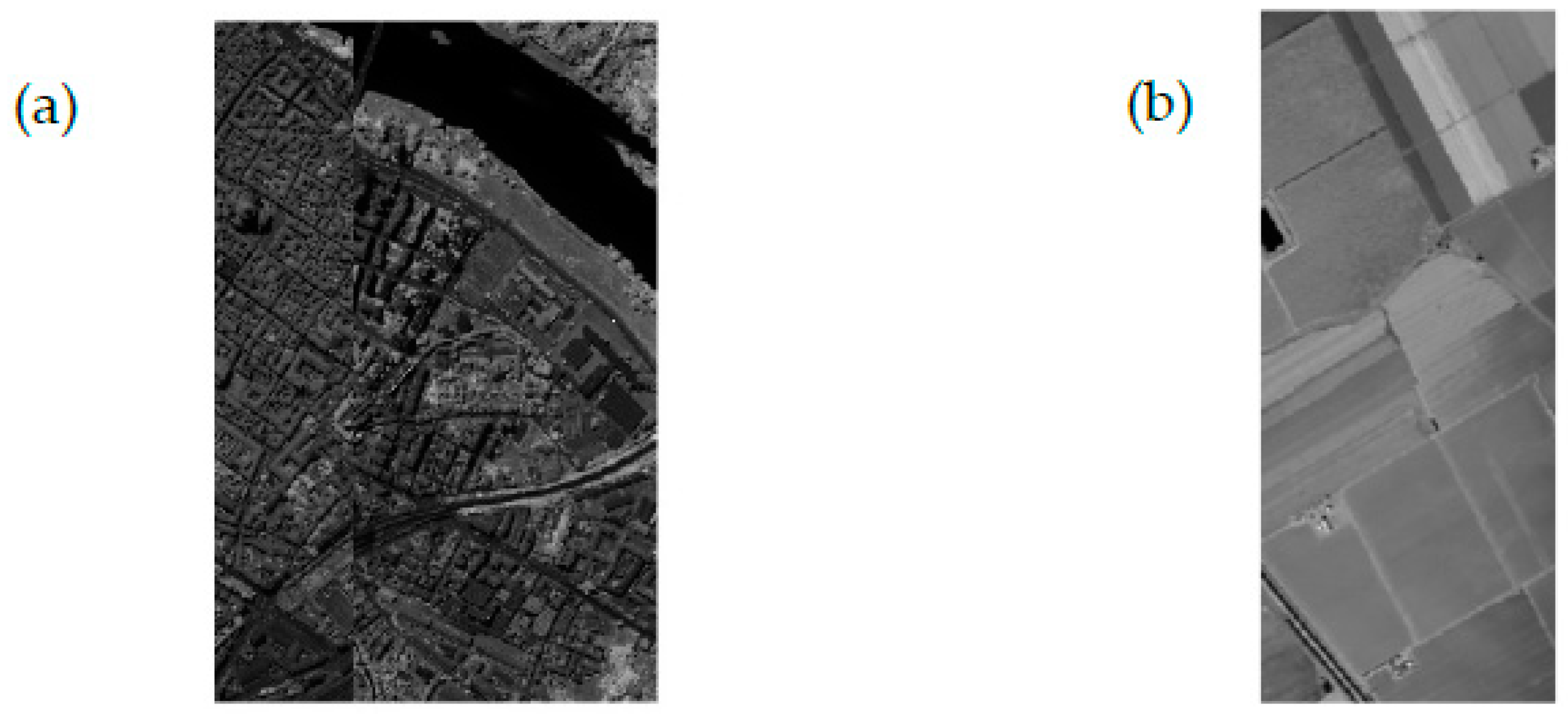
The Pavia center HS cube from [39], consists of two concatenated images of scenes that were acquired by the ROSIS sensor over Pavia center, Italy, with 102 spectral bands from $430 \mathrm{nm}$ to $850 \mathrm{nm}$ and with $1096\times 1096$ spatial pixels as shown in Figure 5. The spectra intensity was normalized to be between 0 and 1. The dataset was augmented by injecting Gaussian noise with standard deviation (STD) $\sigma =0.004$. Then, the HS cube was divided into a training set, which includes the spectra at 70% of the pixels, and a test set, which includes 30% of the pixels.

The Salinas scene from [39], was acquired by the AVIRIS sensor over Salinas Valley, California, with 224 spectral bands from $400 \mathrm{nm}$ to $2500 \mathrm{nm}$ and with $512\times 217$ spatial pixels. The spectra intensity was normalized to be between 0 to 1. The dataset was augmented by injecting Gaussian noise with standard deviation (STD) $\sigma =0.001$. Then, the HS cube was divided into a training set, which includes the spectra of 70% of the spatial pixels, and a test set, which includes 30% of the pixels.

The data of the Pavia center dataset has a wider variance than that of the Salinas valley dataset. In Section 3.3, Section 3.4 and Section 3.5, it can be seen that very few spectra in the dataset are needed to reconstruct the Salinas valley dataset (only 111,104 spectra in the HS cube) with better reconstructions than in the Pavia center and Pavia University (Section 3.2.) datasets (Pavia center includes 1,201,216 spectra in its HS cube), even though its compression ratio is twice smaller. This is due to the tight variance of its data compared to the variance of spectra in the Pavia center and Pavia University datasets.

3.1.2. Pavia University—Generalization Evaluation

In Section 3.1.1, we trained the PyCAE on 70% spectra of one dataset (Pavia center or Salinas valley) and validated and tested it on the remaining 30% spectra. Because many of the spectra are from the same materials under evaluation, they are almost the same, with small deviations inside each group of materials. For this reason, they show a particularly good reconstruction performance.

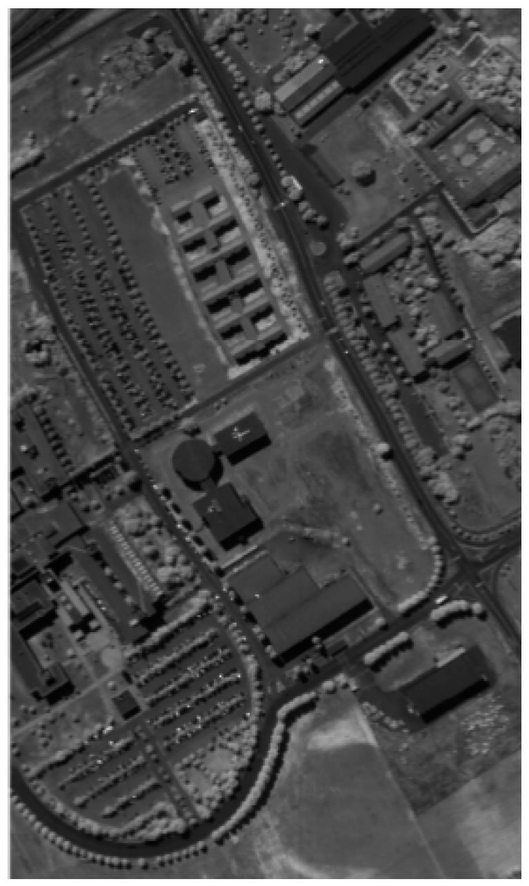
To evaluate the generalization of the PyCAE on a complete unseen dataset, we used the Pavia University dataset from [39] (Figure 6) and consists of a spatial resolution of $610\times 610$ pixels as a test set that didn’t participate in the training phase. Since the Pavia University HS cube was acquired in the same spectral range $\left(430 \mathrm{nm}–850 \mathrm{nm}\right)$ as the Pavia center HS cube, we evaluated the PyCAE that was trained on the Pavia center dataset with the Pavia University dataset.

3.2. The Optimized SpLMs

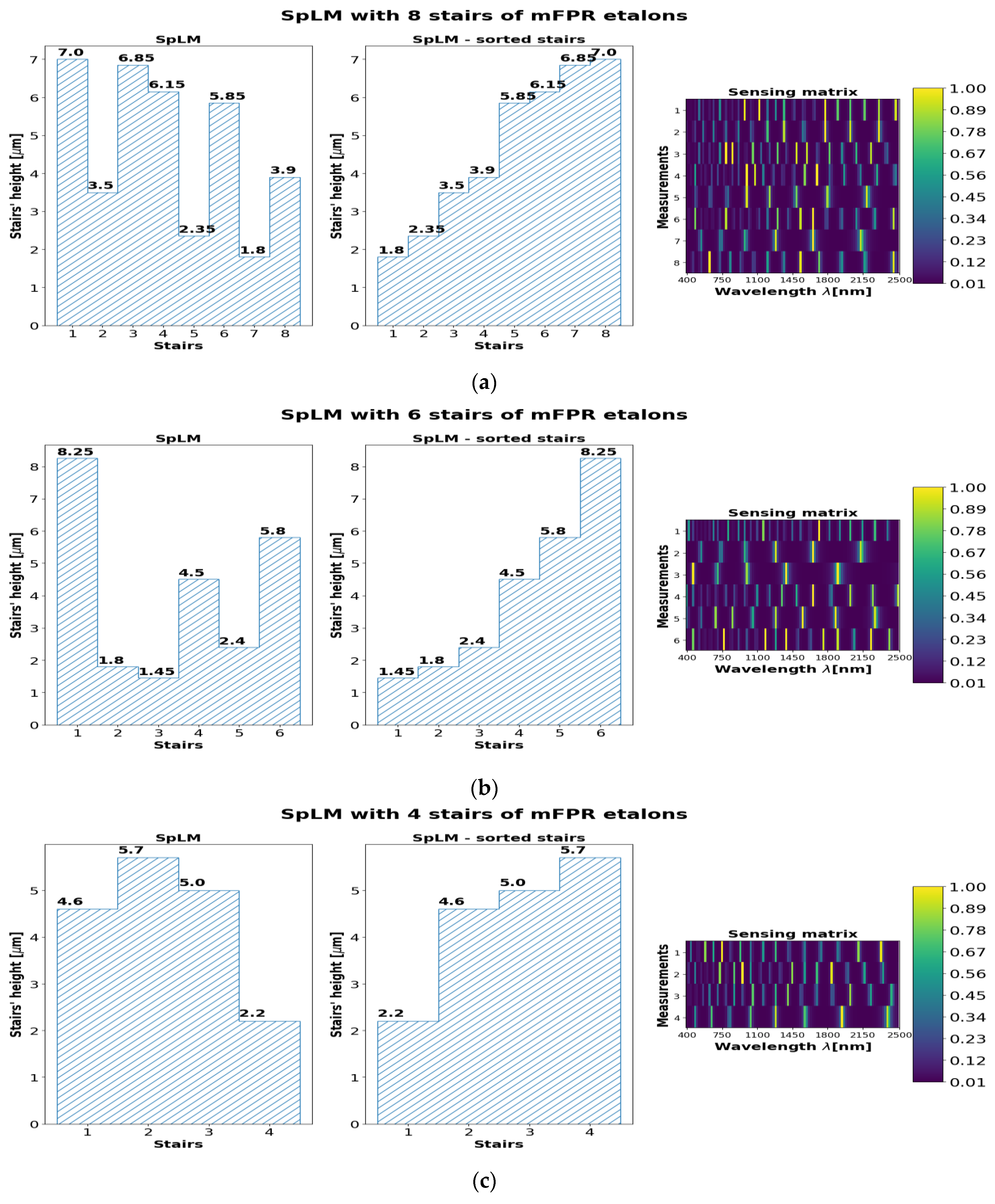
During the training, the SpLM’s geometries were optimized for each dataset and specifically for each version of the PyCAE, where each version has a different number of mFPR stairs. Accordingly, the compatible sensing matrices were optimized. After the optimization, the order of the stairs of the SpLM can be sorted in an increasing order of heights to mitigate the manufacturing process. Then, the resulting measures from the sensor must be registered to the decoder (reconstruction DNN) in the same order it was optimized. As an example, Figure 7 shows the height profile of the learned SpLMs and their respective sensing matrices of the Pavia center for each configuration. The learned profiles of the SpLMs with eight, six, and four staircases are shown on the left-hand side. The SpLMs with the sorted staircase are shown in the center. On the right-hand side of Figure 7, the respective sensing matrix, ${\varphi }_{CS}$, is shown. Each row in the sensing matrix represents the spectral transmission of the mFPR realized in each stair. It can be seen that shallow stairs have low-frequency modulation, while deep stairs have high-frequency modulation. The number of stairs determines the number of rows in the sensing matrix, M, and thus the number of different modulated measurements.

3.3. The Reconstruction DNN

The decoder of the PyCAE (Figure 4) is the software part used for HSI reconstruction, and as such, we report here its running speed on a GPU and its number of parameters. The runtime of the reconstruction DNN implemented by the Tensorflow 2 framework on Nvidia^® RTX 3090 TI GPU is 32 msec., both for PyCAE that was trained on the Pavia center dataset and for the PyCAE that was trained on the Salinas valley dataset. It can be seen that the run time is much shorter than that of common iterative algorithms [7].

The reconstruction DNN (i.e., the decoder of PyCAE), which was trained on the Pavia center dataset, has 672,201 trainable parameters and 4508 nontrainable parameters (total of 676,709 parameters) for PyCAE with 4 measurement configurations, 689,519 trainable parameters and 4516 nontrainable parameters (total of 694,035 parameters) for PyCAE with 6 measurement configurations, and 706,827 trainable parameters and 4524 nontrainable parameters (total of 711,351 parameters) for PyCAE with 8 measurement configurations.

The decoder of PyCAE, which was trained on the Salinas valley dataset, has 1,402,809 trainable parameters and 5240 nontrainable parameters (total of 1,408,049 parameters) for PyCAE with 4 measurement configurations, 1,420,635 trainable parameters and 5248 nontrainable parameters (total of 1,425,883 parameters) for PyCAE with 6 measurement configurations, and 1,438,425 trainable parameters and 5256 nontrainable parameters (total of 1,443,681 parameters) for PyCAE with 8 measurement configurations.

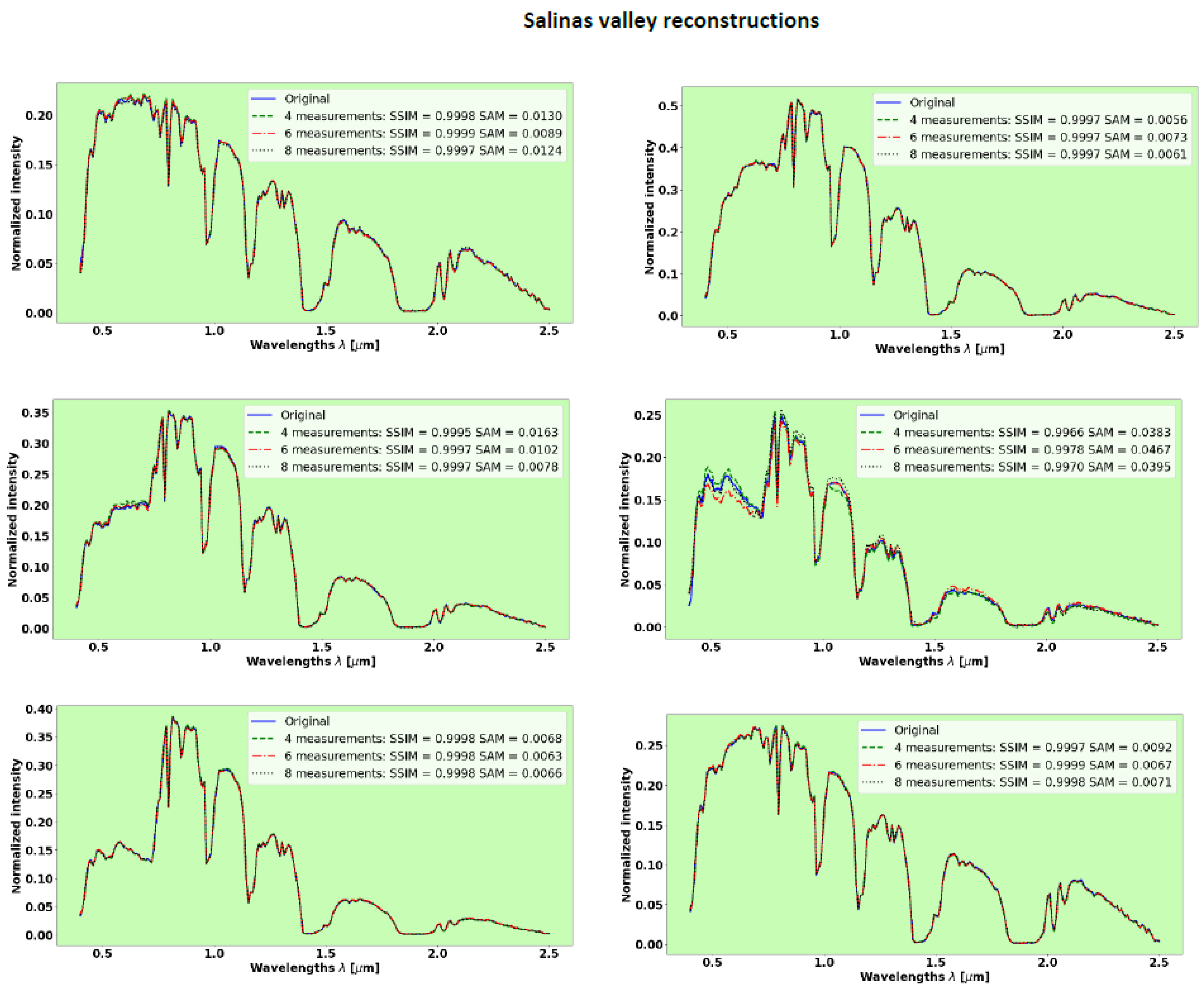
3.4. Salinas Valley

Figure 8 shows the results of spectra reconstruction with 224 spectral bands in the visible-light and SWIR domains evaluated with 8, 6, and 4 measurements. The reconstructions of the Salinas valley show excellent performance.

Table 1. The metrics of SSIM and SAM on the test set for configuration of 8 measurements, 6 measurements, and 4 measurements.

	8 Measurements	6 Measurements	4 Measurements
SSIM	0.9996	0.9913	0.9995
SAM	0.0106	0.0755	0.0138

shows the SSIM and SAM metrics evaluated over the entire test set.

3.5. Pavia Center

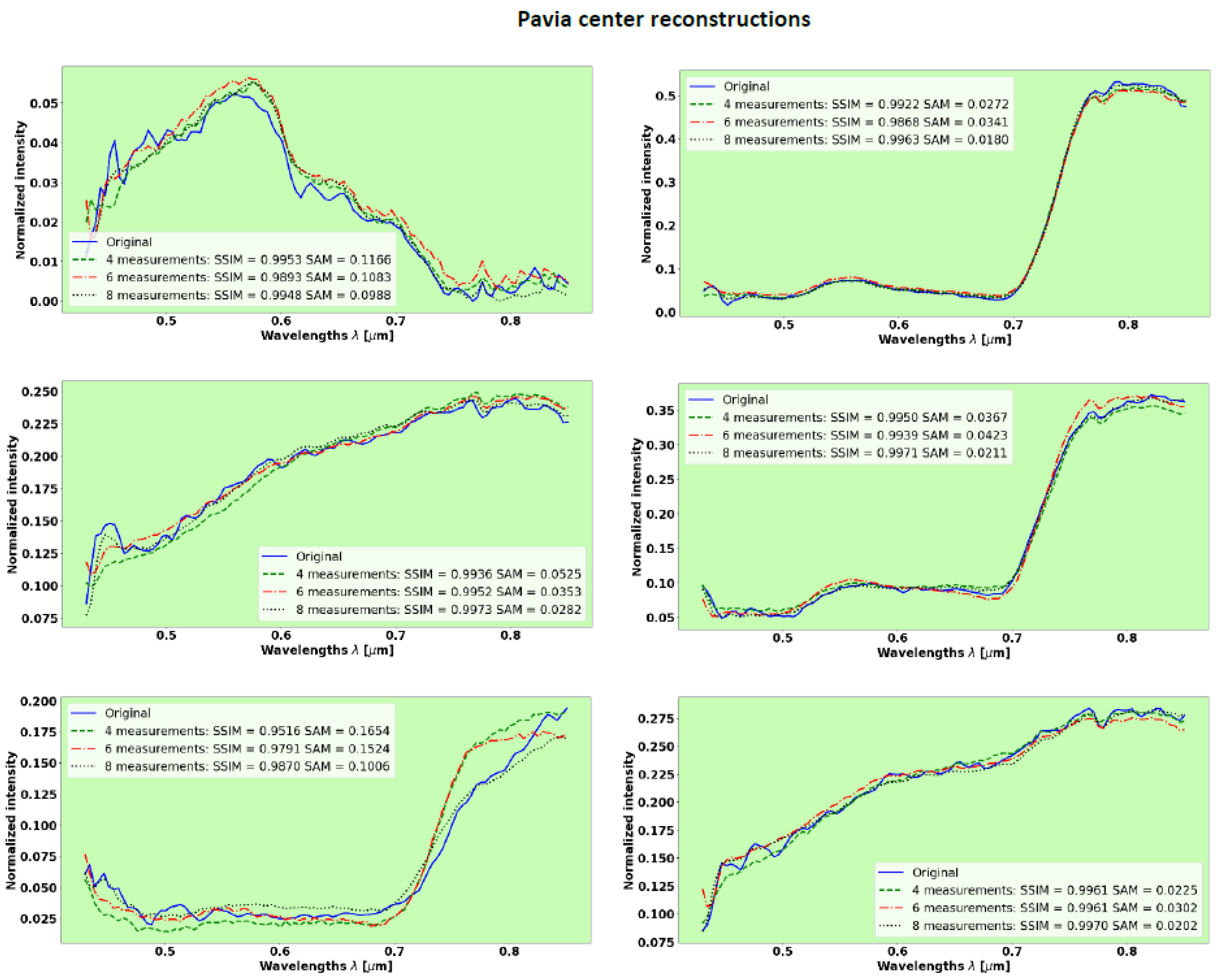
Figure 9 shows representative results of spectra reconstruction with 102 spectral bands, evaluated with 8, 6, and 4 measurements.

Table 2. The mean SSIM and mean SAM over the validation/test set of Pavia center for 3 configurations (8 measurements, 6 measurements, and 4 measurements).

	8 Measurements	6 Measurements	4 Measurements
SSIM	0.9941	0.991	0.9909
SAM	0.05515	0.06891	0.07346

summarizes the results of the mean values for SSIM and SAM over the validation/test set.

3.6. Generalization—Pavia University

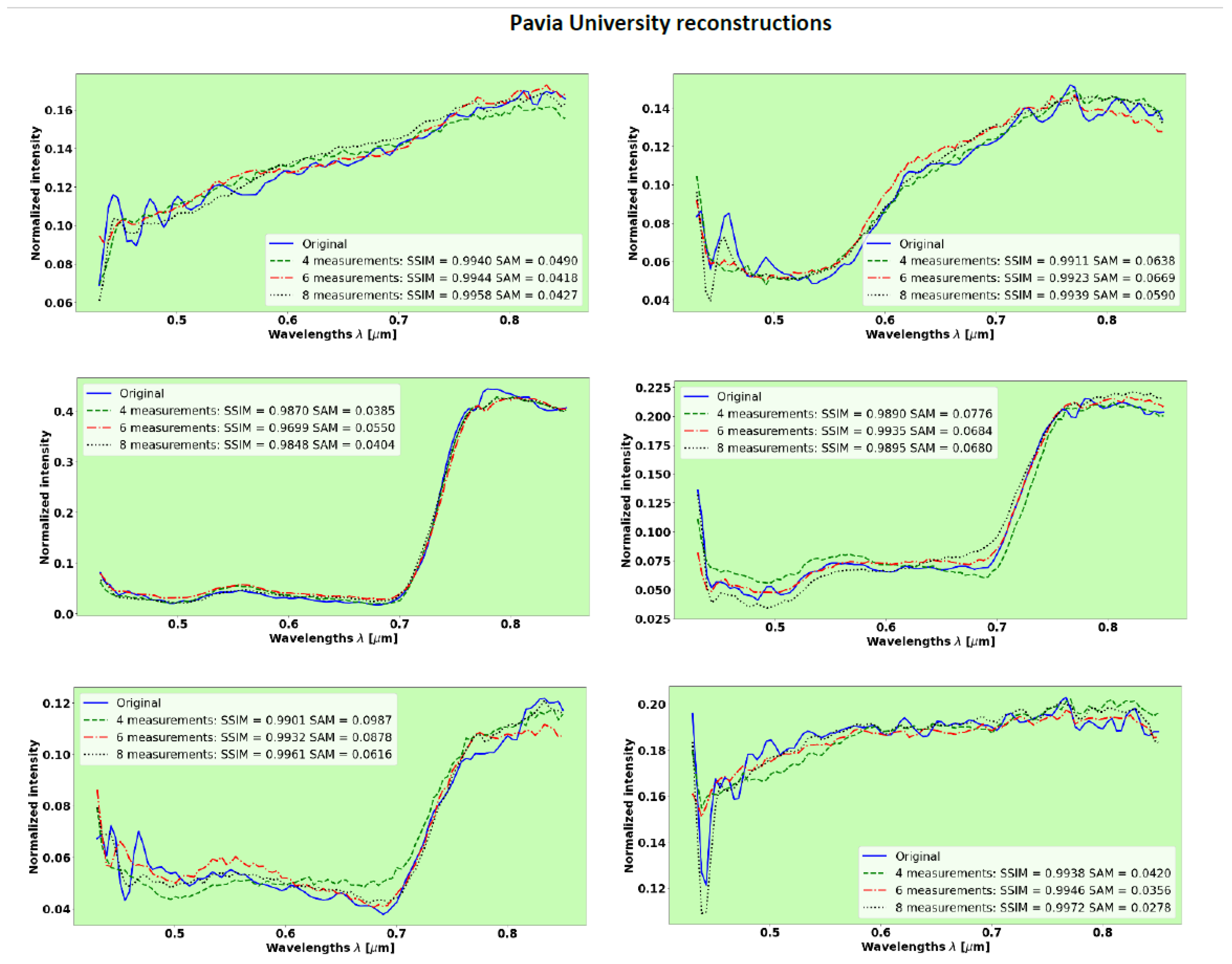
The Pavia center dataset was augmented by adding noise to let the PyCAE evade overfitting. Also, it was divided into 70% for the training set and 30% for the validation/test set. In this section, we evaluate the PyCAE trained on the Pavia center dataset to predict spectra from the Pavia University dataset, which was acquired by the same spectral imaging system on a different scene (Figure 6). Figure 10 shows the results of spectra reconstruction with 103 spectral bands, evaluated with 8, 6, and 4 measurements.

Table 3. The mean SSIM and mean SAM over the dataset of Pavia University for 3 configurations (8 measurements, 6 measurements, and 4 measurements).

	8 Measurements	6 Measurements	4 Measurements
SSIM	0.99210	0.9921	0.9823
SAM	0.04746	0.0484	0.07484

summarizes the results of the mean values for SSIM and SAM over the Pavia University test set. This test set was not introduced to the PyCAE during the training process, which was performed on the Pavia center dataset. It can be seen in Figure 10 and Table 3 that the reconstructions of unseen spectra from the Pavia University test set exhibit similar performance obtained with the validation set from the Pavia center.

3.7. Robustness to Quantization Noise

The SpLM modulates the incident light reaching the sensor, but the sensor adds various kinds of noise. Quantization noise is inherently part of the sensing process, and it depends on the number of bits per pixel. It can distort the compressed measurements, which the reconstruction of the spectrum relies on. Here, we evaluate the impact of quantization noise that cannot be avoided in any digital sampling process of a continuous signal.

We normalized the intensity of spectra in both the Pavia center and Salinas valley datasets in the range of $R=\left[0,1\right]$. To evaluate the impact of quantization noise on the reconstruction, we evaluate the quantization impact on sensors that have pixels with $b=16, 12, 10$, and 8 bits, so the number of quantization levels $L=2^b$, is 65,536, 4096, 2048, and 256, respectively.

The quantization noise (QN) of the compressed spectrum $g$ is:

$$QN~U\left[-\frac{\Delta }{2}, \frac{\Delta }{2}\right],\hspace{1em}\hspace{1em}\Delta =\frac{\max \left(g\right)}{L}$$

(15)

where $b$ is the number of bits in a pixel, $g$ are the compressed measurements and $U$ is the uniform distribution [47].

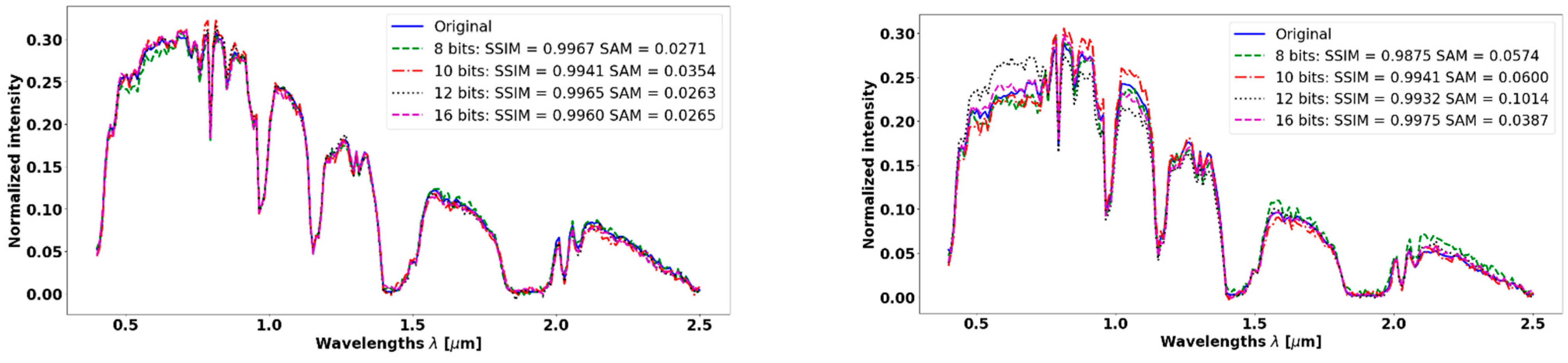
Figure 11 demonstrates the robustness of the PyCAE to these levels of quantization noise and

Table 4. The metrics of SSIM and SAM on the test set for quantization noise of 4 measurements with 16 bits, 12 bits, 10 bits, and 8 bits.

	16 Bits	12 Bits	10 Bits	8 Bits
SSIM	0.99922	0.9922	0.9892	0.9873
SAM	0.03934	0.04092	0.04541	0.05196

summarizes the mean SSIM and the mean of SAM over the Salinas Valley dataset.

4. Conclusions

The PyCAE was trained on the Pavia center dataset with $\frac{8}{102}=7.8\%,\frac{6}{102}=5.9\%$, and $\frac{4}{102}=3.9\%$ compression ratios. It was also trained on the Salinas valley dataset with $\frac{8}{224}=3.6\%, \frac{6}{224}=2.7\%$, and $\frac{4}{224}=1.8\%$ compression ratios. The PyCAE generalization was evaluated on 100% of the Pavia University dataset, by a PyCAE that was trained on 70% of the Pavia center dataset. We found that even at such high compression ratios, our method exhibited excellent reconstructions with an average SSIM above 0.99 and average SAM below 0.07. A similar performance was also obtained on the generalization test on the Pavia University dataset.

Augmenting the datasets by adding exceedingly small normal noise with variation $\sigma =4\times {10}^{-4}$ mitigates overfitting and gives much better results.

The robustness to quantization noise of PyCAE was evaluated on the Salinas valley dataset. The evaluation was performed on typical sensor quantization depths (16 bits, 12 bits, 10 bits, and 8 bits), yet we see excellent results with an average SSIM greater than 0.98 and SAM smaller than 0.071.

PyCAE has proved to be a very efficient optimizer for the design and optimization of SpLM made of a set of mFPRs with different depths for a compressive HSI platform. Moreover, PyCAE can be used as a concept for the optimization of many other signal sensors when the physics model of the sensor is mathematically well defined.

We also presented a new compressive HSI for airborne and spaceborne platforms that benefit from high optical throughput together with reduced bandwidth and storage requirements. This HSI platform, optimized by the PyCAE, is superior to the HSI with wedge-shaped LCC as its SpLM, because it compresses the HS cube by a factor of up to 56:1.