Continual Contrastive Learning for Cross-Dataset Scene Classification

Abstract

With the development of remote sensing technology, the continuing accumulation of remote sensing data has brought great challenges to the remote sensing field. Although multiple deep-learning-based classification methods have made great progress in scene classification tasks, they are still unable to address the problem of model learning continuously. Facing the constantly updated remote sensing data stream, there is an inevitable problem of forgetting historical information in the model training, which leads to catastrophic forgetting. Therefore, we propose a continual contrastive learning method based on knowledge distillation and contrastive learning in this paper, which is named the Continual Contrastive Learning Network (CCLNet). To overcome the problem of knowledge forgetting, we first designed a knowledge distillation module based on a spatial feature which contains sufficient historical knowledge. The spatial and category-level knowledge distillation enables the model to effectively preserve the already learned knowledge in the current scene classification model. Then, we introduced contrastive learning by leveraging the comparison of augmented samples and minimizing the distance in the feature space to further enhance the extracted feature during the continual learning process. To evaluate the performance of our designed model on streaming remote sensing scene data, we performed three steps of continuous learning experiments on three datasets, the AID, RSI, and NWPU datasets, and simulated the streaming of remote sensing scene data with the aggregate of the three datasets. We also compared other benchmark continual learning models. The experimental results demonstrate that our method achieved superior performance in the continuous scene classification task.

1. Introduction

Remote sensing scene classification tasks can be considered to assign semantic labels to high spatial resolution (HSR) image patches. According to the different spatial distributions and combinations of objects, remote sensing scenes can be divided into semantic categories which contain specific semantic information, such as airport, forest, resort and tennis court, etc. The fundamental scene classification task has led to a wide range of applications such as urban planning [1], environmental monitoring [2], disaster detection [3], and object recognition [4,5].

Over the past few years, remote sensing scene classification has achieved significant improvements. Several researchers have developed various well-performed methods for remote sensing scene classification tasks. Especially, deep-learning-based methods take full advantage of deep feature extraction and classification to achieve state-of-the-art performance in scene classification. However, with the development of real-time earth observation technology in the remote sensing field, extensive new remote sensing imageries are continuously acquired from different satellites. It is quite difficult to directly delineate ever-increasing new images accurately with pre-trained models as the significant variation (such as spatial resolution, and imaging angles) comes from different sensors. Moreover, the existing models usually fail to continually update with non-independent identically distribution (non.i.i.d) streaming data and result in a catastrophic forgetting of the previous knowledge for remote sensing classification. Thus, it is critical to preserve the knowledge learned by the old model while extending the new task learning.

Currently, several studies adopt pre-trained models to continually update with the consecutive tasks for cross-dataset scene classification, for example, Lima et al. [6] used a model pre-trained on ImageNet and then applied it to the new remote sensing scene classification task. However, pre-trained model features based on natural images cannot be directly transferred to remotely sensed images due to the significant differences. To address the cross-domain problem, several transfer-learning-based methods are employed to perform scene classification tasks. For example, Li et al. [7] fine-tuned with a few shot samples and achieved favorable performance on scene classification tasks. Song et al. [8] adopted domain adaptation to maintain the consistency of source and target domain features in the subspace and effectively improved the scene classification. Although transfer learning effectively transfers knowledge from the source domain to the target domain, forgetting the previous knowledge of earlier tasks is still inevitable for continuous learning tasks, especially when the models are constantly being updated.

In order to tackle the catastrophic forgetting problem in the streaming scene classification tasks, continual learning or life-long learning is introduced which enables the model to adaptively learn from tasks without a predefined number of samples and categories. The existing methods are mainly divided into three groups: replay-based methods, regularization-based methods, and parameter-isolation methods [9]. To consolidate already learned knowledge, replay-based methods adopt a strategy that saves the original data or a model that can generate the data to mitigate forgetting. For example, Rebuff et al. [10] developed a training strategy for continual learning via stored historical samples. Kamra et al. [11] proposed a generative dual memory network that could be used to generate pseudo-data for previous information preservation. Similarly, to overcome the model’s forgetting of historical knowledge, Rostami et al. [12] used a generative model to produce pseudo samples with a few samples from the previous tasks, so that the abstract concepts have effectively emigrated from the generative model to the current task. Shin et al. [13] proposed the deep generative replay framework with a “generator” and “solver”, where the “generator” is applied to generate data from the previous task, and the “solver” is then used to handle the current task with generated samples. Verma et al. [14] demonstrate the contribution of their proposed Efficient Feature Transforms in generative models to overcome catastrophic forgetting. Although the replay-based methods obtained favorable results, the additional requirement of storage space and the complexity of training the generative model mean such methods cannot be applied in resource-limited situations. The regularization-based method protects previously learned knowledge by constraint parameter updates which typically add a regularization term to penalize change in critical parameters. Kirkpatrick et al. [15] firstly proposed Elastic Weight Consolidation (EWC), an approach that employed a quadratic penalty term to constrain the update of important weights calculated through the diagonal of the Fisher information matrix. Similarly, Aljundi et al. [16] also proposed a method to preserve important parameters, which is called Memory Aware Synapses (MAS). MAS estimates the importance of each parameter based on the sensitivity of the predicted output function, which effectively prevents valuable parameters from being covered. However, the memorization mechanisms of regularization-based methods show poor performance on discriminate inter-tasks categories. However, the additional loss term that is used to protect consolidated knowledge may lead to a performance trade-off between old and new tasks [17]. The third parameter isolation approaches allocate fixed parameters for each task to prevent model forgetting. This method is also subdivided into dynamic architecture and fixed architecture, depending on whether the model structure changes. For instance, Yoon et al. [18] proposed the Dynamically Expandable Network (DEN), which dynamically expands the capacity of the old model when encountering new tasks. Rusu et al. [19] avoid modifying corresponding sections of previous tasks while extending the model for new tasks. Meanwhile, in the fixed architecture solutions, PathNet [20] and PackNet [21] employ binary masks to restrain parameters of subsets of the network for the specific tasks. However, the parameter-isolation methods still suffer from the problem of parameter independence, which restricts the robustness of complex tasks.

The three schemes mentioned heavily focus on the collection of historical experience, but Lee et al. [22] argued that it still leads to more forgetting due to the restriction of future events. Therefore, to alleviate catastrophic forgetting, they have learned more representative features in the first instance. Inspired by this, obtaining meaningful features within the continual learning process becomes critical to alleviating catastrophic forgetting. For remote sensing scene images, there is a large quantity of land cover types and ground objects covered in the same imagery, and the inter-class similarity and intra-class diversity cause scene classification tasks to be more challenging. In addition, the images acquired from different satellites have the problems of variation in illumination, backgrounds, scale and noise, which further increase the discrepancy of scene images across different datasets. Facing the dramatic variations in images, how to extract discriminative features with limited annotated samples becomes the primary goal.

In order to capture more representative features for continual scene classification, self-supervised, especially contrastive learning has demonstrated the strength of obtaining the intrinsic features. Unlike supervised methods that require numerous manually annotated labels, contrastive learning uses similarity metrics to measure the distance between positive and negative samples after transformation. It brings similar samples too close together and separates distinct samples, by learning invariant features. For instance, Zhao et al. [23] combined scene classification task with contrastive learning, which further improved feature extraction and the generalization of the model. Tao et al. [24] obtained high performance model for scene classification tasks under insufficient labeled samples via introduced contrastive learning and achieved favorable results. Stojnic et al. [25] analyzed the effect of sample size and domain of scene images for training, and their work demonstrated that results of pretrained models by contrastive learning outperform others on scene classification. Therefore, building robust and discriminative feature representations for describing the scenes is the essential component in the cross-dataset scene classification. Although it is possible to strengthen the deep feature obtained through contrastive learning, there is still a restriction in preserving consolidated knowledge over a stream of tasks.

Moreover, due to the similarity of samples among different datasets, it is difficult for the model to reuse the valuable knowledge learned from previous data. The knowledge distillation strategy, especially the distillation of feature-level knowledge and semantic information enables the model to obtain more transferable features effectively. Indeed, the representative feature extraction for continual learning is intended to improve future tasks. However, it still lacks a knowledge retention mechanism to preserve the acquired representative features under streaming tasks. Specifically, the lack of distillation of historical model features, especially for complex remote sensing scene images, results in the learned spatial knowledge becoming unadaptable for future scene classification tasks. The deep and abstract spatial features in the previous model no longer facilitate the learned knowledge retention and eventually leads to forgetting.

Based on the issues mentioned, it is essential to employ contrastive learning to enhance the robustness of the extracted features with the distillation strategy introduced. On the one hand, due to the complex spatial configuration and significant distinctions between different datasets, contrastive learning representations will further enhance the features to boost future learning. On the other hand, the knowledge distillation can transfer valuable learned knowledge to new tasks effectively and optimize scene classification. Especially for the spatial features and class distillation, the catastrophic forgetting could be dramatically alleviated by mimicking the different level features and the final output of the historical model. Hence, we considered applying both contrastive learning and knowledge distillation to guarantee the model acquires robust features while preserving the historically learned knowledge.

In this case, we propose the continual contrastive learning network (CCLNet) for continual scene classification, which contains a deep feature extractor, knowledge distillation mechanism, and contrastive feature enhancement scheme. Firstly, we designed the contrastive loss module through comparing samples with different augmented views which are used to enhance the robustness of features for continual scene classification tasks. Then, we introduced deep spatial feature distillation and class distillation for knowledge preservation by imitating the different level features and outputs of historical models. The integration of the contrastive loss module and the knowledge distillation strategy for continual learning ensures the model captures comparison information under limited annotated samples across different datasets, while further assuring knowledge retention.

The main contributions of the proposed CCLNet are:

(1)

contrastive learning for continual learning enables the model to learn invariant and robustness features of complex scene images under limited annotated samples.

(2)

the designed spatial and class distillation to effectively distill the latent shape and other knowledge of previous model into the current model thus facilitating continual learning.

The remaining parts of the paper are organized as follows: Section 2 introduces related works of this paper. Section 3 describes in detail the proposed method in this paper. Section 4 presents the experimental data and then details the setup of the experiments. Section 5 analyzes and discusses the results of the experiments. Finally, Section 6 provides the conclusion of the paper.

2. Related Work

In this section, we first give an overview of the recent works on scene classification, especially scene classification based on deep learning and contrastive learning. Then, we discuss the contribution of knowledge distillation to the retention of critical historical knowledge for scene classification.

2.1. Deep-Learning-Based Scene Classification

Extracting discriminative features is crucially important for remote sensing scene classification tasks. According to the feature acquisition method, scene classification approaches are divided into low-level, mid-level, and high-level. For example, earlier low-level features such as color histograms, grayscale co-occurrence matrices, and local binary patterns mostly relied on manual assistance. Then, the mid-level methods, such as Bag of Visual Words (BoVW), improved description of features and demonstrated its effectiveness in scene classification. However, encoding the representative high-level feature is still a challenging task due to the inter-class similarity and intra-class diversity of different datasets.

To capture higher-level representative features of scene imagery, deep learning demonstrates a powerful feature extraction capability and has been used intensively in recent remote sensing scene classification. For example, the majority of the deep-learning-based methods achieved optimal performance on remote sensing scene classification tasks. At the beginning, there is a tendency for many researchers to use a convolutional neural network (CNN) for scene classification. For example, Zou et al. [26] proposed a deep-learning-based features selection method that extracts discriminative features for scene classification. However, it is difficult to train a completely new network due to the limitation of computational resources and the cost of acquiring annotated samples. Therefore, some literature starting to extract features by using networks pre-trained on other large-scale datasets, e.g., ImageNet. Marmanis et al. [27] extracts deep features and transfers the knowledge from the previous pre-trained network for scene classification. Hu et al. [28] extract multiscale features and encode these features into global representative image features for scene classification. Similarly, in order to obtain representative features for scene image classification, Chaib et al. [29] combined features from each layer of the pre-trained model to construct robust features. Although the methods previously mentioned have been implemented successfully for scene classification, the problem of feature generalization and stabilization remains, especially when pre-trained on nature images and when the target tasks are remote sensing images. To handle this problem, we use contrastive learning to further enhance the features without sufficient annotated samples.

2.2. Contrastive Learning for Scene Classification

Contrastive learning methods learn robust representations from unlabeled samples by creating positive and negative samples, and thus transfer the learned knowledge to further improve downstream works. For these state-of-the-art contrastive learning models, MoCo [30] and SimCLR [31] currently obtain discriminative features by measuring the similarity between positive and negative samples. Moreover, MoCo-v2 adds a nonlinear layer to enhance features inspired by SimCLR. For SimCLR-v2 [32], a deeper projection head is introduced and better enables feature extraction. Moreover, SwAV [33], BYOL [34], and SimSiam [35] are proposed for a new contrastive learning scheme that does not require negative samples and prevents collapse caused by applying only positive samples. These methods prove that the contrastive learning framework can still obtain robust features without negative sample pairs. Recently, many contrastive-learning-based methods are employed in remote sensing scene classification tasks. Firstly, Tao et al. [24] pre-train a high-performance feature extract model from large unlabeled images and demonstrate that contrastive learning outperforms pre-training on the ImageNet dataset. Gómez et al. [36] present MSMatch, which is combined with self-supervised contrastive learning, where the learned knowledge can even be effectively transferred to scene classification tasks. Hence, contrastive learning is proven to obtain more transferable features and overcome the problem of knowledge migration through pretraining on remote sensing scene datasets. In addition, Li et al. [37] proposed SCL-MLNet, which employs contrastive learning to enhance feature extraction ability for few-shot remote sensing scene classification. Huang et al. [38] introduce the STICL approach, which transfers invariant spatial-temporal features to another dataset via a contrastive learning mechanism. The above studies demonstrate that contrastive learning effectively improves scene classification performance; this study will therefore leverage contrastive learning to further enhance the model feature extraction.

2.3. Knowledge Distillation for Continual Contrastive Learning

Many studies have explored knowledge distillation to prevent model forgetting. Hinton et al. [39] firstly promote the performance of knowledge distillation strategies on image classification, which use the softened output of the previous teacher model to transfer knowledge to the student model. Similarly, Müller et al. [40] introduce label smoothing while using the logits output of the teacher model to transfer knowledge. Moreover, not only the information in the final output layer of the teacher network is used, but the hidden knowledge in the middle layers is also exploited. For instance, Romero et al. [41] additionally employ intermediate layers of the teacher model as hints for knowledge distillation. Zagoruyko et al. [42] enable the student model to mimic the attention maps of the teacher model. Ji et al. [43] leverage an attention-based network that obtained multiple levels of features to learn feature similarities for knowledge transfer.

As the knowledge distillation strategy can effectively transfer the learned knowledge from the previous model to the current model, this has been widely adopted in continual learning. For example, Li et al. [44] preserve already learned knowledge through their proposed LwF method, in which knowledge distillation is used. In LwF, the model trained on the previous task will be used as a teacher network to further train for the current task. Castro et al. [45] use cross-entropy loss to learn a new task and use a distillation loss to retain knowledge learned from historical data. In [46], a bias correction for the last classifier layer is used to avoid the overwriting of old knowledge by new knowledge. Hence, we introduced knowledge distillation to mitigate forgetting and integrated it with continual contrastive learning.

3. Methods

To allow the current classification model to be used across different remote sensing scene datasets, we propose a continual contrastive learning approach to distillate the spatial and class knowledge and avoid forgetting. We use a deep-learning-based feature extractor to acquire deep feature representation of the scene images and obtain outputs of the last classifier layer. After that, intermediate features and logits output matching between the new and old model as the distillation strategy to migrate the previously learned knowledge to the current model. In addition, contrastive learning is introduced to further enhance the robustness of extracted features during learning from streaming scene datasets. The overall architecture of our model shown in Figure 1.

3.1. Spatial Feature and Class Matching Distillation for Knowledge Preservation

Consider that there are T-step continual scene classification tasks, which mainly contain the first initial task and the current T-step task. Generally, most scene images contain both annotated and unannotated data. We presume that the continual scene classification task is built on a streaming dataset $D=\left\{D_L^t,\left.D_u^t\right|t\in \left(1,\dots T\right)\right\}$, where t is the t-step task, $D_l$ and $D_u$ represent the labeled scene data set and unlabeled data set, respectively. For the t step scene images dataset $D_L=\left\{\left.\left(x_i,y_i\right)\right|i\in \left(1,\dots ,N\right)\right\}$, which contains N samples, $x_i$ and $y_i$ denote the scene image and the corresponding ground-truth label of this sample, respectively. The dataset $D_u=\left\{\left.x_j\right|j\in \left(1,\dots ,M\right)\right\}$, which denotes scene images without any label, usually satisfies $N\ll M$. Except for the first dataset, which is used to train the base model, the following data will be used for the continual scene classification task. At the t-th learning step, while the model learns new knowledge from the current scene data set with C categories. The previous knowledge of K categories learned in the t-1 step will be migrated to the current model by knowledge distillation. Specifically, samples are selected from the historical data set for the current model training, so the current t-th training data can be represented as $D_{t-th}={\left\{\left(x_i,y_i\right)\right\}}_0^{K+C}$. Hence, we designed a CNN-based model to extract deep features used for knowledge transfer. The scene images can be used as input to the model to extract deep spatial features of scene imagery and obtain the output of the final classifier layer. In addition, contrastive learning is used to further enhance the robustness of acquired scene features with the available unlabeled data. In this case, the performance of scene classification models for complex remote sensing scene images will be further improved.

Acquiring representative features of scene images through deep neural networks is critical to outperforming traditional methods. To obtain latent spatial information from a large number of complicated images, a deep CNN module is introduced. The regular CNN architecture consists of a series of convolutional layers, pooling layers and nonlinear layers. For feature extraction, the convolutional layer is the most important. The first convolutional layer obtains relatively low-level representations of the scene images, and higher-level features will then be extracted by the deepening of the layers as they become deeper. The nonlinear layers are connected after the convolutional layers to provide nonlinear signatures for the deep model. After that, the pooling layer, which usually uses maximum pooling, is used to reduce the dimension of the representation. Specifically, given an input scene image $x_i$, the process of extracting spatial context information can be expressed as

$$f_l=\sigma \left({\displaystyle \sum }_{i=1}^k{W}_i^l*f_{l-1}\left(x_i\right)+W_b^l\right)$$

(1)

where $*$ represents convolution operation, $f_l$ denotes the current l-th feature map, $f_{l-1}$ is the feature map of previous l − 1-th layer. To simplify the expression of the model parameters, we set $W_i^l$ as the weight matrix of the l-th layer and $W_b^l$ as the corresponding biases. $\sigma \left(·\right)$ denotes the non-linear activate functions after the convolution operation which is rectified to a linear unit (ReLU).

In the scene classification CNN, the pooling operation is adopted to minimize the unnecessary information for deep spatial features and further decrease the number of parameters to be trained. We compute the pooled feature will be

$$f_l=maxPool\left(\sigma \left({\displaystyle \sum }_{i=1}^k{W}_i^l*f_{l-1}\left(x_i\right)+W_b^l\right)\right)$$

(2)

where $maxPool\left(·\right)$ represents the max pooling operation for current l-th layer, which filters out the useless information and allows the obtained spatial features to be more robust.

With the above process, the spatial features of scene images from different levels are acquired. In continuous learning, the consistency of deep features between the old and new models means that the model can be considered to retain the knowledge effectively. To prevent catastrophic forgetting, feature-based distillation is applied to transfer historical knowledge to the current model. Specifically, the distance between the extracted features of the old and new models is measured to enable the performance of the current model to fit the historical model. Usually, the cosine similarity is acquired by calculating the cosine of the angle between two features in a feature space. Hence, for different hierarchical features of scene images extracted by the old and new models, the cosine-similarities of vector representation of single scene image x can be calculated as

$$co{s}_{\_}s\mathrm{i}m\left(f_{old},f_{new}\right)=\frac{{\Sigma }_{\mathrm{i}=1}^n{F}_{old}^{ }\left(x\right)\times F_{new}^{ }\left(x\right)}{\sqrt{{\Sigma }_{i=1}^n{\left(F_{old}^{ }\left(x\right)\right)}^2}\times \sqrt{{\Sigma }_{i=1}^n{\left(F_{new}^{ }\left(x\right)\right)}^2}}$$

(3)

where $F_{old}^{ }\left(x\right)$ and $F_{new}^{ }\left(x\right)$ represent the features acquired by the old and new models from the same image. Therefore, the spatial feature distillation for the scene samples from the same batch is expressed as

$$Spatia{l}_{\_}distill=\frac{1}{NL}{\displaystyle \sum }_{n=1}^N {\displaystyle \sum }_{L=1}^{L}co{s}_{\_}s\mathrm{i}m\left(F_{old}^l\left(x_n\right),F_{new}^l\left(x_n\right)\right)$$

(4)

where N is the number of training scene images involved in the same batch, and L indicates the number of layers for acquiring features in the model. Thus, in order to protect more knowledge learned from the previous model, the spatial feature distillation loss can be designed to maximize the similarity of features between the old and new models. For easier loss calculation, the final feature distillation loss function is formulated as

$$L_{sp{a}_{\_}distill}=minimize\left(1-Spatia{l}_{\_}distill\right)$$

(5)

Normally, the value of similarity between features is in the range from 0 to 1. The higher the similarity among the feature vectors, the closer the value of cosine similarity is to 1. Therefore, the current model retains previous scene information well as the value of the loss function close to 0.

In addition, not only is the knowledge saved by mimicking the feature map of the historical model, but also the higher-level information can be preserved when the prediction for same scene image of the current model is similar to the previous model. Consequently, to avoid the prediction categories of the recent model for the scene images to be biased towards the new categories, the class loss is designed as

$$L_{class}=\frac{1}{N}{\displaystyle \sum }_{n=1}^N{\left(F_{new}\left(x_i\right)-F_{old}\left(x_i\right)\right)}^2$$

(6)

where N represents the training scene images in a batch, and $F_{new}$ and $F_{old}$ are prediction results of the new and old models for the same scene images, respectively. Compared with feature distillation, it is more efficient to use the output of the last fully connected layer of the model for knowledge transfer.

3.2. Supervise and Contrastive Learning for Knowledge Learning

In continual remote sensing scene classification tasks, besides preserving knowledge of historical data by using knowledge distillation, it is also necessary to learn new knowledge from the new data. The cross-entropy loss function is usually used as a measurement of the probability distribution difference between the model prediction and the ground-true label. Given an input scene image $x_i$ with a corresponding label $y_i$, feed the extracted features to the softmax layer for obtaining the predicted class probability, the process can be described as follows

$$p\left(\widehat{y}=\left.c\right|f\left(x_i\right)\right)=\frac{exp\left(W^{\prime }\cdot f\left(x_i\right)+W_b^{’}\right)}{{{\displaystyle \sum }}_{c=1}^{C}exp\left(W^{\prime }\cdot f\left(x_i\right)+W_b^{’}\right)}$$

(7)

where $\widehat{y}$ represents the prediction of input scene image $x_i$, and C is the total classes for current step classification task. The $W^{\prime }$ and $W_b^{’}$ are the trainable weights and biases for softmax layer. Consequently, the cross-entropy loss for new data learning could be calculated as

$$L_{task}=-\frac{1}{N}{\displaystyle \sum }_{i=1}^N {\displaystyle \sum }_{c=1}^C{y}_c\log \left(p\left(\widehat{y}=\left.c\right|f\left(x_i\right)\right)\right)$$

(8)

where N represents the quantity of training scene images in a batch, and C indicates the total categories of images contained in the current task.

In order to further enhance the feature extraction, self-supervised contrastive learning is adopted. Given a remote sensing scene image x, this can be converted into two images $x^{\mathrm{a}}$ and $x^{\mathrm{b}}$ by two randomly augmented actions such as rotation, crop and brightness adjustment, etc. A batch of unlabeled scene images ${\left\{x_i\right\}}_{i=1}^N$ will be transformed to ${\left\{x_i^{\mathrm{a}},x_i^{\mathrm{b}}\right\}}_{\mathrm{i}=1}^N$. The features obtained from these images will then be mapped to the d-dimension features through a projection layer. This can be described as

$$z_i=g\left(F\left(x_i\right)\right)$$

(9)

where $g\left(·\right)$ represents the feature projection function, and$F\left(·\right)$ indicates that the image is encoded as a deep feature representation. Eventually, the encoded features obtained from the two pairs of transformed images are used to calculate the cosine similarity. The self-supervised contrastive training process by using unlabeled images is illustrated as follows

$$L_{i,j}=-log\frac{exp\left(sim\left(z_i,z_j\right)/\tau \right)}{{\Sigma }_{k=1}^{2N}{1}_{\left[k\ne i\right]}exp\left(sim\left(z_i,z_k\right)/\tau \right)}$$

(10)

where N is the number of training samples for a batch, 2N denotes the number of augmented samples from the same batch, and$sim\left(·\right)$ indicates the calculation of cosine similarity between feature vectors. $z_i$ and $z_j$ denote the features from the same image and can be considered to be a positive pair, while $z_k$ represents features extracted from other images among the same batch. $\tau$ represents temperature parameter. Consequently, the total contrastive loss of the batch can be represented as

$$L_{con}=\frac{1}{2N}{\displaystyle \sum }_{i=1}^N\left(L_{2i-1,2i},L_{2i,2i-1}\right)$$

(11)

To sum up, the final continual learning for remote sensing scene classification can be expressed as follows

$$L=L_{task}+L_{con}+L_{sp{a}_{\_}distill}+L_{class}$$

(12)

The detailed training process of the proposed CCLNet for continual scene classification can be seen in Algorithm 1.

Algorithm 1 The proposed continual contrastive learning for scene classification

Require: Streaming datasets $D_t$ which contained annotated dataset $D_t^L$ and unannotated dataset $D_t^u$ for task T, $t\in 0,1,2,\dots ,T$, $D_0$ represents initial ImageNet dataset the network $F\left(x_i;W_t^{*};W_t^b\right)$, $t=1, 2,\dots ,T$ random initialized parameters $W^{*}$ and $W^b$ sim(·) are cosine similarity of new and old model features for t = 1, 2, …, T do     $D_t$ ⃪ $D_{t-1}$     for s = 0, 1, …, S do         for m = 1, 2, …, M do             sample a mini-batch $B$ from $D_t$             for all $x_i$ $\in B$ do                 feature distillation loss $L_{spa\_dist}$                 class loss $L_{class}$                 cross-entropy loss $L_{task}$                 contrastive loss ${\mathrm{L}}_{\mathrm{con}}$             end for         update previous task parameters $W_{t-1}^{*}$ and $W_{t-1}^b$ and minimize loss function Equation (12)         end for     end for     $W_t^{*}$ ⃪ $W_{t-1}^{*}$     $W_t^b$ ⃪ $W_{t-1}^b$ end for Return model $F\left(x_i;W_t^{*};W_t^b\right)$ for current task T

4. Datasets Description and Experiments Set up

In this section, we detail the dataset used for continual scene classification and experimental setup. We then introduce the method for the evaluation of the effectiveness of the methods in this paper and other benchmark methods.

4.1. Datasets Description

• AID data set: the AID dataset collected from google earth was proposed by Xia et al. [47] in 2016 for aerial scene classification. The large-scale dataset contains 10,000 images in 30 categories. The number of images in each category is 220~420 with size of 600 × 600 pixels. The acquired image is in RGB color space with a spatial resolution of 8~0.5 m. The sample images of AID dataset are shown in Figure 2.

• NWPU-45 dataset: the NWPU-45 dataset was proposed by Cheng et al. [48] in 2017 for remote sensing scene classification. This large-scale dataset contains 31,500 images and covers 45 scene categories, with 700 images in each category. The images in this dataset showed significant differences in spatial resolution, viewpoint, background, and occlusion, etc. The within-class diversity and between-class similarity problem means the classification task on this dataset becomes more challenging. The sample images of NWPU dataset are shown in Figure 3.

• RSI-CB256 dataset: the dataset was proposed as a scene classification benchmark by Li et al. in 2017. It contains six main categories with 35 subclasses among 24,000 images. The spatial resolution reaches 3~0.3 m with image pixel size 256 × 256. The six main categories in this dataset are agricultural land, construction land and facilities, woodland, water and water conservancy facilities, transportation and facilities, construction land and facilities, etc. Several samples are shown in Figure 4.

4.2. Experiments Setup

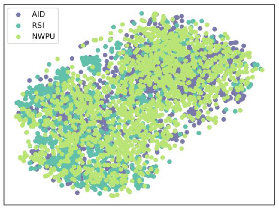
For continual learning across different datasets, we set the AID dataset as the first step of the scene classification task; the RSI-CB256 and NWPU-45 datasets were subsequently added in the second and third steps of the task, respectively. As can be seen in Figure 5, it is a challenging task to perform continual learning across different domain datasets. We split the labeled samples of three datasets into the labeled supervised training set, unlabeled contrastive learning, and testing set. In order to simulate the data accumulation, we kept all the data used in the previous step for the next step. Specifically, we randomly selected 5% labeled and 5% unlabeled samples from the AID dataset for the first step of model training, and 5% samples for testing. In the second step, we used all samples from the AID dataset in the previous step and supplemented the RSI dataset with 5% labeled samples and unlabeled samples for training, and 5% samples for testing. Similarly, the NWPU45 dataset was supplemented in the third step with 5% labeled samples and 5% unlabeled samples for training, and 5% samples for testing. We normalized the image size of each dataset to 256 × 256 and performed random image augmentation. The random augmentations strategy adopts resize, random crop, rotation and color jitter, etc.

In our experiments, pre-trained wideresent-50 [49] on ImageNet was used as the backbone to extract multilayer features for knowledge distillation. The MLP with three hidden layers is employed to project the features to the space where contrastive loss is computed. In the continual learning task across datasets, we used only annotated samples at the first step, and the size of the mini-batch was set to 24. And in the following two tasks, we set the mini-batch size to 16 for both the annotated and unannotated samples. The number of training epochs was set to 50 for each step task. To maintain the knowledge of the historical model, the learning rate was set to 6 × 10^-5. The Adam optimizer was applied with weight decay 1e-5. The temperature was set to 0.1 in the contrastive loss.

All experiments in this article were executed with Python 3.7, and Pytorch 1.6. The operation system is centos7.6, two NVIDIA Tesla 100 with 16 G memory for GPU acceleration, and other equipment includes Intel (R) Xeon (R) Gold 5118 CPU and 256 G RAM.

4.3. Evaluation Metrics

In order to test the accuracy performance of the proposed model and other continual learning methods, we introduced OA (overall accuracy), Kappa coefficient, and the confusion matrix to measure the scene prediction accuracy. We therefore displayed the mean and standard deviation of the OA for all results after five experiments.

In addition, to further illustrate the knowledge forgetting and knowledge transferring during continual learning in the model [50], we introduced average task accuracy (AT) and average task forgetting accuracy (ATF). We define $a_{i,j}$ as the overall accuracy of the model on task j after the model is trained on i-th task. Therefore, for the T-step continual learning task, the AT of the current step i can be expressed as the average overall accuracy of the j-th task from task 1 to task i. The higher average task accuracy shows that the model achieved better performance over a series of continual learning tasks. The formula can be expressed as

$$AT=\frac{1}{i}{\displaystyle \sum }_{j=1}^i{a}_{i,j}$$

(13)

The average task forgetting accuracy represents the forgetting level of the model on task j after training on task i. Typically, the model has a higher knowledge forgetting of the previous tasks during continual learning, when the ATF is higher. The ATF for current task i can be calculated as follows

$$ATF=\frac{1}{\mathrm{i}-1}{\displaystyle \sum }_{j=1}^{i-1}{f}_{i,j}$$

(14)

$$\mathrm{where} f_{k,j}=\underset{l\in \left\{1,\dots ,k-1\right\}}{max}\left(a_{l,j}\right)-a_{k,j},\forall j<K$$

where $\underset{l\in \left\{1,\dots ,k-1\right\}}{max}\left(a_{l,j}\right)$ represents the best overall accuracy achieved by the model for task j after training on the i-th task. $f_{i,j}$ is calculated to show how much knowledge has been forgotten about task j since the model trained on task i.

5. Results of Experiments

5.1. Ablation Study

5.1.1. Effect of Different Loss

To assess the contribution of different loss functions of our proposed method on forgetting prevention across three different datasets, we compared three different loss functions and performed several ablation experiments in this section. In the AID, RSI, and NWPU datasets, we randomly selected 5%, 5%, and 5% of the labeled samples for training, respectively. In addition, 5% of the samples without labels were trained with contrastive loss, and 5% of the samples were selected for testing. These ablation studies include (1) CE—the basic loss function for model training; (2) CE + Spatial loss—this combination is used to preserve the learned spatial knowledge of the historical model; (3) CE + Class loss—this combination is used to distill the high-level knowledge to the current model; (4) CE + Contra—this combination is used to obtain discriminative features; (5) CE + Spa + Class—this combination is used to distill the hidden and high-level knowledge to the current model; (6) CE + Spatial loss + Class loss + Contra loss—this combination adds contrastive learning to the previous loss function to enhance model feature representation further. The results of the ablation studies are demonstrated as follows.

As shown in

Table 1. Ablation study results for our continual learning method CCLnet on three-step tasks.

	CE	Spa	Class	Contra	Step1	Step2			Step3
					AID	AID	RSI	AID	RSI	NWPU
1	√				83.37	67.74	90.00	61.46	82.21	72.57
2	√	√			83.37	70.79	89.01	66.53	83.78	70.22
3	√		√		83.37	70.38	87.70	66.12	86.07	71.75
4	√			√	83.37	70.99	89.18	60.44	86.31	74.60
5	√	√	√		83.37	71.81	87.30	67.34	85.90	73.65
6	√	√	√	√	83.37	72.41	90.49	67.74	87.79	74.65

, satisfied accuracy was obtained for the method which used spatial loss, class loss and contrast loss simultaneously. It was found that using only cross-entropy causes the historical knowledge to be covered by the newly learned knowledge of the model. For this reason, the spatial loss and category loss introduced help the model preserve the knowledge learned from the historical datasets in the third step and alleviate the forgetting of knowledge effectively. In addition, combining the spatial and class losses produced better results in terms of knowledge retention in the latter two steps. This ensures that knowledge is transferred from the historical model to the new step model training. Eventually, contrastive loss is introduced to enhance the representativeness of the acquired features in the continual learning process, which leads to better performance in enabling the model to retain historical knowledge. The above experimental results indicate that our proposed method could lead to a favorable performance on continual scene classification tasks across different datasets.

5.1.2. Weights Effect

To further evaluate the effect of different loss functions, we divided the total loss function into two fractions, a knowledge learning module (KL) combined by CE + Contra, and a knowledge retaining (KR) module that combined by Spa + Class. We changed the weights of these two modules in the total loss function four times. The results are shown in

Table 2. The influence of different module weights on model accuracy.

Ratio (KL:KR)	Step1	Step2			Step3
	AID	AID	RSI	Average	AID	RSI	NWPU	Average
0.1:0.9	81.14	69.57	86.72	78.15	66.28	85.08	65.26	71.21
0.3:0.7	81.14	70.58	88.20	79.39	68.35	84.59	66.29	73.08
0.5:0.5	81.14	70.18	90.16	80.17	67.74	84.90	71.62	74.75
0.6:0.4	81.14	68.15	89.59	78.87	61.05	84.42	73.20	72.89
0.9:0.1	81.14	67.74	91.63	79.69	61.05	84.34	71.55	72.21

. In the table, we can see that the model retains historical knowledge effectively as the weight of the KR module increases, whereas it fails to learn new knowledge efficiently. In contrast, the model demonstrates a stronger tendency to learn new knowledge with increasing weight of the KL module. However, the average accuracy of the model over a series of tasks does not increase consistently with the weight of the KL or KR module. Therefore, to balance knowledge learning and retention, we set the ratio of the two modules to 0.5:0.5.

5.1.3. Average Accuracy and Average Forgetting

As shown in Figure 6, to assess the potential contribution of the different loss functions of the model on the new knowledge learning and the historical knowledge preserving during continual learning, we plot the average task accuracy curve and the average task forgetting curve for the different modules in the three step tasks. The red line indicates the accuracy curve applying CE loss, Spatial loss and Class loss and the Contrastive loss together. As can be seen from the figures, our approach enables new knowledge learning from the novel data while maintaining the historical knowledge. This means that the higher the average task accuracy curve in the left figure, the lower the average task forgetting accuracy curve in the right figure. Comparing with the combined spatial and class loss, incorporating contrastive loss further enhances the robustness of the features during continuous learning, leading to a better performance in alleviating catastrophic forgetting. Thus, our proposed loss modules are found to be effective for continual learning across datasets.

5.2. Comparison with Other Methods

In this section, we evaluate the performance of our proposed model and other representative continual learning methods across three different large-scale scene datasets. For example, Learning without Forgetting (LwF) [44], Synaptic Intelligence (SI) [51], Context-dependent-Gating (XdG) [52], EWC [15] and Online EWC [53] were used as comparison methods for comparison tests. For fair comparison, the same training and validation samples were selected for all methods for each experiment. For these methods, the detailed hyperparameters are set as follows: the λ parameter in LWF and EWC are set to 1 and 50, respectively, and the λ parameter and gamma in Online EWC are set to 50 and 1, respectively. The percentage of hidden units to gate in XDG is set to 0.8. The regularization strength c in SI is set to 0.1. The principles of these methods are explained as follows.

The EWC method employs sequential Bayesian estimation and proves second derivatives of parameters to measure the importance of these parameters for continual learning. For this reason, the EWC sets the parameter penalty terms for each step of the tasks in the continual learning process. However, maintaining multiple parameter penalty terms causes a huge computational overhead as the model is continually updated. Therefore, EWC-online keeps only the penalty for the most recent task parameters and then further alleviates the computational resource consumption. Similar to EWC, SI punishes the update of importance weights by measuring synaptic importance, and the synapses are built to accumulate information about sequential learning tasks, which allows new knowledge to be learnt quickly and avoids forgetting historical knowledge. The LWF method firstly uses knowledge distillation strategy to retain knowledge of historical tasks to continual learning tasks. It uses the output of the old model to instruct the parameters of the new task model to be updated. Therefore, it performs well on both old and novel tasks and alleviates catastrophic forgetting of the model effectively. Finally, XdG employs a random assignment strategy for each task to decide which units of the model will be used for every task. Hence, it is suitable for incremental learning.

Compared with these methods mentioned above, our proposed method achieves optimal performance among a series of scene dataset classification tasks. As shown in

Table 3. Overall accuracy of comparison methods on three-step continual scene classification tasks.

Method	Step1	Step2		Step3
	AID	AID	RSC-256	AID	RSC-256	NWPU-45
EWC	37.12	22.11	65.66	24.75	32.46	29.40
Online-ewc	32.25	11.56	64.02	8.32	30.82	27.75
LWF	30.22	26.77	68.93	30.02	61.64	31.56
XDG	39.35	28.19	78.36	32.45	43.44	34.86
SI	31.85	11.16	65.57	11.16	21.15	30.35
Fine-tuning	80.43	67.51	83.64	62.55	81.26	70.24
Ours	83.37	72.41	90.49	67.74	87.79	74.65

, the overall accuracy of our method fine-tuning, and other classic continual learning methods are displayed. For the three continually updated scene datasets, the above baseline continual learning approaches perform the three step continual learning tasks well; in particular, the LWF and XDG avoided catastrophic forgetting effectively. However, these methods are insufficient for acquiring new knowledge quickly through exploiting new datasets. For example, the LWF method obtained 68.93% accuracy on the new RCS dataset in the second step task, whereas only 31.56% overall accuracy was obtained when the new NWPU dataset was added in the third step task. Our model produced the top accuracy in the three-step continual learning process for each remote scene dataset. In the first step task of the AID dataset classification, the overall accuracy of our model improved at least 53.15% compared with other classical methods. For the second step classification task on the AID and RSC datasets, our method improved by at least 44.22% and 12.13%, respectively. For the three datasets in the third step, our method still shows at least 35.2%, 26.15%, and 28.18% improvement, respectively. Therefore, our proposed model performs better in learning new knowledge.

In addition, to provide a detailed description of the classification accuracy changes for each category during the continual learning process, as shown in

Table 4. Classification accuracy of partially scenes during three-step continual learning tasks.

	Step1	Step2		Step3
Category	AID	AID	RSC-256	AID	RSC-256	NWPU-45
0	77.78	100.0	77.78	83.33	64.71	80.0
1	73.33	100.0	66.67	53.33	100.0	88.57
2	100.0	78.57	90.91	63.64	57.14	91.43
3	100.0	74.07	50.0	50.0	77.78	80.0
4	94.44	81.4	88.89	61.11	83.72	57.14
5	69.23	69.57	69.23	53.85	86.96	71.43
6	75.0	90.0	41.67	75.0	88.0	82.86
7	94.12	68.18	76.47	100.0	63.64	48.57
8	85.0	100.0	70.0	75.0	100.0	91.43
9	60.0	100.0	73.33	33.33	92.59	88.57
10	100.0	43.75	61.11	66.67	43.75	51.43
11	100.0	88.89	91.67	91.67	68.52	74.29
12	73.68	95.38	73.68	63.16	98.46	68.57
13	78.57	98.15	85.71	50.0	98.15	77.14
14	92.86	90.62	71.43	85.71	62.5	57.14
OA	84.78	76.47	91.80	70.38	86.72	71.93
K	0.84	0.76	0.92	0.70	0.86	0.71

, we present the classification overall accuracy and Kappa coefficient of the individual categories for the three datasets. We only present the first 15 categories for each dataset, due to the space limitation. In the aided dataset, classes 2, 3, 10 and 11, whose classification accuracy was 100% in the first step, suffered different levels of forgetting to the later steps. Especially for the class 2, class 3 and class 10, there is a significant forgetting during the three steps tasks. With the addition of following datasets, the model better obtained representative knowledge from the novel data sets. It is important for the model to recognize new categories precisely. For example, five categories of the RSI dataset with over 90% classification accuracy existed in the third stage, and two categories in the NWPU dataset.

5.3. Class Incremental Learning

In this section, we performed several comparison experiments on cross-domain datasets. To evaluate the incremental learning ability of our model within the same dataset, we split each dataset into 10 sections to simulate continual learning in longer data stream. For example, we provided 6, 6 and 5 new scenes for each of the first three steps of the NWPU dataset, and then supplemented each step with 4 new scene categories. We kept the same experimental settings as the cross-domain continuous learning task, including sample size and hyperparameter settings.

Table 5. Overall accuracy of class incremental learning on each of the three datasets.

Dataset	Step1	Step2	Step3	Step4	Step5	Step6	Step7	Step8	Step9	Step10
AID	100	99.43	95.13	92.59	87.71	87.20	89.04	89.34	86.13	86.21
RSI	99.47	97.23	96.08	93.97	93.27	87.06	87.14	87.65	86.65	89.63
NWPU	94.28	93.81	92.26	88.57	86.97	82.17	80.08	81.31	80.62	78.66

presents the accuracy evaluation of class incremental learning on different datasets. We can see that the early steps of the model obtained a high accuracy. However, with the supplementation of new scene categories, the overall accuracy of the model decreases gradually for all learned scene categories. Compared with the AID dataset and RSI dataset, the NWPU dataset has a 15.62% reduction in accuracy from the first to the last step. Due to the large intra-class diversity and inter-class similarity, the complex NWPU scene dataset causes the model to be more likely to be confused during continuous learning.

5.4. Confusion Matrix

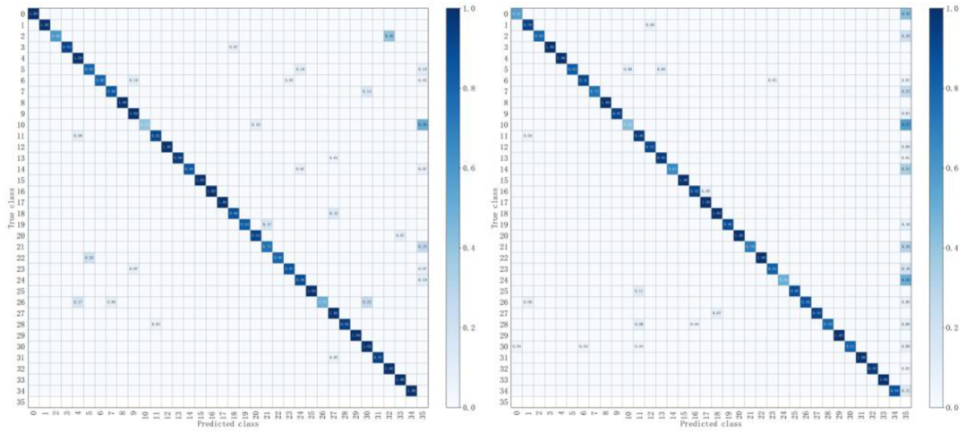
We demonstrate the confusion matrix of classification results for each method on different steps of the scene classification task in detail. Through the confusion matrix, the category accuracy and misclassification can be seen clearly. The i-th row and j-th column represent the classification accuracy of the i-th class of scenes predicted as the j-th class. Since the model suffers from classification confusion across datasets during continual learning, we introduced additional categories on the second and third step tasks to represent the results of classifying the current dataset into the images of other datasets.

In Figure 7, Figure 8 and Figure 9, we display the confusion matrices for the three-step classification results of our proposed method. Our method accurately recognized most of the scene images. From these figures, we can see that there are fewer misclassified scenes in the AID dataset for the first step. With the added RSI and NWPU datasets, the number of misclassifications in the AID dataset gradually increased. Specifically, all categories obtained comparable accuracy at the first step. The bare land (class 1), beach (class 3), desert (class 9), meadow (class 13), etc. can easily be categorized into another dataset. This is because these similar scenes are shared across these different scene datasets. Similarly, for the RSI dataset, several scenes could still be misclassified into other datasets easily, especially the scene imagery of dam (class 9) and parking lot (class 21). As for the large-scale NWPU dataset, due to the significant inter-class similarity and intra-class variation, the misclassification not only occurred within the dataset, but also across different domain datasets. Nevertheless, comparing the confusion matrix of model classification results at different stages, our method provides favorable results in the continual learning process across different datasets. This demonstrates that our method obtains valuable information quickly from new datasets without compromising the performance of the model on historical data.

5.5. Visualization Results

The critical importance for the scene classification task is that the model focuses accurately on the important regions of the scene. Therefore, we used a Score-cam attention heatmap to evaluate whether the model focuses on the representative area of the image when making decisions. The wideresnet50 was employed as the backbone of our model to extract features. Hence, the attention heatmap can be used to discriminate the representativeness of the features at different levels of the backbone network. The visualizations of these features are used to further interpret the model on scene classification tasks. In the heatmap, the darker color indicates the area which receives more attention from the model.

In Figure 10, the visualization results of the model based on the three datasets AID, RSI and NWPU45 are illustrated. The heatmap of low-level features shows that the model pays more attention to the edges of objects in the scene images. The model prefers to understand complex scene images from the obtained abstract high-level information as the number of model layers becomes deeper. As shown in Figure 10a, the visually interpretable maps of airport and viaduct on the AID dataset prove that the attention of the shallow model is mostly positioned on the local area of the scene image, such as a separate airplane in the airport and an individual storage tank, and focuses on characteristics of edges and corners. As for complicated scenes such as parks, the model focuses on more local details of the whole image due to the complexity of the internal object types. The saliency areas of the high-level feature heat map show that the model is more concerned with global and abstract information. Therefore, the representative features can be used to discriminate complex scene images.

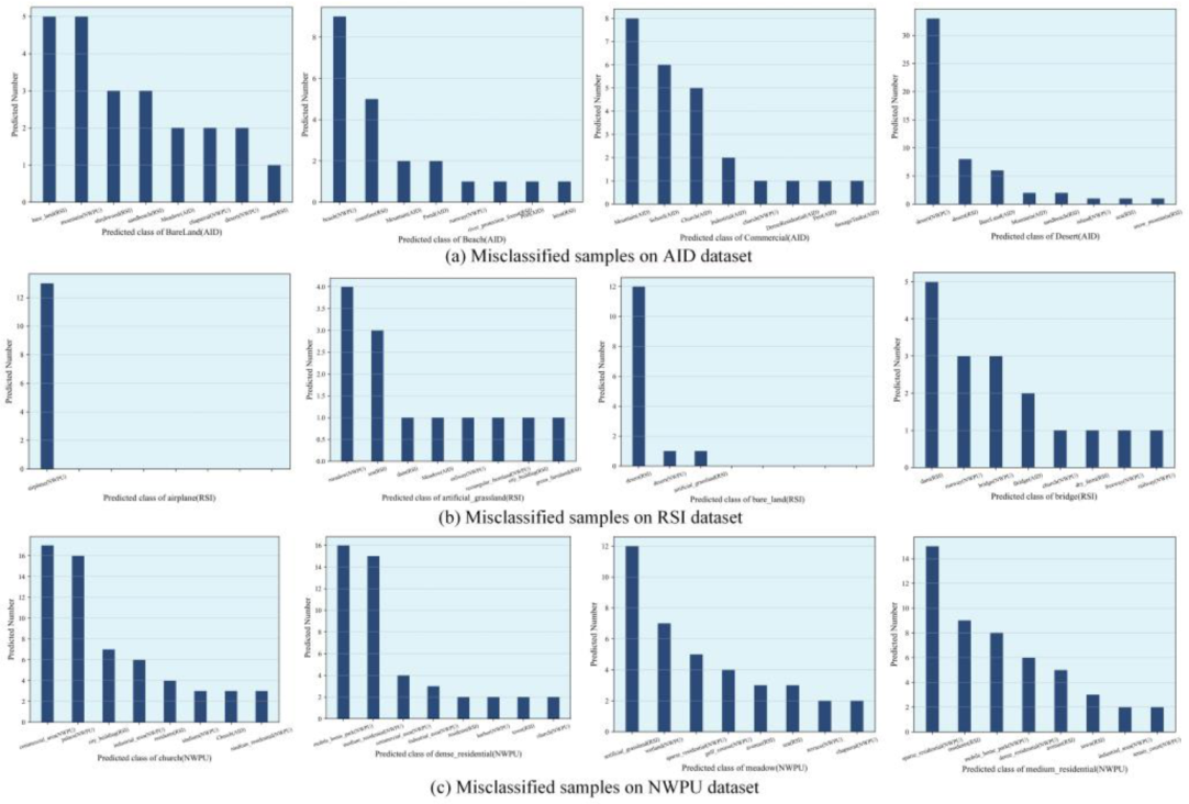
From Figure 11 and Figure 12, we can see that several misclassified scene images and corresponding misclassified images on AID, RSI and NWPU datasets, respectively. Similar to previous confusion matrixes, seen in the result shown in Figure 12, the misclassified scene images in the AID and RSI datasets are mostly occurring in the common class. Instead, as a large-scale dataset, the misclassification in the NWPU dataset often occurs inside the dataset. This is because more intense inter-class similarity problems are encountered across different datasets during continual learning, for example, the beach, the bare land between the AID dataset and RSI dataset, and the airplane, meadow and residential between NWPU and RSI dataset.

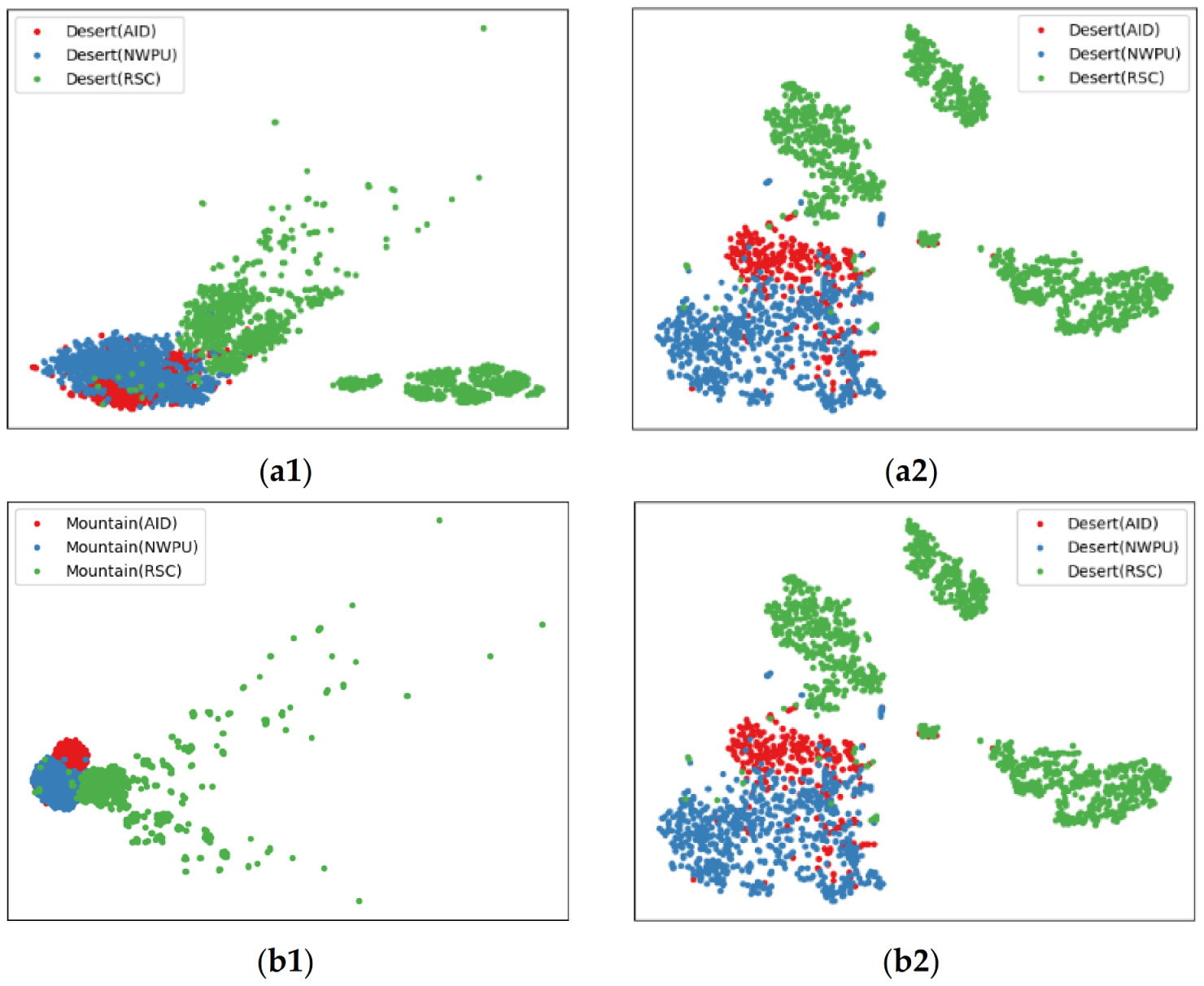
For the scenes belonging to the same class contained in all three datasets, especially for the common desert, mountain and other categories, misclassification occurs during the continual learning process, which results from color and texture similarity. Furthermore, to evaluate the feature representation of our proposed method in the continual learning, we applied the t-SNE algorithm [54] for visualizing obtained high dimensional features to low dimensional space, which mapped the probability distribution of high dimensional features and low dimensional features. We obtained the features of the same category of scene images on three datasets. The t-SNE is applied to reducing the high dimensional features to a 2-D space. As can be seen from Figure 13, the fourth layer features of the desert and mountain scenes are so close in the feature space that the model cannot recognize them accurately, while the deeper features of the images increase further in the feature space with continuous learning, and the model can better discriminate such similar scene images. As a result, our model can effectively alleviate the within-class diversity and inter-class similarity problems across different datasets and perform better in continual scene classification tasks.

6. Conclusions

In recent years, many scene classification methods have been developed to address the problem of scene classification in the remote sensing field. Faced with continually updated remote sensing data, the model usually tends to perform better on new data rather than on historical data, i.e., there is a catastrophic forgetting problem. In this paper, we propose a continual contrastive learning network (CCLNet) for scene classification with an updating dataset. Our proposed model uses wideresnet50 as the backbone network and designs spatial loss, category loss and contrast loss for model training. At first, we used cross-entropy for the initial model training. Then, we retained the knowledge learned in the previous step task into the current model through spatial and class loss. Finally, we further enhanced the extracted features to improve the classification performance of the model during the continual learning of the model by using contrastive loss. Compared with other continual learning models, extensive experiments prove that our proposed model outperforms on different datasets. In future, we will explore remote sensing scene classification tasks under more challenging conditions, such as combining few-shot learning to overcome unknown sample prediction problems for open-set identification.

References

1. Huang, X.; Han, X.; Ma, S.; Lin, T.; Gong, J. Monitoring ecosystem service change in the City of Shenzhen by the use of high-resolution remotely sensed imagery and deep learning. L. Degrad. Dev. 2019, 30, 1490–1501. [Google Scholar] [CrossRef]
2. Ghazouani, F.; Farah, I.R.; Solaiman, B. A Multi-Level Semantic Scene Interpretation Strategy for Change Interpretation in Remote Sensing Imagery. IEEE Trans. Geosci. Remote Sens. 2019, 57, 8775–8795. [Google Scholar] [CrossRef]
3. Cheng, G.; Guo, L.; Zhao, T.; Han, J.; Li, H.; Fang, J. Automatic landslide detection from remote-sensing imagery using a scene classification method based on boVW and pLSA. Int. J. Remote Sens. 2013, 34, 45–59. [Google Scholar] [CrossRef]
4. Li, Y.; Zhang, Y.; Huang, X.; Yuille, A.L. Deep networks under scene-level supervision for multi-class geospatial object detection from remote sensing images. ISPRS J. Photogramm. Remote Sens. 2018, 146, 182–196. [Google Scholar] [CrossRef]
5. Chen, C.; Gong, W.; Chen, Y.; Li, W. Object detection in remote sensing images based on a scene-contextual feature pyramid network. Remote Sens. 2019, 11, 339. [Google Scholar] [CrossRef] [Green Version]
6. de Lima, R.P.; Marfurt, K. Convolutional neural network for remote-sensing scene classification: Transfer learning analysis. Remote Sens. 2020, 12, 86. [Google Scholar] [CrossRef] [Green Version]
7. Li, W.; Wang, Z.; Wang, Y.; Wu, J.; Wang, J.; Jia, Y.; Gui, G. Classification of high-spatial-resolution remote sensing scenes method using transfer learning and deep convolutional neural network. IEEE J. Sel. Top. Appl. Earth Obs. Remote Sens. 2020, 13, 1986–1995. [Google Scholar] [CrossRef]
8. Song, S.; Yu, H.; Miao, Z.; Zhang, Q.; Lin, Y.; Wang, S. Domain adaptation for convolutional neural networks-based remote sensing scene classification. IEEE Geosci. Remote Sens. Lett. 2019, 16, 1324–1328. [Google Scholar] [CrossRef]
9. De Lange, M.; Aljundi, R.; Masana, M.; Parisot, S.; Jia, X.; Leonardis, A.; Slabaugh, G.; Tuytelaars, T. A continual learning survey: Defying forgetting in classification tasks. IEEE Trans. Pattern Anal. Mach. Intell. 2021, 44, 3366–3385. [Google Scholar]
10. Rebuffi, S.-A.; Kolesnikov, A.; Sperl, G.; Lampert, C.H. iCaRL: Incremental Classifier and Representation Learning Sylvestre-Alvise. In Proceedings of the Proceedings of the IEEE Conference on Computer Vision and Pattern Recognition, Honolulu, HI, USA, 21–26 July 2017; pp. 2001–2010.
11. Kamra, N.; Gupta, U.; Liu, Y. Deep Generative Dual Memory Network for Continual Learning. arXiv 2017, arXiv:1710.10368. [Google Scholar]
12. Rostami, M.; Kolouri, S.; Pilly, P.; McClelland, J. Generative continual concept learning. In Proceedings of the AAAI Conference on Artificial Intelligence, New York, NY, USA, 7–12 February 2020; Volume 34, pp. 5545–5552. [Google Scholar]
13. Shin, H.; Lee, J.K.; Kim, J.; Kim, J. Continual learning with deep generative replay. Adv. Neural Inf. Process. Syst. 2017, 30. [Google Scholar]
14. Verma, V.K.; Liang, K.J.; Mehta, N.; Rai, P.; Carin, L. Efficient feature transformations for discriminative and generative continual learning. In Proceedings of the IEEE/CVF Conference on Computer Vision and Pattern Recognition, Virtual, 19–25 June 2021; pp. 13865–13875. [Google Scholar]
15. James, K.; Razvan, P.; Neil, R.; Joel, V.; Guillaume, D.; Rusu, A.A.; Kieran, M.; John, Q.; Tiago, R.; Agnieszka, G.-B.; et al. Overcoming catastrophic forgetting in neural networks. Proc. Natl. Acad. Sci. USA 2017, 114, 3521–3526. [Google Scholar] [CrossRef] [Green Version]
16. Aljundi, R.; Babiloni, F.; Elhoseiny, M. Memory Aware Synapses: Learning what ( not ) to forget. In Proceedings of the European Conference on Computer Vision (ECCV), Munich, Germany, 8–14 September 2018; pp. 139–154. [Google Scholar]
17. Parisi, G.I.; Kemker, R.; Part, J.L.; Kanan, C.; Wermter, S. Continual lifelong learning with neural networks: A review. Neural Networks 2019, 113, 54–71. [Google Scholar] [CrossRef]
18. Yoon, J.; Yang, E.; Lee, J.; Hwang, S.J. Lifelong Learning with Dynamically Expandable Networks. arXiv 2017, arXiv:1708.01547. [Google Scholar]
19. Rusu, A.A.; Rabinowitz, N.C.; Desjardins, G.; Soyer, H.; Kirkpatrick, J.; Kavukcuoglu, K.; Pascanu, R.; Hadsell, R. Progressive Neural Networks. arXiv 2016, arXiv:1606.04671. [Google Scholar]
20. Fernando, C.; Banarse, D.; Blundell, C.; Zwols, Y.; Ha, D.; Rusu, A.A.; Pritzel, A.; Wierstra, D. Pathnet: Evolution channels gradient descent in super neural networks. arXiv 2017, arXiv:1701.08734. [Google Scholar]
21. Mallya, A.; Lazebnik, S. PackNet: Adding Multiple Tasks to a Single Network by Iterative Pruning. In Proceedings of the IEEE Conference on Computer Vision and Pattern Recognition (CVPR), Salt Lake City, UT, USA, 18–22 June 2018; pp. 7765–7773. [Google Scholar]
22. Lee, J. Co2L: Contrastive Continual Learning. arXiv 2021, arXiv:2106.14413. [Google Scholar]
23. Zhao, Z.; Luo, Z.; Li, J.; Chen, C.; Piao, Y. When self-supervised learning meets scene classification: Remote sensing scene classification based on a multitask learning framework. Remote Sens. 2020, 12, 3276. [Google Scholar] [CrossRef]
24. Tao, C.; Qi, J.; Lu, W.; Wang, H.; Li, H. Remote Sensing Image Scene Classification with Self-Supervised Paradigm Under Limited Labeled Samples. IEEE Geosci. Remote Sens. Lett. 2022, 19, 1–5. [Google Scholar] [CrossRef]
25. Stojnić, V.; Risojević, V. Self-Supervised Learning of Remote Sensing Scene Representations Using Contrastive Multiview Coding. In Proceedings of the IEEE/CVF Conference on Computer Vision and Pattern Recognition (CVPR) Workshops, Nashville, TN, USA, 19–25 June 2021; pp. 1182–1191. [Google Scholar]
26. Zou, Q.; Ni, L.; Zhang, T.; Wang, Q. Remote Sensing Scene Classification. IEEE Trans. Geosci. Remote Sens. Lett. 2015, 12, 2321–2325. [Google Scholar] [CrossRef]
27. Marmanis, D.; Datcu, M.; Esch, T.; Stilla, U. Using ImageNet Pretrained Networks. IEEE Trans. Geosci. Remote Sens. Lett. 2016, 13, 105–109. [Google Scholar] [CrossRef] [Green Version]
28. Hu, F.; Xia, G.-S.; Wang, Z.; Huang, X.; Zhang, L.; Sun, H. Unsupervised Feature Learning Via Spectral Clustering of Multidimensional Patches for Remotely Sensed Scene Classification. IEEE J. Sel. Top. Appl. Earth Obs. Remote Sens. 2015, 8, 2015–2030. [Google Scholar] [CrossRef]
29. Chaib, S.; Liu, H.; Gu, Y.; Yao, H. Deep Feature Fusion for VHR Remote Sensing Scene Classification. IEEE Trans. Geosci. Remote Sens. 2017, 55, 4775–4784. [Google Scholar] [CrossRef]
30. He, K.; Fan, H.; Wu, Y.; Xie, S.; Girshick, R. Momentum Contrast for Unsupervised Visual Representation Learning. In Proceedings of the 2020 IEEE/CVF Conference on Computer Vision and Pattern Recognition (CVPR), Seattle, WA, USA, 13–19 June 2020; pp. 9726–9735. [Google Scholar] [CrossRef]
31. Chen, T.; Kornblith, S.; Norouzi, M.; Hinton, G. A simple framework for contrastive learning of visual representations. In Proceedings of the 37th International Conference on Machine Learning, PMLR, Virtual, 13–18 July 2020; pp. 1597–1607. [Google Scholar]
32. Chen, T.; Kornblith, S.; Swersky, K.; Norouzi, M.; Hinton, G. Big Self-Supervised Models are Strong Semi-Supervised Learners. Adv. Neural Inf. Process. Syst. 2020, 33, 22243–22255. [Google Scholar]
33. Caron, M.; Misra, I.; Mairal, J.; Goyal, P.; Bojanowski, P.; Joulin, A. Unsupervised Learning of Visual Features by Contrasting Cluster Assignments. Adv. Neural Inf. Process. Syst. 2020, 33, 9912–9924. [Google Scholar]
34. Grill, J.-B.; Strub, F.; Altché, F.; Tallec, C.; Richemond, P.; Buchatskaya, E.; Doersch, C.; Avila Pires, B.; Guo, Z.; Gheshlaghi Azar, M.; et al. Bootstrap Your Own Latent—A New Approach to Self-Supervised Learning. Adv. Neural Inf. Process. Syst. 2020, 33, 21271–21284. [Google Scholar]
35. Chen, X.; Ai, F. Exploring Simple Siamese Representation Learning. In Proceedings of the IEEE/CVF Conference on Computer Vision and Pattern Recognition (CVPR), Virtual, 19–25 June 2021; pp. 15750–15758. [Google Scholar]
36. Gomez, P.; Meoni, G. MSMatch: Semisupervised Multispectral Scene Classification with Few Labels. IEEE J. Sel. Top. Appl. Earth Obs. Remote Sens. 2021, 14, 11643–11654. [Google Scholar] [CrossRef]
37. Li, X.; Shi, D.; Diao, X.; Xu, H. SCL-MLNet: Boosting Few-Shot Remote Sensing Scene Classification via Self-Supervised Contrastive Learning. IEEE Trans. Geosci. Remote Sens. 2022, 60, 1–12. [Google Scholar] [CrossRef]
38. Huang, H.; Mou, Z.; Li, Y.; Li, Q.; Chen, J.; Li, H. Spatial-Temporal Invariant Contrastive Learning for Remote Sensing Scene Classification. IEEE Geosci. Remote Sens. Lett. 2022, 19, 1–5. [Google Scholar] [CrossRef]
39. Hinton, G.; Vinyals, O.; Dean, J. Distilling the knowledge in a neural network. arXiv 2015, arXiv:1503.02531. [Google Scholar]
40. Müller, R.; Kornblith, S.; Hinton, G. When does label smoothing help? Adv. Neural Inf. Process. Syst. 2019, 32. [Google Scholar]
41. Romero, A.; Ballas, N.; Kahou, S.E.; Chassang, A.; Gatta, C.; Bengio, Y. FitNets: Hints for thin deep nets. Proc. ICLR 2015, 1–13. [Google Scholar]
42. Zagoruyko, S.; Komodakis, N. Paying more attention to attention: Improving the performance of convolutional neural networks via attention transfer. In Proceedings of the 5th International Conference on Learning Representations, Toulon, France, 24–26 April 2017; pp. 1–13. [Google Scholar]
43. Ji, M.; Heo, B.; Park, S. Show, Attend and Distill: Knowledge Distillation via Attention-based Feature Matching. Proc. AAAI Conf. Artif. Intell. 2021, 35, 7945–7952. [Google Scholar] [CrossRef]
44. Li, Z.; Hoiem, D. Learning without Forgetting. IEEE Trans. Pattern Anal. Mach. Intell. 2018, 40, 2935–2947. [Google Scholar] [CrossRef] [Green Version]
45. Castro, F.M.; Mar, M.J.; Schmid, C. End-to-End Incremental Learning Francisco. Proc. Eur. Conf. Comput. Vis. 2018, 16–18. [Google Scholar]
46. Wu, Y.; Chen, Y.; Wang, L.; Ye, Y.; Liu, Z.; Guo, Y.; Fu, Y. Large scale incremental learning. In Proceedings of the 2019 IEEE/CVF Conference on Computer Vision and Pattern Recognition (CVPR), Long Beach, CA, USA, 15–20 June 2019; pp. 374–382. [Google Scholar] [CrossRef] [Green Version]
47. Xia, G.S.; Hu, J.; Hu, F.; Shi, B.; Zhang, L. AID: A Benchmark Data Set for Performance Evaluation of Aerial Scene Classification. IEEE Trans. Geosci. Remote Sens. 2017, 55, 3965–3981. [Google Scholar] [CrossRef] [Green Version]
48. Cheng, G.; Han, J.; Lu, X. Remote Sensing Image Scene Classification: Benchmark and State of the Art. Proc. IEEE 2017, 105, 1865–1883. [Google Scholar] [CrossRef] [Green Version]
49. Zagoruyko, S.; Komodakis, N. Wide Residual Networks. In Proceedings of the British Machine Vision Conference (BMVC), York, UK, 19–22 September 2016; pp. 87.1–87.12. [Google Scholar] [CrossRef] [Green Version]
50. Mai, Z.; Li, R.; Jeong, J.; Quispe, D.; Kim, H.; Sanner, S. Online continual learning in image classification: An empirical survey. Neurocomputing 2022, 469, 28–51. [Google Scholar] [CrossRef]
51. Zenke, F.; Poole, B.; Ganguli, S. Continual Learning Through Synaptic Intelligence. In Proceedings of the International Conference on Machine Learning, Sydney, Australia, 6–11 August 2017; pp. 3987–3995. [Google Scholar]
52. Masse, N.Y.; Grant, G.D.; Freedman, D.J. Alleviating catastrophic forgetting using context- dependent gating and synaptic stabilization. Proc. Natl. Acad. Sci. USA 2018, 115, E10467–E10475. [Google Scholar] [CrossRef] [Green Version]
53. Huszár, F. Note on the quadratic penalties in elastic weight consolidation. Proc. Natl. Acad. Sci. USA 2018, 115, E2496–E2497. [Google Scholar] [CrossRef]
54. Laurens, V.D.M.; Hinton, G. Visualizing Data using t-SNE. J. Mach. Learn. Res. 2008, 9, 2579–2605. [Google Scholar]
Figure 1. Overview of our proposed framework.
Remotesensing 14 05105 g001
Figure 2. Several scene image samples in AID dataset.
Remotesensing 14 05105 g002
Figure 3. Several scene image samples in NWPU dataset.
Remotesensing 14 05105 g003
Figure 4. Several scene image samples on RSI dataset.
Remotesensing 14 05105 g004
Figure 5. 2-D scatter plots for three scenes datasets in feature space, which was generated with the t-SNE algorithm.
Remotesensing 14 05105 g005
Figure 6. Average task accuracy curve (a) and average task forgetting accuracy curve (b) for different combinations of loss function on three-step continual learning tasks.
Remotesensing 14 05105 g006
Figure 7. From left to right, the confusion matrix for each of the three steps on the AID dataset.
Remotesensing 14 05105 g007
Figure 8. The confusion matrices of second and third step on RSI dataset.
Remotesensing 14 05105 g008
Figure 9. The confusion matrix of third step task on NWPU dataset.
Remotesensing 14 05105 g009
Figure 10. Heat map visualization results of the model on different datasets in the third step. (ac) represent the results on the AID, RSI, and NWPU datasets, respectively. The first row of each subplot represents the original image, the second row represents the fourth layer attention map of the backbone network, and the third row represents the fully connected layer attention map of the model.
Remotesensing 14 05105 g010
Figure 11. Misclassified samples of AID, RSI and NWPU datasets on third step task. (a) represents the misclassified category in the AID dataset, (b) represent the misclassified scenes in the RSI dataset, (c) indicates the misclassified category in NWPU datasest.
Remotesensing 14 05105 g011
Figure 12. Histograms of misclassified samples among the three datasets. (a) indicates the statistic results of misclassified scenes on the AID dataset; (b) indicates the statistic results of misclassified scenes on the RSI dataset; (c) indicates the statistical results of misclassified scenes on the NWPU dataset.
Remotesensing 14 05105 g012
Figure 13. 2-D scatter plots for desert and mountain scenes feature which generated with t-SNE algorithm among the three datasets. (a1,a2) indicates the visualization result of desert features (b1,b2) represents the visualization result of mountain features. The first column represents the visualization results of 131,072-dimensional features acquired in the fourth layer of backbone, the second column indicates the visualization results of 128-dimensional features acquired at fourth layer and fully connected layer.
Remotesensing 14 05105 g013