Assessment of Sentinel-2-MSI Atmospheric Correction Processors and In Situ Spectrometry Waters Quality Algorithms

Abstract

The validation of algorithms developed from in situ reflectance to estimate water quality variables has the challenge of atmospheric correction (AC) when applied to satellite images. Estimating water quality variables from satellite images requires an accurate estimation of remote sensing reflectances (Rrs) which vary according to the AC applied. Validation processes for both Rrs and water quality algorithms were carried out, relating the in situ Rrs (convoluted to Sentinel-2-MSI spectral response function) with the satellite Rrs coming from different ACs (C2RCC, C2X, C2XC, and Polymer), and also relating the in situ water quality variable data with estimated water quality variable values, applying the water quality algorithms to the Rrs obtained for each AC. Regarding the Rrs validation results, the best ACs tested in this work were C2XC and Polymer. Regarding the water quality algorithm validation, the best results were also obtained using C2XC and Polymer Rrs. The results demonstrate the usefulness of the water quality algorithms developed from in situ reflectances since they are not specific to an AC and can be used with any processor.

1. Introduction

Remote sensing offers substantial advantages over traditional monitoring methods, mainly because of the synoptic coverage and temporal consistency of the data, and it has the potential to provide crucial information on inland and near-coastal transitional waters [1]. For this reason, remote sensing is an essential tool for the study and monitoring of inland water bodies, often characterized by Case 2 waters (optically complex waters), especially when it comes to studying key variables to determine water quality along a reservoir’s longitudinal profile. Because of this importance, many works develop algorithms based on in situ reflectance for various reasons: the validation of a previously published reflectance band-ratio algorithm [2] to use historical and unpublished data [3], obtaining algorithms in advance of the sensor’s activity [3,4], to develop cross-instrument algorithms to facilitate the spatial and temporal comparability of overlapping missions [5], and to achieve a wider range of data [6].

However, when the algorithms developed from in situ reflectances are applied to satellite imagery, their performance also depends on the errors in the water reflectance retrieval after the atmospheric correction. Estimating water quality variables from satellite images requires an accurate estimation of water-leaving radiance, but the radiation measured by the sensors has another important contributor, the atmosphere, consisting of atmospheric gases and aerosols, which account for at least 90% of the signal measured by the satellite sensor [7,8]. Therefore, the atmospheric correction (AC) procedure is an important step to subtract the atmospheric contribution (scattering effects of aerosols, water vapor, etc. …) and sun glint (sunlight reflecting off the water surface at the same angle as the sensor) from the signal at the top of the atmosphere (TOA) [9].

With regard to Case 2 waters, the algorithms designed to perform the AC of land surfaces are not directly applicable to an aquatic surface because it is darker, and the air-water interface is not Lambertian [9]. Nevertheless, a significant correlation has been demonstrated between the reflectance obtained by the Sen2Cor processor, developed for the land surface study of Sentinel-2 (S2-MSI) imagery, and the in situ reflectance for hypertrophic waters [10,11]. In addition, Case 2 waters are much more complex than oceanic waters (Case 1 waters) because of their optically active constituents (OAC) as they contain a higher presence of phytoplankton, dissolved organic matter, and tripton, therefore requiring a specific AC. Each OAC has a very different effect on the reflective spectrum; the suspended matter increases the reflectance in the green, red, and NIR bands, while the CDOM (chromophoric dissolved organic matter) increases the absorption (reducing the reflectance) in the blue bands [12]. Consequently, they strongly condition the water spectrum because the percentage contribution of water reflectance in TOA varies depending on the predominance of suspended sediment or CDOM in the water [13]. Therefore, due to the higher complexity of inland waters in the NIR, the ACs designed for Case 1 waters are generally not applicable to Case 2 waters. This indicates that different ACs may be required for waters of different OAC compositions, depending on the part of the spectrum used to perform the atmospheric correction.

To respond to this challenge, from before the launch of the S2-MSI mission satellites and up to the present day, different types of ACs are being developed for different Case 2 water types, even though the mission objective is soil and vegetation study. The great interest in S2-MSI is due to the fact that its usefulness has been proven for inland water study, thanks to the inclusion of new bands at the red edge (boundary of the red and infrared spectral regions), their radiometric quality, and their high spatial resolution [14]. A lot of the ACs to obtain water reflectance from S2-MSI images have been developed by the European Space Agency (ESA) and are provided in the freely available SNAP (SeNtinel Application Platform) program toolkit. Initially, there was only the C2RCC (Case 2 Regional Coast Colour) processor, which was developed from the original Case 2 regional processor [15] and adapted to different multi and hyperspectral sensors (e.g., S2-MSI and Sentinel-3-OLCI). Currently, a set of three different neural networks (NN) are available for S2-MSI imagery, trained with different databases to perform the AC on different water types and named here as C2-Nets: C2RCC, C2X (Case2eXtreme), and C2X-COMPLEX (C2XC). Another algorithm is Polymer; with its generic approach, it has been applied to many sensors, including S2-MSI and S3-OLCI. The Polymer approach is a physical model based on a spectral optimization method called spectral matching which is aimed at recovering the radiation scattered and absorbed by water from the measured signal by satellite sensors in the visible spectrum [16,17]. One of the strengths of this algorithm is the ability to recover water radiation in the presence of sun glint, achieving a spatial coverage higher than other products. With Polymer and the C2-Nets, the best S2-MSI radiation validation results have been obtained, as published in previous studies for Case 2 waters, such as those carried out by Ansper and Alikas [18], Pereira-Sandoval et al. [12], Uudeberg et al. [19], Warren et al. [20], and Bui et al. [21].

Once the AC has been applied and the water leaving reflectance has been obtained, the next step is obtaining the retrieval algorithms to estimate the different bio-optical variables, either empirically or analytically. In this sense, the objective is always to obtain a general algorithm, but the great difference in waters with respect to their OAC greatly conditions the results, as in the case of the AC step. The problem with validating the AC algorithms lies in the need to measure the in situ reflectance coinciding with the satellite pass, having a cloud-free image, good wind conditions, and all the involved costs of performing the sampling. Thus, an alternative is to use in situ reflectance data from previous studies, even if they are not coincidental with the satellite pass or even before its launch, to develop the algorithms, which will be validated with different ACs applications and with in situ water quality measurements. In this way, the database can be much larger, giving greater consistency and the water quality retrieval algorithms obtained more robust.

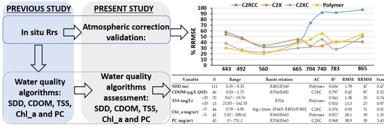
In this way, the work elaborated and published by Sòria-Perpinyà et al. [6] (previous study) was developed, in which five retrieval algorithms using in situ spectrometry were implemented to estimate five water quality variables such as transparency (Secchi disk depth, SDD), total suspended solids (TSS), CDOM, chlorophyll concentration (Chl_a), and phycocyanin concentration (PC), for both S2-MSI and S3-OLCI. This provides us with accurate and robust algorithms developed with in situ reflectance and not specific to a given AC. However, the obtained in situ spectrometry water quality algorithms need to be assessed using different ACs water reflectance because the application with reflectances obtained after an AC process may lead to unexpected results. It is necessary because, in the case of water, the validation of the reflectance resulting from the atmospheric correction is very difficult (the error could be of the same order as the surface reflectance itself). That is why the idea of validating the final products on water quality is the right approach, in particular for water. After all, the interest is not so much in the reflectance of the water itself but in its properties.

Therefore, the article is the second part of a previous study to complete the applicability step that was missing in other works, where only in situ reflectances were used to develop algorithms. With the aim of carrying out this applicability of the algorithms, the validation process has been conducted to test the best of those algorithms when we apply them to satellite S2-MSI imagery after the correction of atmospheric and sun specular effects.

2. Materials and Methods

2.1. Study Area

Data from the following projects were used in this study: Ecological Status of Aquatic Systems with the Sentinel Satellites project (ESAQS) and FLEX L3-L4 project—Advanced Products L3 and L4 for the FLEX-S3 mission. Both projects were completed but only the ESAQS data (data until 2018) has been published in various papers [6,12].

The main study area was the Xúquer Basin Authority, sampling nine reservoirs and one lake belonging to the Xúquer river basin and other rivers belonging to the administrative basin. For the European project FLEX L3-L4, other water bodies were also sampled: a reservoir belonging to the Segura Basin Authority (La Pedrera), two reservoirs of the Tajo Basin Authority (Cazalegas and Valdecañas), and a hypersaline endorheic lagoon, Pétrola. The situation of the 12 reservoirs and two lakes analyzed from several Spanish watersheds is shown in Figure 1.

The water bodies had total volumes ranging from 2 × 10⁶ m³ (Pétrola) to 1446 × 10⁶ m³ (Valdecañas reservoir) and a maximum depth between 1.5 m in the Albufera lake and 129 m in the Contreras reservoir. The climate variability greatly influences the water quality, and the sample sites correspond to three different climate types of Köppen–Geiger classification for the 1981–2010 period (Figure 1), based on precipitation and temperature: Csa (Mediterranean hot summer climate), Csb (Mediterranean warm/cool summer climate), and Bsh (Cold semi-arid climate). Reservoir water levels vary broadly throughout the year and are therefore highly dependent on upstream rainfall and water temperature, meaning that the residence time oscillates from 0.10 years (Albufera) to 5.96 years (Maria Cristina reservoir). In addition, other factors not related to climate, such as altitude, vary from 1 m above sea level in Albufera lake to 890 m above sea level in Pétrola. An overview of the sampling sites and their characteristics is given in Appendix A (

Table A1. Summary of sampled lakes and reservoirs characteristics. Symbols and abbreviations: max.: maximum; m.a.s.l.: meters above sea level; Res.: residence.

Name	Abreviation	Depth	Volume	Elevation	Res. Time	Climate	Visits	Samples
		m (max.)	×106 m3	m.a.s.l.	years
Alarcón	ALA	71	1118	806	2.15	Csa	3	13
Albufera	ALB	1.5	360	1	0.10	Csa	2	6
Bellús	BEL	34	69	144	0.24	Csa	5	20
Benaixeve	BEX	90	221	450	0.63	Csb	5	14
Beniarrés	BEN	53	27	318	0.35	Csa	2	6
Cazalegas	CAZ	6	11	385	0.42	Csa	1	1
Contreras	CON	129	852	669	1.48	Csa	7	24
Maria Cristina	MCR	38	18	100	5.96	Csa	2	4
Pedrera	PED	60	246	50	0.92	Bsh	2	9
Pétrola	PET	1.8	2	890	-	Csa	1	5
Regajo	REG	23	6	407	0.14	Csa	3	10
Stijar	SIT	58	49	160	0.37	Csa	3	5
Tous	TOU	110	378	135	0.28	Csa	4	26
Valdecañas	VAL	98	1446	315	0.36	Csa	1	3
Total							41	146

).

2.2. Field Data Collection and Laboratory Measurements

Sampling was carried out over two periods: the period corresponding to the ESAQS project between 2017 and 2018, in which 30 field campaigns were completed and 84 samples were collected, and the 2020–2021 period, corresponding to the FLEX L3-L4 project, with a total of 22 field campaigns completed and 94 samples collected.

2.2.1. In Situ

Sampling was carried out from a boat equipped with an outboard electric motor. GPS was used to arrive at the sampling points, always situated at a certain distance off the coastline (100 m) ensuring that the measurements are taken in a pure water S2-MSI pixel and surrounded by pixels of water. Once anchored, the coordinates of the sampling point were geo-referenced with GPS. First of all, SDD was measured using a white disk (20 cm in diameter), which was submerged vertically until it was no longer visible. Using SDD depth as the sample depth, a PVC tube or hydrographic bottle was used to take samples from the surface down to the sample depth because integrated samples are more representative and avoid missing possible phytoplankton peaks [22]. The samples were stored under dark and cold conditions for transfer to the laboratory to analyze the CDOM, TSS, and Chl_a.

Additionally, a C3 Submersible Fluorometer (Turner Design Instruments; San Jose, CA, USA) was used to measure the PC and Chl_a. For this reason, Chl_a is the variable with more samples. For PC, the calibration of fluorescence intensity was performed with a calibration curve using a standard phycocyanin extract from Spirulina sp. (Sigma–Aldrich Chemicals). The Chl_a values were calibrated using the Chl_a concentration data calculated in the laboratory using spectrophotometric analysis.

During a three-hour interval before and after the satellite pass, the above-surface water radiometry was measured using an ASD FieldSpec^® HandHeld2 spectroradiometer and an Ocean Optics (HR 4000) spectrometer, of which the characteristics are detailed in Sòria-Perpinyà et al. [6]. The water-leaving radiance was obtained by measuring above-surface water spectroradiometry according to the methodology described by Mobley, 1999 [23]. Once the in situ remote sensing reflectance (Rrs) spectra were calculated, they were convoluted to the S2-MSI spectral bands using the Sentinel-2 Spectral Response Functions (S2-SRF) v3.0 [24].

2.2.2. Laboratory

Once in the laboratory, TSS was analyzed using the gravimetric method (ISO-11923-1997), and Chl_a and CDOM were measured using spectrophotometric methods. The Chl_a samples were filtered through 0.4–0.6 µm GF/F glass fiber filters, extracted using standard methods [25], and calculated with Jeffrey and Humphrey methods [26]. The filtered water was used to measure CDOM using a 1 cm quartz cuvette to measure UV absorption at 250 nm wavelength and using a calibration curve with quinine sulfate to obtain organic matter values expressed in micrograms per liter of quinine sulfate equivalents (QSE) [27].

To assess the strength of the association between the water quality variables, nonparametric Spearman correlation coefficients were calculated because the data did not have a normal distribution.

2.3. Image Processing

Images processed in this work correspond to the S2-MSI mission, inside the Copernicus program of ESA. The S2-MSI mission is a two-satellite constellation: S2-MSI-A (launch date: 23 June 2015) and S2-MSI-B (launch date: 7 March 2017). Each satellite has the MSI (Multispectral Instrument) sensor, which measures the Earth’s reflected radiance in 13 spectral bands from visible to VNIR and SWIR, with spatial resolutions of 10, 20, and 60 m [28].

Table 1. Spectral information and spatial resolution of MSI sensor (ESA, 2012).

Band Number	Name	Spectral Region	Central Wavelength (nm)	Bandwidth (nm)	Spatial Resolution (m)
1	R443	Coastal aerosol	442.7	21	60
2	R492	Blue	492.4	36	10
3	R560	Green	559.8	31	10
4	R665	Red	664.6	31	10
5	R704	Red-edge1	704.1	15	20
6	R740	Red-edge2	740.5	15	20
7	R783	Red-edge3	782.8	20	20
8	R833	NIR	832.8	106	10
8a	R865	NIR narrow	864.7	21	20
9	R945	Water vapor	945.1	21	60
10	R1373	SWIR/Cirrus	1373.5	31	60
11	R1614	SWIR1	1613.7	91	20
12	R2202	SWIR2	2202.4	175	20

shows the MSI bands’ spectral characteristics and their spatial resolution.

A total of 41 S2-MSI images were downloaded from the Copernicus Open Access Hub, an ESA site to provide Sentinel missions imagery. Cloud-free images were coincidental to field campaigns in a great percentage (80%, 33 images), two with one day’s difference, two with two days’ difference, two with four days’ difference, and two with ten days’ difference. The images with ten days’ difference were from two stable water bodies, Valdecañas reservoir with four months of residence water time and Cazalegas reservoir with five months of residence water time. For this reason, the number of data used to validate the water quality algorithms does not coincide with the number of data used to validate the ACs, for which were used in situ reflectance measurements coinciding with the satellite pass only.

To process the AC, the C2-Nets available for the S2-MSI imagery in the SNAP program and the Polymer program were used (POLYnomial-based approach applied to MERIS data) because, as mentioned in the introduction, they are the ones that have given good results in previous Case 2 waters studies: Ansper and Alikas [18], Pereira-Sandoval et al. [12], Uudeberg et al. [19], Warren et al. [20], Bui et al. [21], and Pan et al. [29].

SNAP software (v8.0; Brockmann Consult GmbH) in the image processing inverts the top-of-atmosphere full spectrum by a neural net processing to obtain water-leaving reflectance in the VIS and NIR bands [30]. The inversion of the water signal and satellite signal is performed by different processors (C2-Nets) which differ in the NN training ranges of inherent optical properties (IOPs). A characterization of optically complex waters through its IOPs is used, along with the coastal atmospheres to parameterize radiative transfer models for the atmosphere over the water body [12]. The C2RCC-Net (C2RCC) is the original normal net, covering typical ranges of coastal IOPs. C2RCC was complemented with the Coast Colour dataset to extend the range for coastal waters including extreme cases [30], resulting in the C2X-Net (C2X). C2X-COMPLEX-Net (C2XC) was trained with intermediate ranges of IOPs, larger than C2RCC and tighter than C2X [31]. C2-Nets do not include specific corrections for land adjacency [29].

The principle of the Polymer algorithm is a spectral matching method based on: (1) a polynomial used to model the spectral reflectance of the atmosphere and sun glint, (2) a water reflectance model, and (3) the use of the whole spectral range from the blue to the near-infrared [16]. It is also robust enough for the adjacency effect, which is the increase in signal due to the proximity of the target with a bright surface: land or snow/ice. This is because, with its smooth spectral shape, the atmospheric model fits not only the aerosol signal but any spectrally smooth non-water component such as sun glint or the adjacency effect [16]. Using different versions with differences in the configuration but with the same spectral matching algorithm, the ESAQS project produced images that were processed according to the default processing parameters in Polymer v.4.6, and it produced the images of the FLEX L3-L4 project that were processed according to default processing parameters in Polymer v.4.13. The unique difference between both versions is the presence of band 842 by default in the outputs of v.4.13, so we do not validate this band in the present work. C2-Nets give the option to obtain the Rrs directly (units sr⁻¹), but Polymer only provides the data in reflectances, so after that, we divided the provided values by π to obtain the Rrs.

To subtract the atmospheric contribution, ozone and aerosols for C2-Nets were downloaded for each location and date from the ocean data archive of NASA [29]. For Polymer, ancillary data also were downloaded from NASA, considering also ozone and aerosols and, in addition, NO₂ and wind speed. All of the processors contain quality flags to determine valid pixels, well-described in Pereira-Sandoval et al. [12]. The match-up exercise, extraction pixel values, and pixel quality control routine for C2-Nets are described in detail in Soriano-González et al. [32].

2.4. Validation Statistics

Validation was carried out for both the estimated Rrs reflectances and water quality algorithms. Therefore, on the one hand, we related the in situ Rrs convoluted S2-MSI spectral band values with the different ACs Rrs band values, and on the other hand, the in situ water quality variables data with the values calculated applying the waters quality algorithms to the Rrs was obtained for each AC (

Table 2. In situ spectrometry water quality algorithms tested for each water quality variable.

SDD (m)			CDOM (µg/L QSE)			PC (mg/m3)
$8.744\times \left(\frac{R492}{R560}\right)-2.983$			$7.134\times {\left(\frac{R560}{R665}\right)}^{-1.82}$			$21.554\times {\left(\frac{R704}{R665}\right)}^{3.479}$
$0.509\times \left(\frac{R492}{R704}\right)+0.959$			$0.718\times \ln \left(\frac{R492}{R740}\right)+3.036$			$321.390\times {\left(\frac{R740}{R665}\right)}^{-2.181}$
$0.533\times \left(\frac{R560}{R704}\right)+0.382$			$2.965\times e^{-0.227\times (R560/R704)}$			$584.580\left(\frac{1}{R620}-\frac{0.4}{R560}-\frac{0.6}{R709}\right)\times R754+12.718$
			$1.781\times {\left(\frac{R704}{R492}\right)}^{-0.728}$			$294\times {\displaystyle (}\left(\left\{\left[\frac{R704}{R665}\right]\times \left[0.727+b_b\right]\right\}-b_b-0.281\right)-\left[0.25\times a_{ph}\left(665\right)\right]{\displaystyle )}$
			$2.407\times \left(\frac{R665}{R492}\right)+0.071$			$b_b\left(783\right)=\frac{1.61\times R783}{\left\{0.082-\left[0.6\times R783\right]\right\}}$
						$a_{ph}\left(665\right)=1.47\times \left(\left\{\left[\frac{R704}{R665}\right]\times \left[0.727+b_b\right]\right\}-0.401-b_b\right)$
TSS (mg/L)						Chl_a (mg/m3)
<20	$705.050\times R665+1.004$					<5	$exp{.}_{10}\left(-2.479\times \left({\log }_{10}\left[\frac{max.\left(R443;R492\right)}{R560}\right]\right)-0.039\right)$
	$3811\times R865+1.504$					>5	$23.462\times TBD{O}^2+201.34\times TBDO+22.221$
	$803.990\times R704+1.095$						$TBDO=R740\times \left(\frac{1}{R665}-\frac{1}{R704}\right)$
	$17.509\times \left(\frac{R783}{R492}\right)+1.494$						$19.461\times e^{\left(728.2\times [\left(R704/R665\right)/\left(704-665\right)]\right)}$
	$16.057\times {\left(\frac{R665}{R560}\right)}^{-1.413}$						$151.67\times {\left(\frac{R740}{R560}\right)}^2+159.48\times \left(\frac{R740}{R560}\right)-0.309$
	$3448.8\times \left(R833-\left(R740+\left(R865-R740\right)\times 0.816\right)\right)+1.402$						$19.866\times {\left(\frac{R704}{R665}\right)}^{2.305}$
>20	$4700.6\times R665+82.821$						$3.114\times e^{\left(-0.875\times \left(R665/R704\right)\right)}$
	$9617.8\times R865+3.697$						$16.239\times e^{\left(174.59\times [R704-(\left(R704+R665\right)/2)]\right)}$
	$1942\times R704+9.161$						$169.46\times {\left(\frac{R560}{R665}\right)}^{-1.907}$
	$14.464\times \left(\frac{R783}{R492}\right)+16.336$						$142.31\times {\left(\frac{R704}{R560}\right)}^2-79.119\times \left(\frac{R704}{R560}\right)+24.821$
	$16.057\times \left(\frac{R665}{R560}\right)+22.023$
	$21294\times \left(R783-\left(R740+\left(R865-R740\right)\times 0.816\right)\right)+1.939$

).

To find the best algorithms for estimating water quality variables, we not only validated the best algorithms obtained in the previous study, but all the results (Table 2) were also tested, since the application with reflectances obtained after an AC process may lead to unexpected results. In total, 27 algorithms were tested: 9 to derive the Chl_a values, 6 for TSS, 5 for CDOM, 4 for PC, and 3 for SD.

The results of the ACs and algorithms were validated by four error statistics using observed and estimated data: coefficient of determination (R²), root-mean-squared error (RMSE), relative root-mean-squared error (RRMSE) and bias. The coefficient of determination was calculated by adjusting a linear regression between in situ and estimated data.

$$\mathrm{RMSE}=\sqrt{\frac{{{\displaystyle \sum }}_{i=1}^N{\left(x_i^{estimated}-x_i^{measured}\right)}^2}{N}}$$

(1)

$$\mathrm{RRMSE}=\frac{RMSE}{{{\displaystyle \sum }}_{i=1}^N{x}_i^{measured}/N}\times 100$$

(2)

$$\mathrm{Bias}=\frac{{{\displaystyle \sum }}_{i=1}^n\left(x_i^{estimated}-x_i^{measured}\right)}{N}$$

(3)

3. Results

3.1. Water Quality Variables

Through the two projects on which this work is based, a total of 52 field campaigns were carried out and 177 samples were taken. However, approximately 20% of the samples could not be used due to various factors such as: inclement weather, non-coincidence with image acquisition, or due to problems with the instrumentation. For this reason, the total number of samples drops to 146 corresponding to 41 campaigns, although this maximum amount decreases depending on four factors: (1) the quality variable, due to problems with the instrumentation; (2) in situ radiometry, limited to coincidence with image acquisition, (3) AC, due to the respective quality flags, and (4) the match-up exercise for C2-Nets.

The values of the five studied variables cover a wide range of ecological states of water bodies. All are within the ranges used to retrieve the water quality algorithms to be validated in this work. Descriptive statistics for each variable are given in

Table 3. Descriptive statistics of the measured water parameters: Secchi disc depth (SDD), colored dissolved organic matter (CDOM), total suspended sediment (TSS), chlorophyll a (Chl_a), and phycocyanin (PC). N: data number; Min.: minimum; Max.: maximum; SD: standard deviation.

	N	Min.	Max.	Mean	Median	SD
SDD (m)	133	0.17	11.40	3.51	2.95	2.86
CDOM (µg/L QSE)	104	0.03	10.18	0.83	0.35	1.67
TSS (mg/L)	102	0.67	162.33	12.2	3.30	27.1
Chl_a (mg/m3)	146	0.28	309.62	18.1	2.25	51.2
PC (mg/m3)	107	0.00	751.10	95.9	5.63	175.4

.

The database of each variable was displayed in a box plot to understand the distribution of sample values over the variables ranges (Figure 2). All variables showed a skewed distribution, with the average in the lower values, except for SDD. The CDOM, TSS, and Chl_a have a minor spread of the data; the 90th percentile is concentered in lower values.

The cross correlations between the variables were established to understand their relationships (

Table 4. Spearman correlation coefficients, probability value and data points (in parenthesis).

p < 0.001	CDOM	TSS	Chl_a	PC
SDD	–0.571 (102)	–0.957 (92)	–0.789 (131)	–0.718 (96)
CDOM		0.600 (90)	0.604 (104)	0.573 (69)
TSS			0.768 (98)	0.749 (59)
Chl_a				0.749 (105)

). The SDD is inversely related to the other four variables since they produce a reduction in transparency as their concentrations increase but strongly with TSS (R² = 0.96, p < 0.001), indicating that inorganic matter has also a great presence. CDOM shows the same correlation with all variables (R² = 0.6, p < 0.001). TSS and Chl_a are well correlated (R² = 0.77, p < 0.001), indicating that, in most cases, TSS is mainly composed of phytoplankton and not suspended minerals. Chl_a and PC are strongly related (R² = 0.75, p < 0.001), indicating the importance of the Cyanobacterial group in the phytoplankton composition of our dataset.

3.2. Validation

3.2.1. Remote Sensing Reflectance

According to the factors that cause the number of data points to decrease, as coincides with the image acquisition-respective quality flags and the match-up exercise for C2-Nets, once the different ACs were applied, a total of 81 samples for C2RCC, 41 samples for C2X, 55 for C2XC, and 92 for Polymer were used for validation. This indicates higher restrictiveness of C2X and C2XC with respect to C2RCC and Polymer for our dataset. The linear correlations between the in situ and remote sensing reflectance data for the different S2-MSI bands, together with the calculated validation statistics, are shown in Figure 3.

Regarding to the fits, although the correlation coefficients vary between ACs and between bands, it is generally observed that the lines fit below the 1:1 line for the high values, indicating that all the validated ACs underestimate higher reflectance values, except C2X for the R740 and R783 bands. Considering the coefficients of determination for the blue bands (R443 and R492), the lowest values of 0.47 for R443 and 0.61 for R492 were obtained with C2X, and although C2RCC had high coefficients, the slope values for C2XC and Polymer were closer to 1. The coefficients of the determination of the green and red bands improved for all the ACs, the lowest values of 0.58 for R560 and 0.67 for R665 were also obtained with C2X, and although for C2RCC and Polymer, the R² was high, (more than 0.8), for C2RCC, the slope value was closer to 1. On the other hand, for the Red-edge and NIR bands, the lowest values were obtained with C2RCC, with an R² of 0.74 for R704, 0.57 for R740, 0.61 for R783, and 0.54 for R865, while high coefficients of determination (more than 0.8) and slopes values very close to 1 were obtained with C2X, similar to results obtained with C2XC and Polymer, except for Polymer for R865 with an R² of 0.77.

Regarding the bias for the blue and green bands, the AC with the lowest values is Polymer, with 0.00001 sr⁻¹ for R443, 0.00041 sr⁻¹ for R492, and 0.00146 sr⁻¹ for R560. For the red band, the lowest value of 0.00049 sr⁻¹ was obtained with C2XC. For the Red-edge and NIR bands, the lowest bias was obtained with C2X with 0.00015 sr⁻¹ for R704, 0.00019 sr⁻¹ for R740, and 0.00022 sr⁻¹ for R865, except for the R783 band, for which the lowest bias of 0.00007 sr⁻¹ was obtained with Polymer.

Coinciding with the bias results, the lowest RMSE for the blue and green bands were obtained with Polymer, with 0.00245 sr⁻¹ for R443, 0.00290 sr⁻¹ for R492, and 0.00315 sr⁻¹ for R560. For the red band, the lowest RMSE of 0.002 sr⁻¹ was obtained with Polymer and C2XC. The errors for the Red-edge bands were lower for Polymer, with 0.00206 sr⁻¹ for R704 and 0.00058 sr⁻¹ for R783, except for the R740 band, whose lowest RMSE of 0.00080 sr⁻¹ was obtained with C2X. For the NIR band, the lowest error of 0.00048 sr⁻¹ was obtained with C2X.

The most interesting results were obtained with the RRMSE, the percentage error in relation to the in situ reflectances mean value. Coinciding with the other calculated errors, Polymer was the AC with the lowest percentage error for the blue and green bands, with 30% for R443, 25% for R492, and 20% for R560, while for red band, the lowest RRMSE of 30% was obtained with C2XC. For the NIR band, the lowest RRMSE of 41% was obtained with C2X. The Red-edge bands presented differences with respect to the other statistics, obtaining a lower RRMSE of 33% for R704 and 28% for R783 with C2XC, except for the R740 band, of which the lowest error of 34% was obtained with C2X. RRMSE indicated that, for the visible region (blue, green, red), the lowest errors were obtained with Polymer and C2XC, and for the Red-edge and NIR region, the errors increase more for Polymer than for C2XC, while with C2X, fewer errors were obtained than in the visible region. Calculating the mean RRMSE of the eight bands studied, gives an error rate of 67% for C2RCC, 41% for C2X, 34% for C2XC, and 38% for Polymer.

3.2.2. In Situ Spectrometry Waters Quality Algorithms

The best algorithms for the five water quality variables analyzed in this study are summarized in

Table 5. Best validation results for in situ spectrometry waters quality algorithms and AC type.

Variable		N	Range	Bands Relation	AC	R2	RMSE	RRMSE	Bias
SDD (m)		111	0.35–9.33	R492/R560	Polymer	0.636	1.59	47	0.47
CDOM (µg/L QSE)		46	0.03–1.75	R704/R492	C2XC	0.797	0.42	87	0.32
TSS (mg/L)	<20	70	0.67–19.76	R704	Polymer	0.941	1.38	35	0.74
	>20	13	21.83–162.33			0.920	13.3	25	0.97
Chl_a (mg/m3)	<5	44	0.59–4.96	log10 [max. (R443; R492)/R560]	C2XC	0.376	0.93	51	0.01
	>5	42	5.02–309.62	R560/R665	Polymer	0.927	28.1	50	1.35
PC (mg/m3)		45	0–751.1	R704/R665	C2XC	0.968	38.9	39	5.45

. The rest of the results can be consulted in

Table A2. SDD (m) validation results for in situ spectrometry waters quality algorithms and AC type.

Bands Relation	Validation
	n	R2	RMSE	RRMSE	Bias
C2RCC (0.45–11.40 range):
R492/R704	86	0.467	2.32	59	0.07
R560/R704		0.396	2.29	58	0.48
R492/R560		0.465	2.47	63	0.96
C2X (0.45–11.40 range):
R492/R704	42	0.887	2.24	76	1.09
R560/R704		0.835	1.38	47	0.52
R492/R560		0.849	1.70	58	0.46
C2XC (0.17–10.00 range):
R492/R704	57	0.681	1.47	51	0.62
R560/R704		0.628	1.60	55	0.69
R492/R560		0.570	1.61	56	0.46
Polymer (0.35–9.33 range):
R492/R704	111	0.368	10.40	308	4.12
R560/R704		0.418	9.09	269	4.11
R492/R560		0.636	1.59	47	0.47

,

Table A3. CDOM validation results for in situ spectrometry waters quality algorithms and AC type.

Bands Relation	Validation
	n	R2	RMSE	RRMSE	Bias
C2RCC (0.03–1.82 range):
Ln(R492/R740)	72	0.690	0.83	157	0.64
R560/R665		0.716	1.52	289	0.76
R560/R704		0.788	0.48	92	0.29
R665/R492		0.717	1.45	275	1.02
R704/R492		0.718	0.60	115	0.41
C2X (0.04–1.46 range):
Ln(R492/R740)	38	0.599	1.17	204	0.84
R560/R665		0.761	1.17	205	0.79
R560/R704		0.696	0.79	138	0.59
R664/R492		0.686	1.52	267	1.15
R705/R492		0.502	1.26	221	0.77
C2XC (0.03–1.75 range):
Ln(R492/R740)	46	0.750	0.65	133	0.54
R560/R665		0.745	0.89	183	0.46
R560/R704		0.757	0.51	105	0.38
R665/R492		0.788	0.85	175	0.65
R704/R492		0.797	0.42	87	0.32
Polymer (0.03–10.16 range):
Ln(R492/R740)	82	0.454	1.47	172	0.47
R560/R665		0.792	0.89	104	0.28
R560/R704		0.300	1.55	182	0.08
R665/R492		0.792	1.03	121	0.59
R704/R492		0.595	1.22	143	0.28

,

Table A4. TSS validation results for in situ spectrometry waters quality algorithms and AC type.

Bands Relation			Validation
		TSS < 20 mg/L						TSS > 20 mg/L
		n	R2	RMSE	RRMSE	Bias	n	R2	RMSE	RRMSE	Bias
C2RCC:	(0.74–19.76 range)						(21.41–28.02 range)
R665		60	0.627	3.23	64	1.25	4	0.881	17.4	75	16.78
R865			0.704	4.00	80	2.15		0.780	11.6	49	10.64
R704			0.669	3.28	65	1.53		0.499	3.55	15	0.22
R665/R560			0.408	3.89	78	1.19		0.638	28.2	121	25.72
R783/R492			0.521	3.29	66	0.81		0.612	5.60	24	1.34
NISSI (R833)			0.697	3.81	76	2.05		0.759	8.47	36	4.13
C2X:	(1.03–19.76 range)						(21.83–28.02 range)
R665		32	0.606	3.91	55	1.65	3	0.203	14.2	59	12.44
R865			0.809	3.63	52	2.51		0.817	13.5	56	0.19
R704			0.883	2.04	29	0.84		0.960	17.7	74	12.98
R665/R560			0.633	4.56	65	2.95		0.861	23.8	99	22.35
R783/R492			0.589	5.40	77	0.65		0.504	14.4	60	5.16
NISSI (R833)			0.795	3.08	44	1.86		0.799	58.6	244	43.30
C2XC:	(1.03–19.76 range)						(21.83–162.33 range)
R665		40	0.429	3.98	66	0.73	3	0.948	99.3	87	73.72
R865			0.794	3.69	61	2.22		0.992	86.3	76	67.45
R704			0.852	2.10	35	0.59		0.992	83.6	73	59.84
R665/R560			0.412	4.63	77	2.44		0.947	93.5	82	65.76
R783/R492			0.626	3.60	60	1.75		1.000	94.5	83	73.86
NISSI (R833)			0.824	3.13	52	1.91		0.990	37.5	33	11.25
Polymer:	(0.67–19.76 range)						(21.83–162.33 range)
R665		70	0.463	2.99	75	0.22	13	0.812	119	224	33.89
R865			0.834	2.46	62	1.68		0.948	225	424	76.32
R704			0.941	1.38	35	0.74		0.920	13.3	25	0.97
R665/R560			0.182	4.14	105	1.27		0.464	38.3	72	7.06
R783/R492			0.237	8.17	207	0.54		0.886	25.8	49	15.48
NISSI (R833)			0.507	3.09	78	1.15		0.575	88.1	166	26.52

,

Table A5. Chl_a above 5 mg/m³ validation results for in situ spectrometry waters quality algorithms and AC type.

Bands Relation	AC	Range	Validation
			n	R2	RMSE	RRMSE	Bias
log10 [max. (R443; R492)/R560]	C2RCC	0.58–4.58	63	0.148	1.79	108	1.10
	C2X	0.60–4.96	31	0.334	1.89	106	1.02
	C2XC	0.59–4.96	44	0.376	0.93	51	0.01
	Polymer	0.28–4.96	88	0.092	1.04	64	0.31

,

Table A6. Chl_a below 5 mg/m³ validation results for in situ spectrometry waters quality algorithms and AC type.

Bands Relation	Validation
	n	R2	RMSE	RRMSE	Bias
C2RCC (5.12–68.01):
$\left(\frac{1}{R665}-\frac{1}{R704}\right)\times R740$	23	0.405	22.8	104	13.15
$\frac{R704-R665}{704-665}$		0.048	22.4	102	5.60
R560/R665		0.228	19.5	89	38.27
R704/R560		0.171	20.3	92	3.90
R740/R560		0.278	20.4	93	5.36
R704/R665		0.392	22.1	101	10.66
R665/R704		0.366	22.1	101	20.96
$R704-\frac{R665+R740}{2}$		0.522	29.8	136	2.34
C2X (5.26–68.01):
$\left(\frac{1}{R665}-\frac{1}{R704}\right)\times R740$	13	0.625	22.3	78	6.33
$\frac{R704-R665}{704-665}$		0.405	49.4	173	25.28
R560/R665		0.267	34.0	119	25.64
R704/R560		0.337	94.1	330	50.30
R740/R560		0.390	77.3	271	43.57
R704/R665		0.456	41.1	144	19.61
R665/R704		0.655	34.3	120	27.09
$R704-\frac{R665+R740}{2}$		0.582	32.5	113.82	23.94
C2XC (5.12–309.62):
$\left(\frac{1}{R665}-\frac{1}{R704}\right)\times R740$	17	0.881	50.6	57	3.22
$\frac{R704-R665}{704-665}$		0.968	52.7	59	35.22
R560/R665		0.084	121	136	39.05
R704/R560		0.795	56.2	63	14.87
R740/R560		0.853	52.2	59	0.96
R704/R665		0.880	53.7	60	7.70
R665/R704		0.608	147	165	87.48
$R704-\frac{R665+R740}{2}$		0.916	51.4	58	4.19
Polymer (5.02–309.62):
$\left(\frac{1}{R665}-\frac{1}{R704}\right)\times R740$	42	0.329	73.4	130	8.32
$\frac{R704-R665}{704-665}$		0.918	1404	2480	445.12
R560/R665		0.927	28.07	50	1.35
R704/R560		0.864	69.6	123	43.02
R740/R560		0.961	139	246	55.11
R704/R665		0.042	88.5	156	2.13
R665/R704		0.133	99.3	175.36	55.17
$R704-\frac{R665+R740}{2}$		0.936	75.3	133	35.42

and

Table A7. PC validation results for in situ spectrometry waters quality algorithms and AC type.

Bands Relation	Validation
	n	R2	RMSE	RRMSE	Bias
C2RCC (0–318.5):
R704/R665	56	0.923	77.1	258	24.72
R740/R665		0.792	73.6	246	21.61
$\left(\frac{1}{R665}-\frac{0.4}{R560}-\frac{0.6}{R704}\right)\times R740$		0.231	77.3	259	21.34
Simis et al. [24]		0.865	67.5	226	17.39
C2X (0–318.5):
R704/R665	33	0.858	39.8	84	4.32
R740/R665		0.847	44.7	94	0.34
$\left(\frac{1}{R665}-\frac{0.4}{R560}-\frac{0.6}{R704}\right)\times R740$		0.925	26.3	55	0.49
Simis et al. [24]		0.953	43.4	91	35.68
C2XC (0–751.1):
R704/R665	45	0.968	38.9	39	5.45
R740/R665		0.964	48.3	48	18.33
$\left(\frac{1}{R665}-\frac{0.4}{R560}-\frac{0.6}{R704}\right)\times R740$		0.974	85.0	85	25.18
Simis et al. [24]		0.961	98.3	98	6.77
Polymer (0–751.1):
R704/R665	93	0.362	154	140	40.11
R740/R665		0.680	108	98	29.81
$\left(\frac{1}{R665}-\frac{0.4}{R560}-\frac{0.6}{R704}\right)\times R740$		0.186	303	276	154.35
Simis et al. [24]		0.491	68.9	63	15.33

(Appendix B). The following aspects were taken into account to choose the best algorithms: the validation statistics, the Rrs validation results, the number of available samples (quality flags and match-up exercise for C2-Nets), and the wide of used data range.

The best result for SDD was obtained with the Blue/Green ratio (R492/R560) using 111 data points and the Polymer program; and used AC which obtained the best Rrs validation results for the bands (Table 5). However, observing all the results in Table A2, the lowest RMSE (1.38 m) was obtained with C2X using the R560/R704 ratio and 42 data points, but obtaining the same RRMSE (47%). Regarding the bias, the lowest value was obtained with C2RCC (0.07 m) using R492/R704 ratio and 86 data points, but the RMSE (2.32 m) and RRMSE (59%) were higher (Table A2).

Although overall CDOM results were not very good (Table A3), the best results for all the validation statistics except for bias were obtained with C2XC using the R704/R492 ratio and 46 data points (Table 5 and Table A3). For the bias, the lowest value (0.08 µg/L QSE) was recorded by applying the R560/R704 ratio to Polymer (Table A3).

Considering all the mentioned aspects, TSS results demonstrate that R704 is the best band for suspended matter estimation because it was the one that obtained the best results for the two validated algorithms, for values below and above 20 mg/L (Table 5 and Table A4). Applying the algorithm for values below 20 mg/L, the best AC was Polymer, with the best R² and RMSE. The lowest RRMSE of 29% (Table A4) was obtained with C2X for a range with a lower limit than Polymer. To validate the algorithm for data greater than 20 mg/L, there were very few data points available for the C2-nets, three or four, so Polymer, with 13 data points and its good validation statistics results, was considered the best result. The lower threshold of 0.015 sr⁻¹ to the R704 band was determined to facilitate the algorithm application for concentrations above 20 mg/L.

With the Chl_a values, like TSS, different algorithms were validated for concentrations below and above 5 mg/m³ of Chl_a. For lower values, only one algorithm was tested, and although all the coefficients of determination obtained were low (Table A5), the best results for the rest of the validation statistics were obtained with C2XC (Table 5 and Table A5). Considering the decision aspects, for values above 5 mg/m³, the best result was obtained with the Green/Red ratio (R560/R665) using 42 data points and Polymer AC (Table 5 and Table A6). With Polymer, the lowest RRMSE was obtained using the largest number and widest range of data, and although the other validation statistics were not the best, its values were very close to the other AC validation statistics. The lower threshold of 0.8 sr⁻¹ to the ratio R704/R665 was determined by Sòria-Perpinyà et al. [6] to facilitate the algorithm application for concentrations above 5 mg/L.

To estimate the PC, the best results were obtained with the R704/R665 ratio and C2XC (Table 5 and Table A7), whereas AC obtained the best Rrs validation results for bands used. Using only a four-band model with C2X Rrs (Table A7), we obtained a lower RMSE (26.3 mg/m³) and bias (0.5), although for a lower number of data (33) and a much smaller range (0–318.5 mg/m³).

4. Discussion

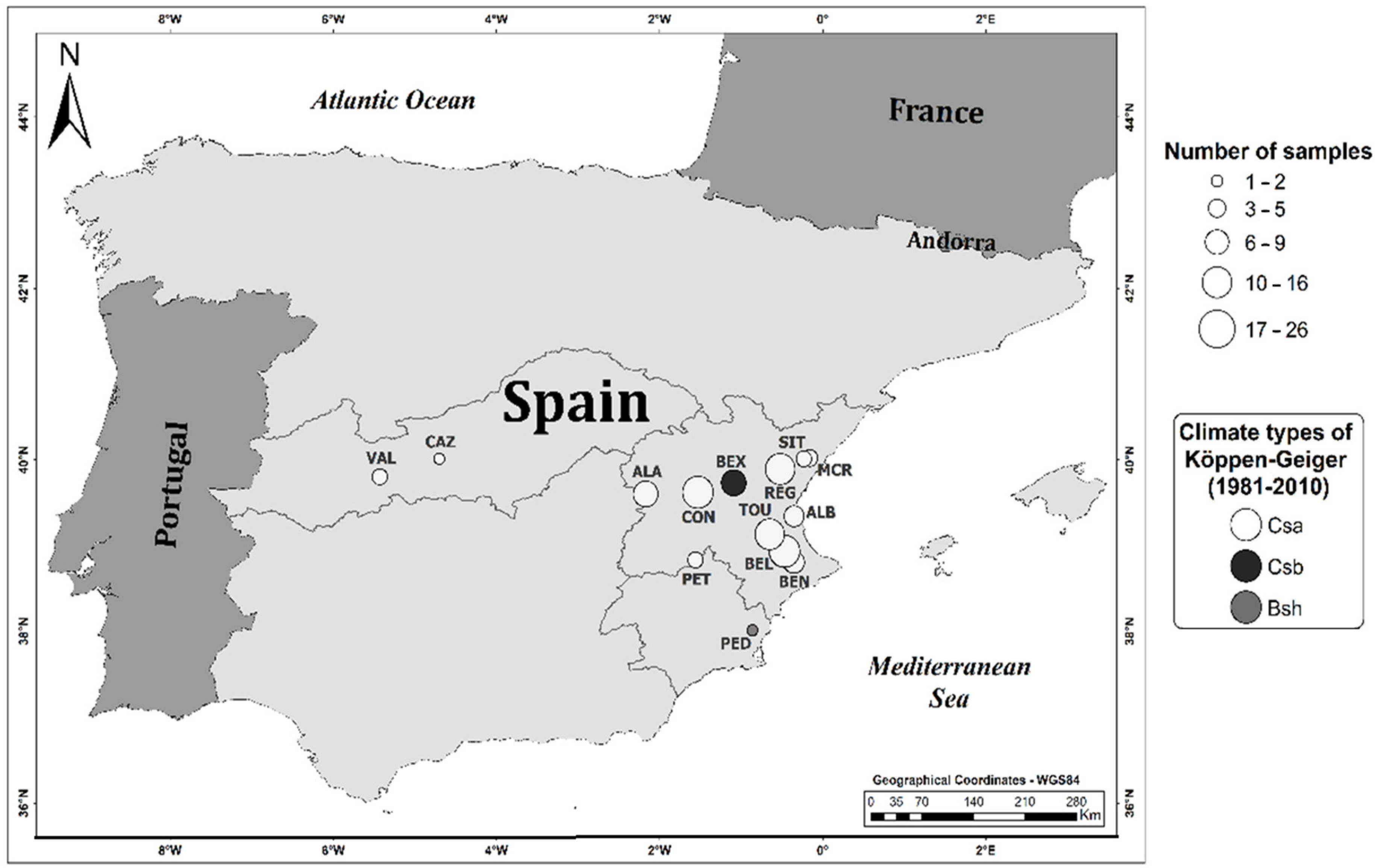
Merging the databases of two recent projects has provided us with a large amount of data to carry out the validation of Rrs and water quality algorithms. The database covers a wide gradient of limnological variables but is always within the wide range used to develop the algorithms. It is a database representative of the variability of the climatic and limnological conditions of the Mediterranean Basin, with a greater representation of semi-arid environments.

Regarding cross-correlations between the variables, similar to the data used to develop the water quality algorithms by in situ spectrometry, the OACs mainly affecting water transparency are TSS and phytoplankton pigments and as a consequence, have greater influence on the spectra of the studied water bodies, while CDOM has less influence on water transparency and the spectral features of the dataset. This higher or lower influence on the water spectrum facilitates or hinders its determination through remote sensing.

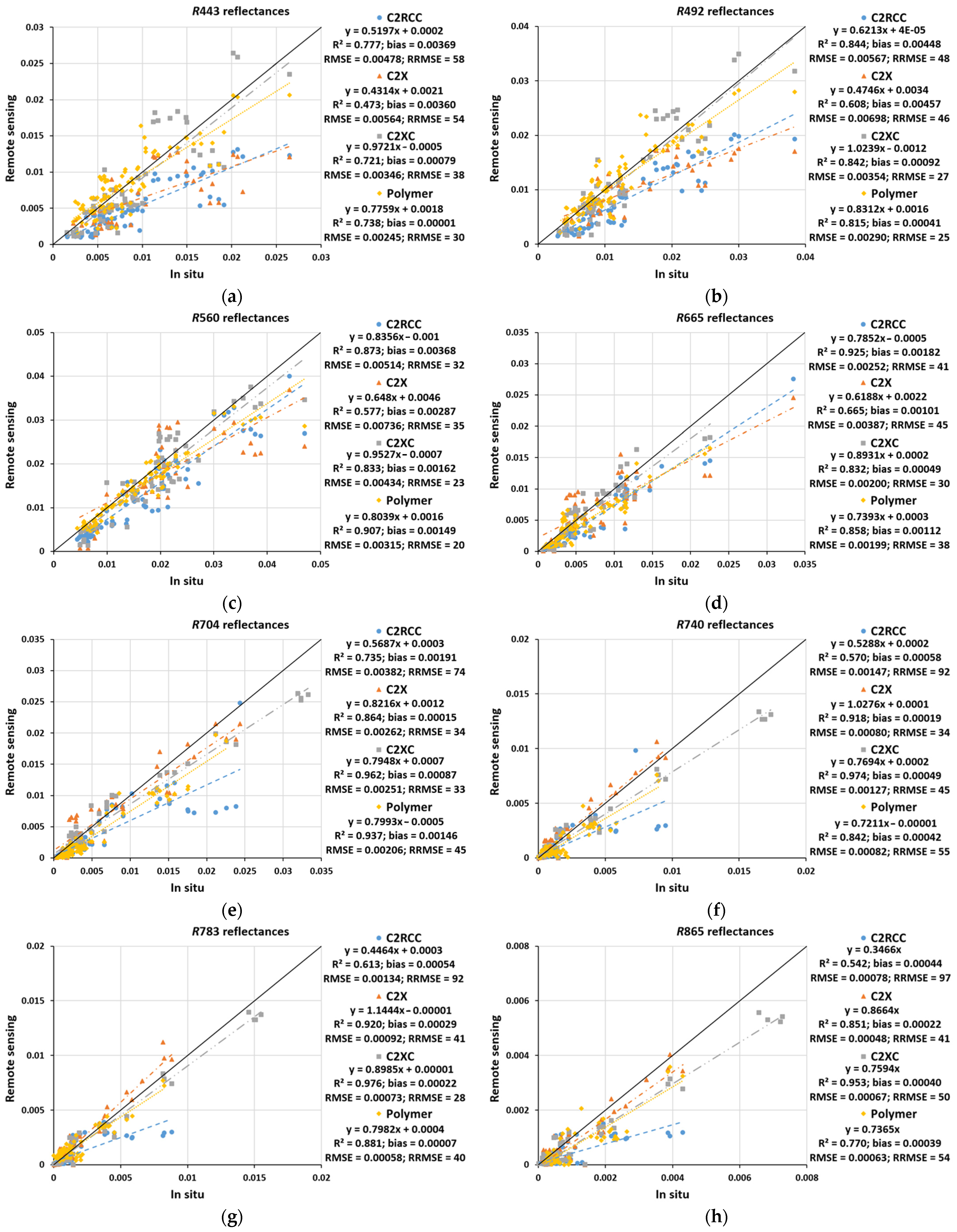
Rrs validation has been performed for four types of ACs, three of them, the C2-Nets based on NN, and Polymer, a physical model based on a spectral optimization method. The C2-Nets use the top-of-atmosphere full spectrum as the input, while Polymer recovers the radiation scattered and absorbed by water from the measured signal by satellite sensors from the blue to the near-infrared spectral range.

Considering the ACs models characteristics tested with our data and the validation results, with the Polymer program, we obtain the best validation results for the visible region, precisely the spectrum part used to apply the spectral matching method, and the worst in the NIR according to Pereira-Sandoval et al. [12], Warren et al. [20], and Caballero et al. [33].

Regarding the C2-Nets, using the top-of-atmosphere full spectrum as the input, except for C2RCC, both C2X and C2XC obtain better validation results than Polymer in the Red-edge and NIR bands. C2-Nets differences are consistent in the used trained ranges of IOPs. With our data, the C2-Net, C2XC-using intermediate IOPs ranges achieve the best validation results for all bands, except for R740 and R865, whose best results are obtained with C2X. C2X improves its results for longer wavelength bands because its trained ranges of scattering coefficients of typical sediments and white particles (calcareous sediments) include extreme cases, better reproducing the increased scattering in the NIR and demonstrating their best results for turbid waters, agreeing with Pereira-Sandoval et al. [12], Pahlevan et al. [34], and Tavares et al. [35].

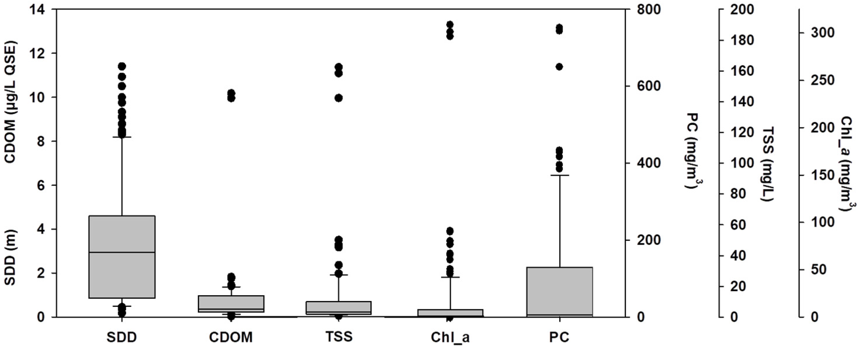
Another important aspect to take into account is the restrictiveness of the respective quality flags. According to this criterion, the Polymer program has obtained the highest number of match-ups with respect to the other ACs, according to Steinmetz et al. [17], Caballero et al. [33], Warren et al. [20], Pereira-Sandoval et al. [12], and Bui et al. [21]. Regarding C2-Nets, applying quality flags and match-up exercises, fewer data were removed with C2RCC because it is trained for a lower IOPs range and coastal waters, and as can be seen in Figure 2, most of the samples have low concentrations of IOPs. However, its validation results were the worst for all bands except for R560 and R665, for which C2X had the worst results. Meanwhile, the most restrictive AC, and therefore the one with fewer data for the validation process, was C2X because it is trained for a high IOPs range, and our dataset has few samples with high IOPs concentrations. Therefore, for our dataset, the reduced number of valid match-ups and lower consistency in the accuracy along the spectrum observed with this processor made it the most uncertain C2-Net, agreeing with Soriano-González et al. [32]. These results indicate that the C2-Nets development is improving and adapting their training range for inland waters, although the sun glint handicap has not yet been solved.

The results illustrate well that the ACs developed from NN are more limited to the water conditions of their training database. Polymer may also have limitations due to its internal marine model, depending on chlorophyll and sediments, although its present high performance shows suitability for our water types. The inconvenience with Polymer is the difficulty to process images for a non-professional user since it is not a program with a user-friendly interface.

Regarding the water quality algorithms validation, the best results were obtained with the ACs with the best Rrs validation results, C2XC and Polymer. The best-validated algorithm for SDD estimation uses the Blue/Green ratio (R492/R560) applied to Polymer Rrs. It is the algorithm with the shortest wavelength bands of all tested algorithms, and therefore the bands with the fewest errors in the validation of the Rrs. The Blue/Green ratio was the second-best result in the previous study, with results very similar to ours, with an R² of 0.65, an RMSE of 1.21 m, an RRMSE of 51%, and a bias of 0.47 m, which were obtained for a 0.14–9.55 m range. In our validation results, the RMSE is slightly higher (1.59 m), although the RRMSE is lower (47%) for the same range of data. The results also agree with the RMSE of 1.4 m obtained with 82 samples in the study carried out by Delegido et al. [36], using the same AC and relation bands. The good results also obtained with C2XC (Table A2) indicate that the algorithm obtained from 266 in situ reflectances is applicable and reliable for ACs that achieve an accurate estimate of water-leaving radiance.

The best-validated algorithm for CDOM estimation, based on the Red-edge1/Blue ratio (R704/R492) and applied to C2XC Rrs, was the algorithm with the biggest errors in the previous study. However, the validation results were very similar among the different algorithms on the previous study, obtaining for R704/R492 ratio an R² of 0.5, an RMSE of 1.03 µg/L QSE, an RRMSE of 56% and a bias of 0.26 µg/L QSE, for a data range between 0.3 and 5.3 µg/L QSE. The values improved in our validation for R² (0.8) and RMSE (0.42 µg/L QSE), while the bias (0.32 µg/L QSE) is similar and the RRMSE (87%) is much higher because the range of data is much lower, 0.03–1.75 µg/L QSE. These results are in agreeance with bands relations obtained in the study carried out by Ruescas et al. [37], from simulated water-leaving radiance by Hydrolight and with the potential correlation between the Rrs and CDOM values obtained in Kutser et al. [38], Kutser [39], Slonecker et al. [40], and Chen et al. [41]. The bad results in contrast to the other variables could be due to the lesser influence of CDOM on the transparency for our database and consequently in the reflectance spectrum. Nevertheless, although the RMSE seems low, the algorithm should be tested with a larger CDOM range.

For TSS, in situ reflectance algorithms for two data ranges were validated, below and above 20 mg/L, and in both groups, the best algorithm was obtained using the R704 band and Polymer Rrs. Both algorithms are obtained with a lineal calibration correlation, but the slopes and offsets are very different. Of all the bands used in the tested algorithms, R704 is not simply the band with lowest errors in the validation of the Rrs but it is the band with better results in the previous study. The best validation results for values below 20 mg/L in the Previous Study were also with R704 band, with an R² of 0.85, an RMSE of 1.79 mg/L, an RRMSE of 43%, and a bias of 0.39 mg/L, very similar values to those obtained in this work, where all the validation results enhance except bias (0.74 mg/L). On the other hand, for values above 20 mg/L, with only five data points available for validation in the previous study, the R704 band did not reach the best results. With these five data points, only an R² of 0.02, an RMSE of 85.97 mg/L, an RMSE of 190%, and a bias of 20.82 mg/L were obtained. The results greatly improved in this work, using 13 data points in the validation process. The results are in agreeance with Soomets el al.’s [42] study, using TOA, C2RCC, and C2X ACs according the optical water type.

The other variable with two algorithms was Chl_a, but this time, the algorithms were not coincidental for concentrations above and below 5 mg/m³. The threshold value was 5 mg/m³ because waters with high Chl_a (above 3–5 mg/m³ [43]) produce discernible spectral features in the red and NIR regions of the reflectance spectrum [44]. The best algorithm for values below 5 mg/m³ was the same as that obtained in the previous study, the log₁₀ of the ratio between the band with a maximum value among the R443 and R492 bands as the numerator and R560 as the denominator using C2XC Rrs, the bands with the fewest errors in the validation of the Rrs. The validation results in the previous study were an R² of 0.55, an RMSE of 0.94 mg/m³, an RRMSE of 43%, and a bias of 0.09 mg/L, similar values to that obtained in this work, where the validation results enhance the RMSE of 0.93 mg/m³ and the bias of 0.01 mg/m³. The second-best result was obtained with Polymer Rrs, with the AC having the better validation results for the used bands, obtaining an RMSE of 1.04 mg/m³, only 0.1 mg/m³ higher than the previous study validation results but with a very high RRMSE of 64%. The RRMSE is higher as the number of data below 2 mg/m³ increases, with 72% of the data points in the Polymer validation in front of the 66% in the C2XC validation and the 56% in the previous study. These results are in agreement with the study carried out by Pereira-Sandoval et al. [12], obtaining an absolute error of 0.89 mg/m³. The results corroborate the applicability of the algorithm developed by O’Reilly and Werdell [5] for hyperspectral sensors using in situ radiometry in multispectral sensors using atmospherically corrected MSI Rrs.

The best algorithm for values above 5 mg/m³ was the Green/Red ratio (R560/R665) applied to Polymer Rrs, although in the previous study, the validation results of this algorithm using in situ Rrs were bad, with an R² of 0, an RMSE of 144 mg/m³, an RRMSE of 156%, and a bias of 43 mg/m³. However, the algorithm generated with 144 data points in the previous study applied to the 42 data used in the Polymer validation provided the best validation results, an R² of 0.9, an RMSE of 28.1 mg/m³, an RRMSE of 50%, and a bias of 1.35 mg/m³. This result may be due to two factors, (1) the data range and (2) the used bands. Regarding data range, only 4 of the 42 data used were higher than 100 mg/m³, and in the previous study, the RMSE for the R560/R665 ratio would be 34.72 mg/m³ using only values lower than 100 mg/m³. Regarding the used bands, the R560/R665 ratio was the one that used the shortest wavelength bands of all the tested algorithms using concentrations higher than 5 mg/m³, the wavelengths for which Polymer gives the best results in the validation of the Rrs. The band relation corresponds to the ratio between reflectances at the minimum absorption at the green region between 550 and 555 nm, to reflectances at the second peak absorption at the red region between 670 and 675 nm, used by Ha et al. [45] in S2-MSI images using the empirical line method as an AC and obtaining a standard error of 0.14 mg/m³ for a data range of 1.58–6.00 mg/m³. The same equation was used by Pereira et al. [46], obtaining an RMSE of 21.9 for a larger data range of 4.14–76.44 mg/m³, increasing the RMSE with the data range. It is noted that for C2X and C2XC, using only 13 and 17 data, respectively, the best algorithm obtained was the three-band model of Dall’Olmo et al. [47], using the R740, R704, and R665 bands, for which C2X and C2XC were the ACs with the best validation results. A three-band model obtained the fourth best validation result in the previous study, with an R² of 0.85, an RMSE of 41.8 mg/m³, an RRMSE of 52%, and a bias of 4.77 mg/m³, while for the C2XC Rrs validation results, the R² was 0.9, the RSME was 50.6 mg/m³, the RRMSE was 57%, and the bias was 3.22 mg/m³. This RMSE is similar to that obtained by Cairo et al. [48] of 56.9 mg/m³ in his study using the three-band model, the 6S (Second Simulation of the Satellite Signal in the Solar Spectrum) model for AC, and a Chl_a data range until 600 mg/m³, and an RMSE slightly higher than that obtained by Ogashawara et al. [49] of 33.5 mg/m³ for a data range between 2.3 and 306 mg/m³. It may be that an improved recovery of the Red-edge bands with Polymer will make the three-band model the best Chl_a retrieval algorithm.

The best-validated algorithm for PC estimation was based on the Red-edge1/Red ratio (R704/R665) and applied to C2XC Rrs. The Red-edge1/Red ratio was the algorithm with the shortest wavelength bands of all tested algorithms, and therefore the bands with the fewest errors in the validation of the Rrs, and it was also the best result in the previous study. The validation results in the previous study were an R² of 0.8, an RMSE of 43.7 mg/m³, an RRMSE of 55%, and a bias of 14.64 mg/m³ for a data range between 0.7 and 1040 mg/m³. The results improved in this work with an R² of de 0.9, an RMSE of 38.9 mg/m³, an RRMSE of 39%, and a bias of 5.45 mg/m³ for a data range between 0 and 751.1 mg/m³. This demonstrates the band ratio applicability in S2-MSI images, which is a band ratio used in the previous study and in the drone and aircraft studies of Kwon et al. [50] and Beck et al. [51]. The calculated RMSE is similar to the standard error of 45.5 mg/m³ obtained by Simis et al. [2] for a PC higher than 50 mg/m³, using samples from the same climatic region.

The application of water quality algorithms developed from in situ reflectances, using reflectances obtained after an AC process, may lead to different errors than those calculated in the development of the algorithms. Algorithms with the shortest wavelength bands had better results if their validation results in the previous study were not very high. Only three algorithms were coincident and showed similar error statistics. However, the results demonstrate the applicability of the algorithms developed from in situ reflectances to satellite S2-MSI imagery after the correction of atmospheric and sun specular effects, a step that was missing in other works.

Indeed, there is always some difficulty to obtain general algorithms to cover a wide range of data. One solution to obtain a good retrieval algorithm for each different bio-optical variable is to obtain specific algorithms for each different water type according to a pre-established classification based on their optical spectrum (optical water types), as it has been performed in several studies (e.g., Moore et al. [52]; Neil et al. [53]; Uudeberg et al. [19]; Soomets et al. [42]). If the same problem exists for AC, the results would probably be more accurate if the optical water type differentiation was defined before applying the AC.

5. Conclusions

Regarding the Rrs validation, the results have shown that the best ACs tested in this work were C2XC and Polymer. The Polymer program estimated most accurately the water-leaving radiance of the visible region, while C2XC estimated more accurately the Red-edge region and C2X NIR band. However, on the one hand, it should be noted that C2XC and C2X remove more data, and on the other hand, they are easier to use than the Polymer program for non-professional users due to their integration in the SNAP program.

Despite the difficulties to obtain the same algorithms as in the previous study after validation with estimated Rrs, the results were coincident for three algorithms: TSS below 20 mg/L, Chl_a below 5 mg/m³, and PC. Even the validation results for the PC and TSS below 20 mg/L improved. With regard to the bands used, the best validation results for SDD and PC were found using the Rrs of the ACs that obtained the best validation results for the bands used by the specific algorithm.

The best results after the algorithm validation were obtained using the Rrs of the Polymer and C2XC; the ACs with the best validation results correlate to the in situ and remote sensing reflectance data for each band.

From the results obtained, the best water quality algorithm and the most adequate AC can be chosen to carry out the spatial and temporal monitoring of a water body, either for its management or for the performance of applied remote sensing studies using S2-MSI imagery.

References

1. Navalgund, R.R.; Jayaraman, V.; Roy, P.S. Remote sensing applications: An overview. Curr. Sci. 2007, 93, 1747–1766. [Google Scholar]
2. Simis, S.G.; Ruiz-Verdú, A.; Domínguez-Gómez, J.A.; Peña-Martinez, R.; Peters, S.W.; Gons, H.J. Influence of phytoplankton pigment composition on remote sensing of cyanobacterial biomass. Remote Sens. Environ. 2007, 106, 414–427. [Google Scholar] [CrossRef]
3. Brezonik, P.L.; Olmanson, L.G.; Finlay, J.C.; Bauer, M.E. Factors affecting the measurement of CDOM by remote sensing of optically complex inland waters. Remote Sens. Environ. 2015, 157, 199–215. [Google Scholar] [CrossRef]
4. Lins, R.C.; Martinez, J.M.; Motta Marques, D.D.; Cirilo, J.A.; Fragoso, C.R. Assessment of chlorophyll-a remote sensing algorithms in a productive tropical estuarine-lagoon system. Remote Sens. 2017, 9, 516. [Google Scholar] [CrossRef]
5. O’Reilly, J.E.; Werdell, P.J. Chlorophyll algorithms for ocean color sensors-OC4, OC5 & OC6. Remote Sens. Environ. 2019, 229, 32–47. [Google Scholar] [PubMed]
6. Sòria-Perpinyà, X.; Vicente, E.; Urrego, P.; Pereira-Sandoval, M.; Tenjo, C.; Ruíz-Verdú, A.; Delegido, J.; Soria, J.M.; Peña, R.; Moreno, J. Validation of water quality monitoring algorithms for sentinel-2 and sentinel-3 in Mediterranean inland waters with in situ reflectance data. Water 2021, 13, 686. [Google Scholar] [CrossRef]
7. Gordon, H.R. Calibration requirements and methodology for remote sensors viewing the ocean in the visible. Remote Sens. Environ. 1987, 22, 103–126. [Google Scholar] [CrossRef]
8. Wang, M. Atmospheric correction for remotely-sensed ocean-colour products. In Reports and Monographs of the International Ocean-Colour Coordinating Group (IOCCG); International Ocean Colour Coordinating Group (IOCCG): Dartmouth, NS, Canada, 2010. [Google Scholar]
9. Gordon, H.R.; Wang, M. Retrieval of water-leaving radiance and aerosol optical thickness over the oceans with SeaWiFS: A preliminary algorithm. Appl. Opt. 1994, 33, 443–452. [Google Scholar] [CrossRef]
10. Martins, V.S.; Barbosa, C.C.F.; de Carvalho, L.A.S.; Jorge, D.S.F.; Lobo, F.D.L.; Novo, E.M.L.D.M. Assessment of atmospheric correctionmethods for Sentinel-2MSI images applied to Amazon floodplain lakes. Remote Sens. 2017, 9, 322. [Google Scholar] [CrossRef]
11. Pereira-Sandoval, M.; Urrego, P.; Ruiz-Verdú, A.; Tenjo, C.; Delegido, J.; Soria-Perpinyà, X.; Vicente, E.; Soria, J.; Moreno, J. Calibration and validation of algorithms for the estimation of chlorophyll-a concentration and Secchi depth in inland waters with Sentinel-2. Limnetica 2019, 38, 471–487. [Google Scholar] [CrossRef]
12. Qian, S.E. Hyperspectral Satellites and System Design, 1st ed.; CRC Press: Boca Raton, FL, USA, 2020; p. 626. [Google Scholar]
13. Wang, M. Atmospheric correction of Ocean Color RS observations. In Proceedings of the IOCCG Summer Lecture Series, Villefranche-sur-Mer, France, 21 July–2 August 2014; pp. 1–58. [Google Scholar]
14. Soria, X.; Delegido, J.; Urrego, P.; Pereira-Sandoval, M.; Vicente, E.; Ruiz-Verdú, A.; Soria, J.M.; Peña, R.; Tenjo, C.; Moreno, J. Validación de algoritmos para la estimación de la clorofila-a con Sentinel-2 en la Albufera de València. In Proceedings of the XVII Congreso de la Asociación Española de Teledetección, Murcia, Spain, 3–7 October 2017; pp. 289–292. [Google Scholar]
15. Doerffer, R.; Schiller, H. The MERIS Case 2 water algorithm. Int. J. Remote Sens. 2007, 28, 517–535. [Google Scholar] [CrossRef]
16. Steinmetz, F.; Ramon, D. Sentinel-2 MSI and Sentinel-3 OLCI consistent ocean colour products using POLYMER. In Proceedings of the Remote Sensing of the Open and Coastal Ocean and Inland Waters, Honolulu, HI, USA, 24–25 September 2018; Volume 10778, p. 107780E. [Google Scholar]
17. Steinmetz, F.; Deschamps, P.-Y.; Ramon, D. Atmospheric correction in presence of sun glint: Application to MERIS. Opt. Express 2011, 19, 9783–9800. [Google Scholar] [CrossRef] [PubMed]
18. Ansper, A.; Alikas, K. Retrieval of chlorophyll a from Sentinel-2 MSI data for the European Union water framework directive reporting purposes. Remote Sens. 2019, 11, 64. [Google Scholar] [CrossRef]
19. Uudeberg, K.; Ansko, I.; Põru, G.; Ansper, A.; Reinart, A. Using optical water types to monitor changes in optically complex inland and coastal waters. Remote Sens. 2019, 11, 2297. [Google Scholar] [CrossRef]
20. Warren, M.A.; Simis, S.G.; Martinez-Vicente, V.; Poser, K.; Bresciani, M.; Alikas, K.; Spyrakos, E.; Giardino, C.; Ansper, A. Assessment of atmospheric correction algorithms for the Sentinel-2A MultiSpectral Imager over coastal and inland waters. Remote Sens. Environ. 2019, 225, 267–289. [Google Scholar] [CrossRef]
21. Bui, Q.T.; Jamet, C.; Vantrepotte, V.; Mériaux, X.; Cauvin, A.; Mograne, M.A. Evaluation of sentinel-2/MSI atmospheric correction algorithms over two contrasted French coastal waters. Remote Sens. 2022, 14, 1099. [Google Scholar] [CrossRef]
22. Vicente, E.; Hoyos, C.; Sánchez, P.; Cambra, J. Metodología para el Establecimiento el Estado Ecológico según la Directiva Marco del Agua. Protocolos de Muestreo y Análisis para Fitoplancton [Methodology for Establishing the Ecological Status according to the Water Framework Directive. Sampling Protocols and Analysis for Phytoplankton]; Confederación Hidrográfica del Ebro, Ministerio de Medio Ambiente: Zaragoza, Spain, 2005. [Google Scholar]
23. Mobley, C.D. Estimation of the remote-sensing reflectance from above-surface measurements. Appl. Opt. 1999, 38, 7442–7455. [Google Scholar] [CrossRef]
24. European Space Agency. Sentinel-2 Spectral Response Functions (S2-SRF) v3.0. Available online: https://earth.esa.int/web/sentinel/user-guides/sentinel-2-msi/document-library/-/asset_publisher/Wk0TKajiISaR/content/sentinel-2a-spectralresponses (accessed on 16 April 2020).
25. Shoaf, W.T.; Lium, B.W. Improved extraction of chlorophyll a and b from algae using dimethyl sulphoxide. Limnol. Oceanogr. 1976, 21, 926–928. [Google Scholar] [CrossRef]
26. Jeffrey, S.T.; Humphrey, G.F. New spectrophotometric equations for determining chlorophylls a, b, c1 and c2 in higher plants, algae and natural phytoplankton. Biochem. Physiol. Pflanz. 1975, 167, 191–194. [Google Scholar] [CrossRef]
27. Korshin, G.V.; Li, C.W.; Benjamin, M.M. Monitoring the properties of natural organic matter through UV spectroscopy: A consistent theory. Water Res. 1997, 31, 1787–1795. [Google Scholar] [CrossRef]
28. ESA. Sentinel-2: ESA’s Optical High-Resolution Mission for GMES Operational Services; Fletcher, K., Ed.; ESA Communications: Noordwijk, The Netherlands, 2012. [Google Scholar]
29. Pan, Y.; Bélanger, S.; Huot, Y. Evaluation of atmospheric correction algorithms over lakes for high-resolution multispectral imagery: Implications of adjacency effect. Remote Sens. 2022, 14, 2979. [Google Scholar] [CrossRef]
30. Brockmann, C.; Doerffer, R.; Peters, M.; Stelzer, K.; Embacher, S.; Ruescas, A. Evolution of the C2RCC neural network for Sentinel 2 and 3 for the retrieval of ocean colour products in normal and extreme optically complex waters. In Proceedings of the Living Planet Symposium 2016, Prague, Czech Republic, 9–13 May 2016. [Google Scholar]
31. C2X-Complex. ESA Step Forum. Available online: https://forum.step.esa.int/t/c2x-complex/29392 (accessed on 27 September 2021).
32. Soriano-González, J.; Urrego, E.P.; Sòria-Perpinyà, X.; Angelats, E.; Alcaraz, C.; Delegido, J.; Ruíz-Verdú, A.; Tenjo, C.; Vicente, E.; Moreno, J. Towards the combination of C2RCC processors for improving water quality retrieval in inland and coastal areas. Remote Sens. 2022, 14, 1124. [Google Scholar] [CrossRef]
33. Caballero, I.; Steinmetz, F.; Navarro, G. Evaluation of the first year of operational Sentinel-2A data for retrieval of suspended solids in medium-to high-turbidity waters. Remote Sens. 2018, 10, 982. [Google Scholar] [CrossRef]
34. Pahlevan, N.; Mangin, A.; Balasubramanian, S.V.; Smith, B.; Alikas, K.; Arai, K.; Barbosa, C.; Bélanger, S.; Binding, C.; Bresciani, M.; et al. ACIX-Aqua: A global assessment of atmospheric correction methods for Landsat-8 and Sentinel-2 over lakes, rivers, and coastal waters. Remote Sens. Environ. 2021, 258, 112366. [Google Scholar] [CrossRef]
35. Tavares, M.H.; Lins, R.C.; Harmel, T.; Fragoso, C.R.; Martínez, J.M.; Motta-Marques, D. Atmospheric and sunglint correction for retrieving chlorophyll-a in a productive tropical estuarine-lagoon system using Sentinel-2 MSI imagery. ISPRS J. Photogramm. Remote Sens. 2021, 174, 215–236. [Google Scholar] [CrossRef]
36. Delegido, J.; Urrego, P.; Vicente, E.; Sòria-Perpinyà, X.; Soria, J.M.; Pereira-Sandoval, M.; Ruiz-Verdú, A.; Peña, R.; Moreno, J. Turbidez y profundidad de disco de Secchi con Sentinel-2 en embalses con diferente estado trófico en la Comunidad Valenciana. Rev. Teledetec. 2019, 54, 15–24. [Google Scholar] [CrossRef]
37. Ruescas, A.B.; Hieronymi, M.; Mateo-Garcia, G.; Koponen, S.; Kallio, K.; Camps-Valls, G. Machine learning regression approaches for colored dissolved organic matter (CDOM) retrieval with S2–MSI and S3–OLCI simulated data. Remote Sens. 2018, 10, 786. [Google Scholar] [CrossRef]
38. Kutser, T.; Pierson, D.C.; Kallio, K.Y.; Reinart, A.; Sobek, S. Mapping lake CDOM by satellite remote sensing. Remote Sens. Environ. 2005, 94, 535–540. [Google Scholar] [CrossRef]
39. Kutser, T. The possibility of using the Landsat image archive for monitoring long time trends in coloured dissolved organic matter concentration in lake waters. Remote Sens. Environ. 2012, 123, 334–338. [Google Scholar] [CrossRef]
40. Slonecker, E.T.; Jones, D.K.; Pellerin, B.A. The new Landsat 8 potential for remote sensing of colored dissolved organic matter (CDOM). Mar. Pollut. Bull. 2016, 107, 518–527. [Google Scholar] [CrossRef]
41. Chen, J.; Zhu, W.; Pang, S.; Cheng, Q. Applicability evaluation of Landsat-8 for estimating low concentration colored dissolved organic matter in inland water. Geocarto Int. 2022, 37, 1–15. [Google Scholar] [CrossRef]
42. Soomets, T.; Uudeberg, K.; Jakovels, D.; Brauns, A.; Zagars, M.; Kutser, T. Validation and comparison of water quality products in baltic lakes using Sentinel-2 MSI and Sentinel-3 OLCI data. Sensors 2020, 20, 742. [Google Scholar] [CrossRef] [PubMed]
43. Gitelson, A.; Dall’Olmo, G.; Moses, W.; Rundquist, D.; Barrow, T.; Fisher, T.; Gurlin, D.; Holz, J. A simple semi-analytical model for remote estimation of chlorophyll-a in turbid waters: Validation. Remote Sens. Environ. 2008, 112, 3582–3593. [Google Scholar] [CrossRef]
44. Moses, W.J.; Saprygin, V.; Gerasyuk, V.; Povazhnyy, V.; Berdnikov, S.; Gitelson, A.A. OLCI-based NIR-red models for estimating chlorophyll-a concentration in productive coastal waters—A preliminary evaluation. Environ. Res. Commun. 2019, 1, 011002. [Google Scholar] [CrossRef]
45. Ha, N.T.T.; Thao, N.T.P.; Koike, K.; Nhuan, M.T. Selecting the best band ratio to estimate chlorophyll-a concentration in a tropical freshwater lake using sentinel 2A images from a case study of Lake Ba Be (Northern Vietnam). ISPRS Int. J. Geo-Inf. 2017, 6, 290. [Google Scholar] [CrossRef]
46. Pereira, A.R.A.; Lopes, J.B.; Espindola, G.M.D.; Silva, C.E.D. Retrieval and mapping of chlorophyll-a concentration from Sentinel-2 images in an urban river in the semiarid region of Brazil. Rev. Ambient. Água 2020, 15. [Google Scholar] [CrossRef]
47. Dall’Olmo, G.; Gitelson, A.; Rundquist, D. Towards a unified approach for remote estimation of chlorophyll-a in both terrestrial vegetation and turbid productive waters. Geophys. Res. Lett. 2003, 30, 1938. [Google Scholar] [CrossRef]
48. Cairo, C.; Barbosa, C.; Lobo, F.; Novo, E.; Carlos, F.; Maciel, D.; Flores Júnior, R.; Silva, E.; Curtarelli, V. Hybrid chlorophyll-a algorithm for assessing trophic states of a tropical Brazilian reservoir based on MSI/Sentinel-2 data. Remote Sens. 2020, 12, 40. [Google Scholar] [CrossRef]
49. Ogashawara, I.; Kiel, C.; Jechow, A.; Kohnert, K.; Ruhtz, T.; Grossart, H.P.; Hölker, F.; Nejstgaard, J.C.; Berger, S.A.; Wollrab, S. The use of Sentinel-2 for chlorophyll-a spatial dynamics assessment: A comparative study on different lakes in northern Germany. Remote Sens. 2021, 13, 1542. [Google Scholar] [CrossRef]
50. Kwon, Y.S.; Pyo, J.; Kwon, Y.H.; Duan, H.; Cho, K.H.; Park, Y. Drone-based hyperspectral remote sensing of cyanobacteria using vertical cumulative pigment concentration in a deep reservoir. Remote Sens. Environ. 2020, 236, 111517. [Google Scholar] [CrossRef]
51. Beck, R.; Xu, M.; Zhan, S.; Liu, H.; Johansen, R.A.; Tong, S.; Yang, B.; Shu, S.; Wu, Q.; Wang, S.; et al. Comparison of satellite reflectance algorithms for estimating phycocyanin values and cyanobacterial total biovolume in a temperate reservoir using coincident hyperspectral aircraft imagery and dense coincident surface observations. Remote Sens. 2017, 9, 538. [Google Scholar] [CrossRef] [Green Version]
52. Moore, T.S.; Dowell, M.D.; Bradt, S.; Verdu, A.R. An optical water type framework for selecting and blending retrievals from bio-optical algorithms in lakes and coastal waters. Remote Sens. Environ. 2014, 143, 97–111. [Google Scholar] [CrossRef] [PubMed]
53. Neil, C.; Spyrakos, E.; Hunter, P.D.; Tyler, A.N. A global approach for chlorophyll-a retrieval across optically complex inland waters based on optical water types. Remote Sens. Environ. 2019, 229, 159–178. [Google Scholar] [CrossRef]
Figure 1. Location of sampled lakes and reservoirs. Symbol size reflects the number of samples collected at each site, and grayscale reflects the climate type.
Remotesensing 14 04794 g001
Figure 2. Boxplot of the values range for the water quality parameters. The box bounds the interquartile range (IQR; 25–75 percentile), the horizontal line inside the box indicates the median, and the whiskers (error bars) indicate the 90th above and 10th below percentiles. Dots indicate the outliers.
Remotesensing 14 04794 g002
Figure 3. Linear correlations between the in situ and remote sensing reflectance data for the different S2-MSI bands and respective validation statistics results, using 81 samples for C2RCC, 41 for C2X, 55 for C2XC, and 92 for Polymer. RMSE and bias in sr−1 and RRMSE in %.
Remotesensing 14 04794 g003