1. Introduction
The radar micro-Doppler (m-D) effect describes the frequency shift phenomenon induced by targets or components of targets undergoing micro-motion dynamics [
1]. For a target with multiple scattering centers, the individual micro-motion of the scattering centers is different. The radar echo contains several m-D components [
2]. By separating m-D components or estimating the m-D from the radar echo, Doppler features corresponding to the specific target parts can be extracted, and target fine status analysis can therefore be achieved [
3]. It is noted that the m-D signal is typically a multicomponent non-stationary signal, and the m-Ds of the target’s scattering centers are identical to the signal’s instantaneous frequencies (IFs) when the target’s motion only contains micro-motion, which is the major studied scenario in existing research.
Numerous m-D signal estimation methods were proposed, which can be divided into signal-based and image-based methods. The signal-based methods decompose the radar echo into a set of statistically uncorrelated or independent components [
4] by using techniques such as Empirical Mode Decomposition [
5], Variational Mode Decomposition [
6], Singular Value Decomposition [
7] and Independent Component Analysis [
8]. After obtaining the individual components, their IFs can be estimated. However, most signal-based methods assume that the signal components comply with certain separation conditions.
The image-based methods are based on time–frequency representation (TFR). As TFR can characterize the echo signal in time and frequency dimensions, it is widely used for m-D feature extraction. The m-D signal presents multiple continuous ridges in the TFR. Thus, the m-D can be estimated by applying curve detection methods. Hough transform (HT) [
9] and inverse radon transform (IRT) [
10] extract m-D components by carrying out a peak selecting procedure in transform space. These two methods work well in extracting cross components even if strong noise exists, but the m-D model needs to be preset, which has limitations in real-world scenarios, where the m-D model is unknown as a prior or if there is a derivation between the real m-D and its model. The Viterbi algorithm (VA) and its improved version [
11] perform m-D component extraction by detecting curves on the TFR by setting the path connection penalty function. However, VA-based methods are computationally expensive. Ridge detection and tracking methods are computationally efficient alternatives to the VA. The ridge path regrouping algorithm (RPRG) detects and regroups components based on the slope of IF at the intersection region [
12], but it is sensitive to noise. The adaptive directional time–frequency distribution-based ridge tracking (ADTFD-RT) method estimates the IF of components along the direction of the principal axis of ridges [
13], yet the improved performance is achieved at the expense of additional calculation costs.
Higher-dimensional signal characterization is a new way to achieve signal extraction. It is possible to separate signals that overlap in the time–frequency plane in high-dimensional feature space [
14,
15]. The frequency-chirprate reassignment method (FCRM) makes the crossing components appear separated in the time–frequency-chirprate domain [
14], but its accuracy is easily influenced by the scaling factor. A more robust three-dimensional extracting transform (TET) based on chirplet transform is proposed to obtain perfect IF estimation[
15]. However, the 3D representation requires a tremendous amount of computation.
Although the above methods perform well in certain conditions, they are mainly confronted with three challenges: (1) The overlapping m-D components are difficult to extract; (2) The used model based on a prior cannot adapt to various m-D components such as non-sinusoidal and irregular forms. (3) Performance is degraded for scenarios where there exists strong noise.
The booming of deep learning technology advances the performance of radar target detection [
16], recognition [
17] and imaging [
18] in real applications. However, it is rare in radar signal separation and extraction. Semantic line detection is a time-honored problem in computer vision, which aims to find meaningful lines with strong shapes with prior knowledge but weak apparent coherence [
19]. It was widely used in computer vision tasks such as lane detection [
20] and image aesthetics [
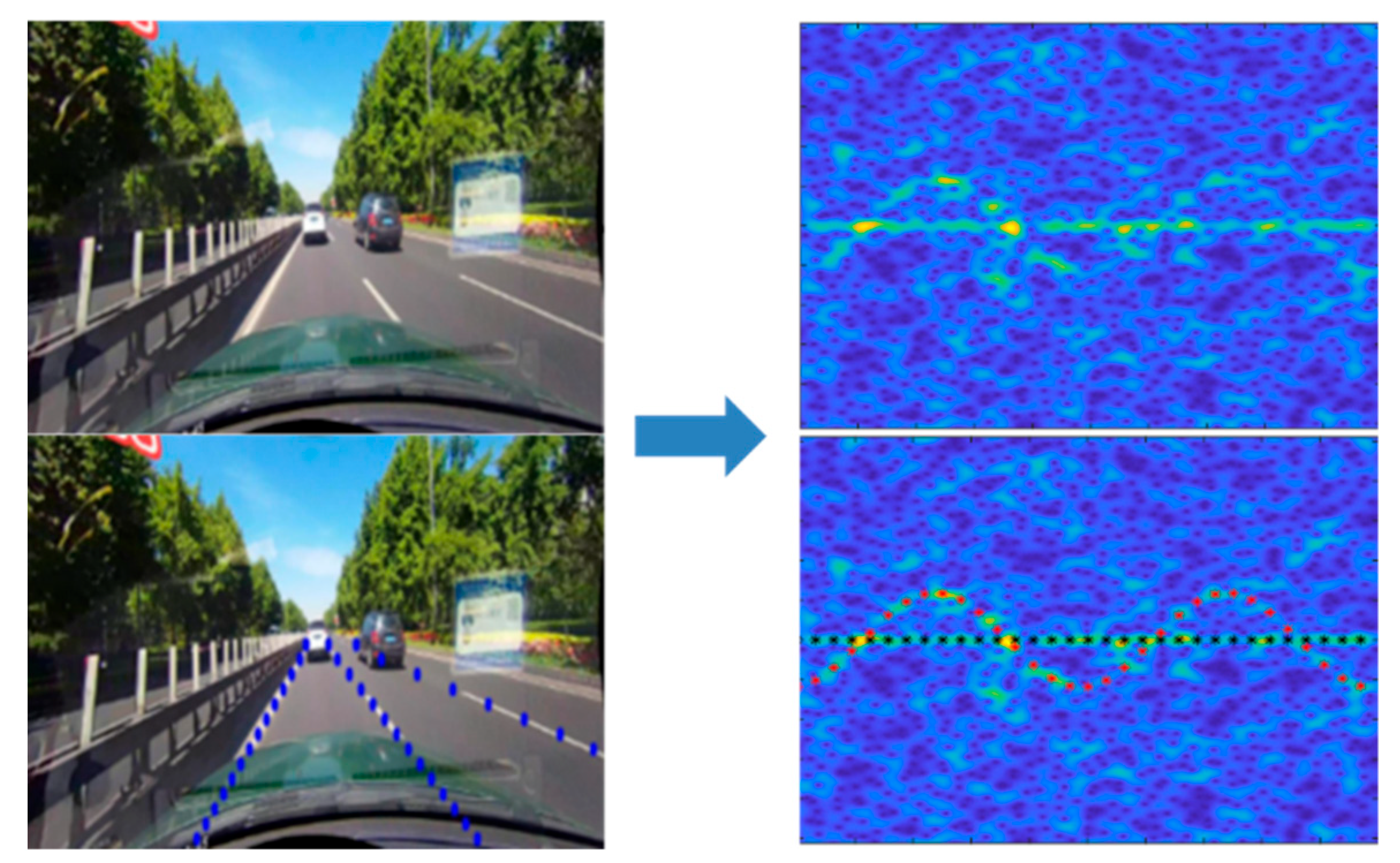
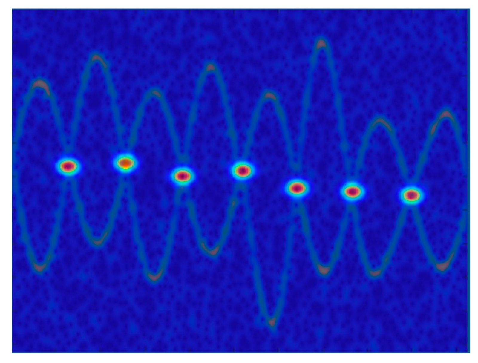
21]. The m-D components with varying instantaneous frequency (IF) can be viewed as semantic lines on the spectrogram, as shown in
Figure 1. Affected by interference such as noise, the signal may be submerged or incomplete but still show continuity in global contexts, which provides the possibility of applying the neural networks to component extraction.
In this paper, we propose a novel and effective dual-branch network-based m-D components extraction method. The contributions of this paper are three-fold.
- (1)
An efficient, dual-branch and multi-task network is proposed to extract the continuous m-D components and their crossing points.
- (2)
The shuffle attention-Fast Fourier convolution (SA-FFC) module is proposed, which can not only fuse the local and global context, but also focus on key information in the channel and space to obtain better performance.
- (3)
A post-processing module to re-group the m-D components to achieve smooth and complete component curves is further designed. The first-order parametric continuous condition and cubic spline interpolation are applied in the module.
2. M-D Signal Model
The micro-motion induces a Doppler modulation on the radar signal, which is referred to as the m-D effect. The m-D reflects the unique dynamic and structural properties of a target and can be used as an important basis for target detection and recognition. For a target with multiple scattering centers, the instantaneous range of the
-th scattering centers to radar is
where
is the distance corresponding to the translation of the target, and
is the distance corresponding to the micro-motion of the
-th scattering center. Therefore, the baseband radar echo of the target can be described as:
where
is the reflectivity of the
-th scattering center, and
is the number of scattering center. The IF of the
-th scattering center is:
where
is the target’s translational Doppler, and
is the m-D of the
-th scattering centers, which can be represented as
is consistent for all scattering centers, while the m-D of each scattering center is different due to the amplitude and initial phase of micro-motion varying for different scattering centers. In general, the extraction of m-D components is referred to as the estimation of the individual m-D or the estimation of the individual radar signal of all scattering centers. In this work, the TFR-based m-D estimation is considered.
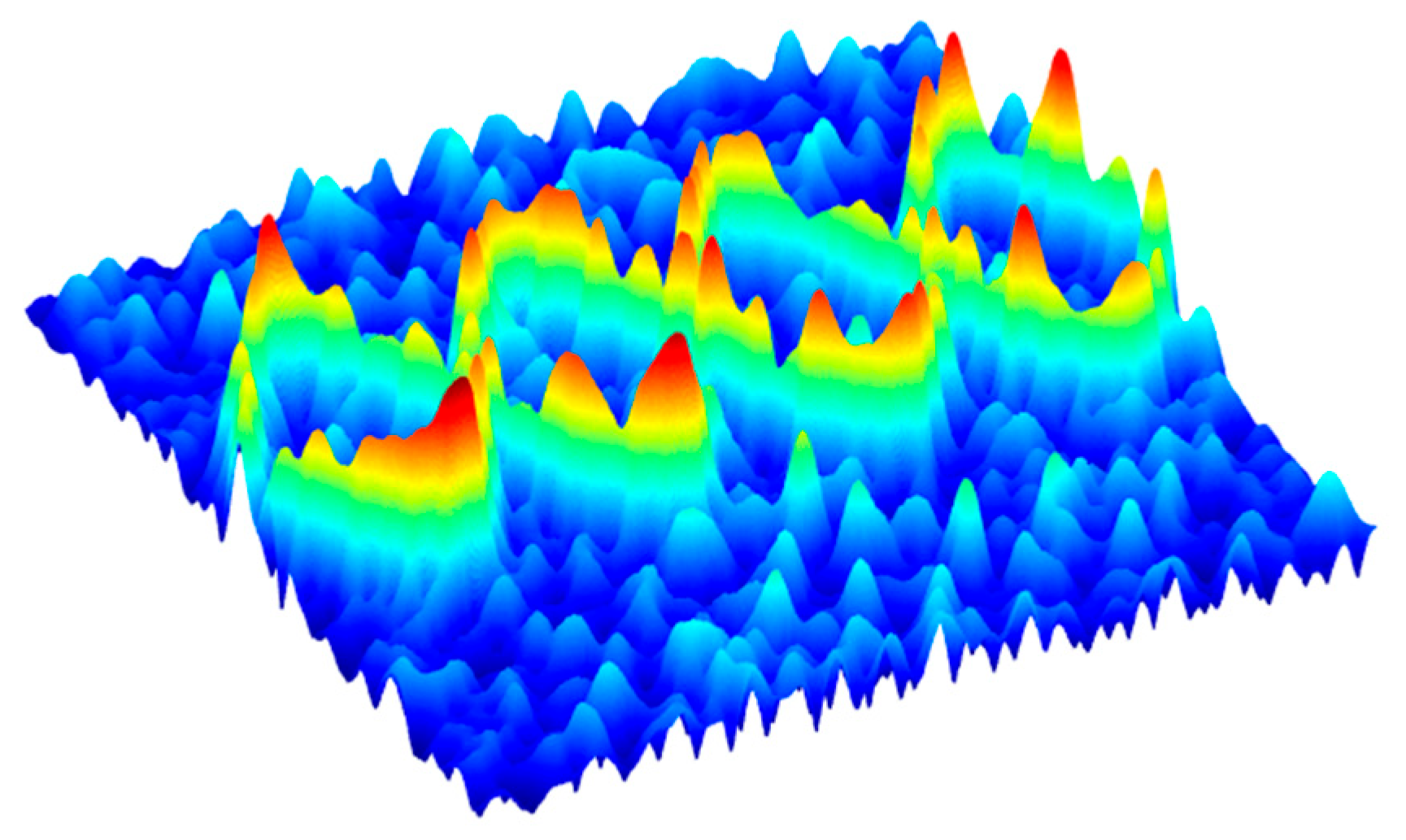
The micro-motion signal can be transformed from the time domain to the time–frequency domain for joint characterization through TFR. As shown in
Figure 2, in the TF plane, the energy of the signal concentrates around the signal’s IFs (m-Ds), which looks like multiple ridges (curves), while the noise distributes over the entire plane [
22].
As one of the most widely used TFR, the short-time Fourier transform (STFT) has the advantages of simple implementation and low computational complexity. The STFT of
can be written as
where
is a symmetric window function. The time–frequency resolution is affected by the length of the window. According to the uncertainty principle of Heisenberg, the time resolution and frequency resolution cannot be optimized at the same time. For the target with multiple scattering points, their m-Ds overlap in the time–frequency plane. Moreover, with the influence of noise or other interference, the signal becomes weak or incomplete. These properties, especially the overlapping m-Ds, makes the extraction of signal components become more challenging.
To deal with the overlapping m-Ds, the TFR-based m-D estimation often contains two processes: extraction of the pixels that belong to the m-D components, and the association of these pixels with the corresponding scattering centers, as shown in
Figure 3. The extraction stage can be peak detection or ridge extraction, while the association is achieved by first finding the continuous parts of the m-Ds and then by connecting the parts before and after intersection points with special features such as slope.
3. Method
As stated in the introduction, the m-D estimation methods have limitations for non-sinusoidal multicomponent m-D signals. In recent years, semantic line detection based on deep learning has developed rapidly and has provided new ideas for signal extraction. The non-sinusoidal signal components in the time–frequency plane can be regarded as semantic lines. With the powerful processing ability of neural networks, the m-D estimation performance can be improved. Below, the principle of neural network-based m-D estimation is presented, followed by the detail of the proposed method.
For a TFR with size , it can be regarded as a set of vectors of time series , is an -dimensional vector. The m-D continuous signal component can be represented by several time series, which is denoted as . is the frequency coordinate of the -th component and presents as a curve in the image.
The m-D estimation process can be expressed as
where function
consists of extraction part
and association part
. The
can be regarded as a map process that converts an
-dimensional vector into a
-dimensional vector, which corresponding the frequency dimension coordinate of components. The task of
is to find the pixels that belong to the m-D components. One can use features such as shape, color and amplitude to achieve this. This task can be transformed to a classification problem and neural network-based segmentation [
23] or anchor-based semantic line detection methods [
20,
24] as shown in
Figure 4. It was proved in [
20] that the anchor-based line detection method has better performance and higher computing efficiency. In view of this, we used this type of method on TFR m-D extraction. At each time instant
, the proposed method outputs
frequency coordinates by using a multilabel classification function, which can be expressed as
After obtaining the estimates for each time instance, component association should be performed. In this work, a two-stage technique for extracting m-D components is proposed. In the first stage, a dual-branch neural network is employed to extract the continuous m-D components (CMDCs) and their crossing points (CPs). The CMDC branch extracts components by employing a column-based selecting method with global characteristics, while the CP branch detects their crossing points by predicting a proposal heatmap. These two branches share the features generated by the backbone network. The backbone adopts the improved ResNet [
25], in which the traditional convolution is replaced with the SA-FFC module proposed in this paper. Compared with the original network, the modified network can realize the fusion of global features and local features.
To further achieve more accurate associations, a post-processing stage is proposed. Since the extracted m-D components of the dual-branch network are represented as sets of positions consisting of multiple fragments, we used the first-order parametric continuity condition to re-link the m-D components and interpolation to generate fine m-D estimation. The overall architecture of the proposed method is shown in
Figure 5.
3.1. SA-FFC ResNet
For targets with long continuous shapes, a wide receptive field is crucial for understanding the whole structure. Compared to conventional convolution, the recently proposed operator fast Fourier convolution (FFC) [
26] has a receptive field that covers the entire image. The FFC fuses local and global contexts through a multi-branch aggregation process.
Specifically, the FFC is comprised of a local branch and a global branch. The input feature maps
are split into a local part and a global part
along channel dimension, and the split ratio is controlled by a hyper-parameter
,
. The split features are input into a local branch and global branch, respectively. The local branch captures local information with vanilla convolution
and
, while the global branch captures the long-range context by performing regular convolution
and spectral transform
. The global and local branch interact with each other via inter-path convolution transition, as illustrated in
Figure 6.
The spectral transform is achieved by the following steps:
Apply real two-dimensional fast Fourier transform (FFT) to the input feature map.
Concatenate the real and imaginary parts of the output of Step 1 together by the channel dimension to convert the output to a real value.
Apply convolution to the output of Step 2.
Split the output of Step 3 across the channel dimension and restore the real value to a complex value.
Apply inverse real two-dimensional FFT to the output of Step 4.
Although multi-scale features which contains sufficient information are obtained, they often contain redundant information, and how to focus on the useful features is another problem. As the two most widely used attention mechanisms, the proposals of spatial attention and channel attention optimize the performance of the network. The shuffle attention (SA) [
27] utilizes the shuffle unit to delineate feature dependencies in spatial and channel dimensions. In this paper, SA is combined with the FFC module. Specifically, the SA module groups the channel dimension of local and global features, respectively, into multiple sub-features, and for each sub-feature the spatial attention and channel attention module are applied in parallel. Specifically, for the output
of the local branch, we divided into
groups sub-features,
. For each sub-feature
, it is spilt into two branches
as the input of spatial attention and channel attention. The spatial and channel attention can be calculated by
where
is global averaging pooling, and
is group normalization. The output of spatial and channel attention are concatenated. The outputs of each sub-feature are aggregated. The information exchange between different sub-features is achieved by operating channel shuffle on fused sub-features.
The SA-FFC can be used as a substitute for regular convolution. In this paper, ResNet was used as the backbone, and the SA-FFC-ResNet could therefore be obtained; the basic block of FFC-SA ResNet is shown in
Figure 7. Assuming the input image size is
I, the size of output feature maps of FFC-ResNet are
,
,
,
, respectively.
3.2. Extraction Stage
3.2.1. CMDC Branch
M-D components can be viewed as a series of vertical locations at each column, and our goal was to distinguish the correct positions of components from the background. Existing lane detection methods are often aimed at lanes that are mostly straight. The situation in this paper was more complicated, as the radar signals were mostly non-sinusoidal curves with overlap. Inspired by the previous work in [
20], a column-based components extraction method was proposed. Compared to segmentation networks, which use the local feature [
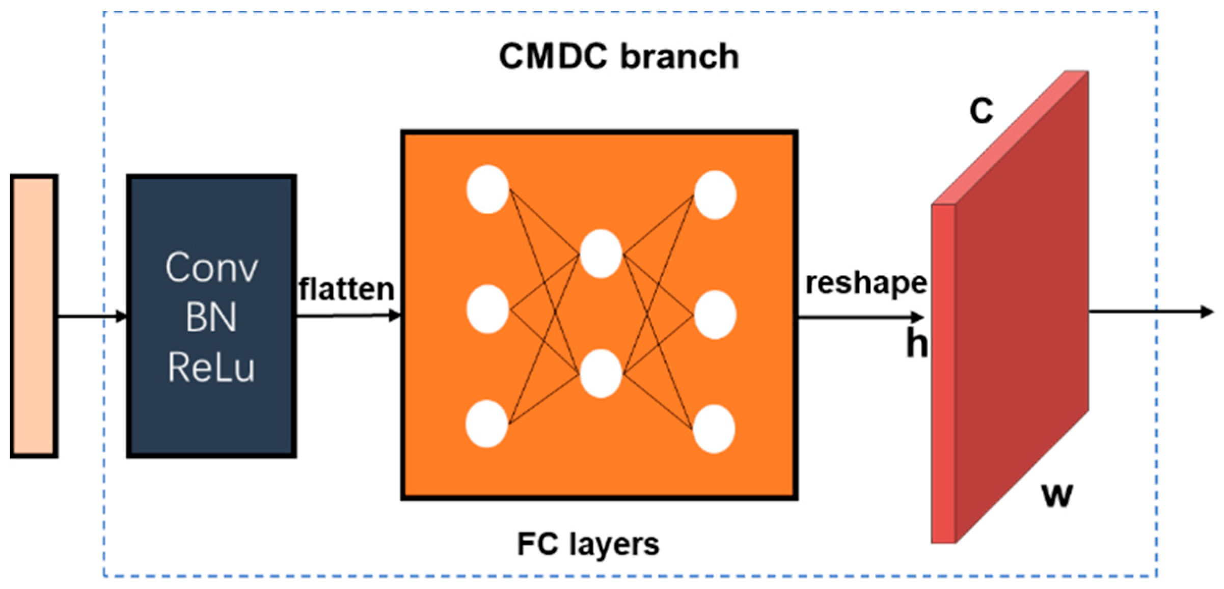
23], the CMDC branch uses the global feature obtained by the FFC-SA Resnet, which can better capture a long continuous shape structure-like component. The structure of the CMDC branch is shown in
Figure 8.
The feature map generated from the backbone, serves as the input of the CMDC branch, with a size of the of the original image. The feature map is compressed by convolution with a kernel to reduce the number of channels. After the compressed feature is obtained, it is flattened and sent to the fully connected (FC) layers, which consist of two layers. The features are flattened before being sent to the FC layers. The FC layers work as a classifier in the entire convolutional neural network, determining whether components exist in divided grids. A dropout operation is embedded in the FC layers, so that it does not rely too much on the local features to prevent overfitting, and the model has stronger generalization performance. Assuming that there are m-D components on the TFR, then the features are restored to by a reshape operation.
As the m-D components occupy a small proportion of the TFR, there is no need for extensive computation to analyze each pixel. To improve computational efficiency, TFR is divided into cells, with each cell corresponding to several pixels. For a TFR with size
, it is divided into grids of shape
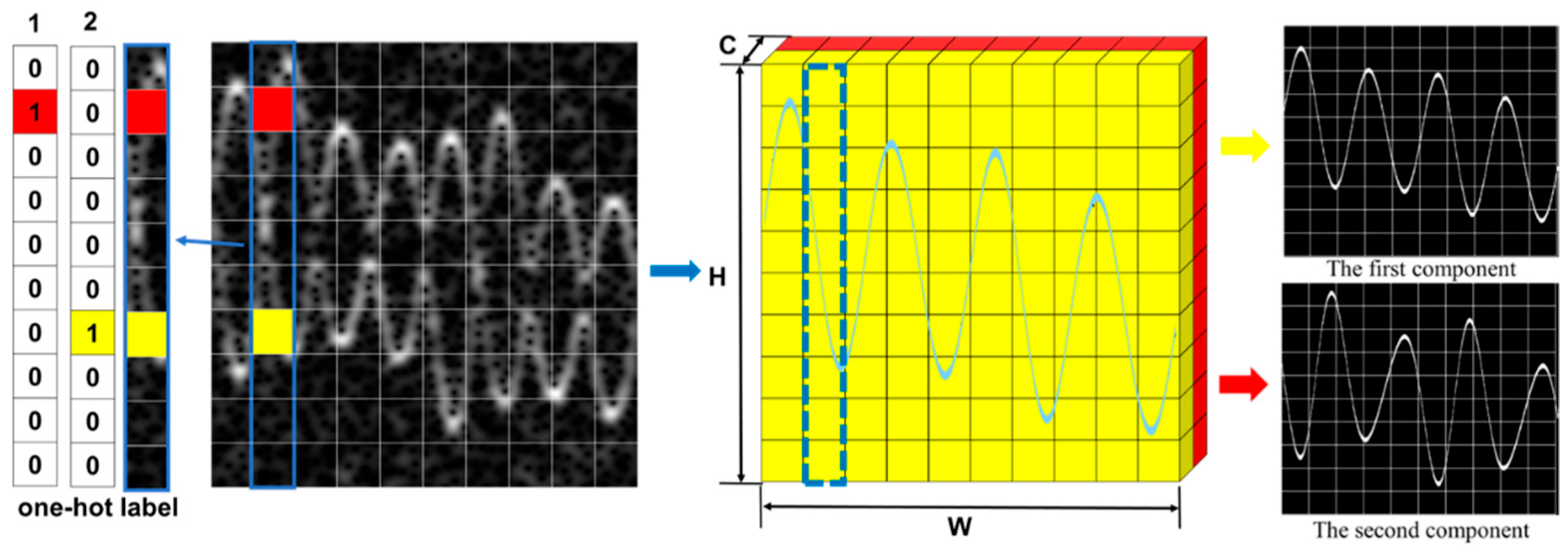
. For each continuous signal component, there is only one label in each column, so the column-based classification method can be used to find the position of the component in each column, as shown in
Figure 9.
For each visual m-D component, its vertical location at each column is estimated based on an
-dimensional probability vector. The output of the CMDC branch is the reshaped classification results. The production of CMDC branch is the position set of all components with size
, which is given by
where
is an
-dimensional vector representing the probability prediction at the
-th column of the
-th m-D component. After obtaining the probabilities, the vertical locations with the highest possibilities in each column are selected.
To alleviate the imbalance of sample distribution, we adopted a standard focal loss to constrain the prediction output
where
is the one-hot label of the correct position of column
. The one-hot label of m-D components is shown in
Figure 9. The focal loss can be written as
where
is predicted value, and the hyper-parameter
is set to 2.
3.2.2. CP Branch
The intersections are relatively small and susceptible to noise, making CP challenging to detect. To find out the crossing points of m-D components, the CP branch inspired by CenterNet [
28] was designed, as shown in
Figure 10.
In this branch, the fusion of high-level semantic features and low-level detail information is applied to detect small targets like CP. Specifically, a feature aggregation-based CP detection method that utilizes multi-scale features to model local features is employed. The backbone network outputs multiple scale features, including high-level semantic features and low-level detail features. Three scale feature maps
,
,
are used in this branch. The feature map
and
are resized to the same size as the feature map
by interpolation. After that, the feature maps are squeezed and concatenated with feature map
across the channel dimension. A heat map reflecting the CP position is generated from the CP branch. The ground truth of heatmap is generated by Gaussian filter to the label map of the CP, as shown in
Figure 11.
Since the number of CPs is small, the modified focal loss in [
28] is adopted as the loss function.
where
is the number of intersections, and
and
are the label and the predicted value of the proposal heatmap at
-th column and
-th row, respectively. Hyper-parameters
and
were set to 2 and 4 in this paper. The branch detects CP effectively by prediction, and the position of CP is therefore obtained.
The multi-task learning is used to train the whole network, i.e., the CMDC branch and CP branch are trained simultaneously. In the training phase, the multi-task loss is defined as follows.
3.3. Post-Processing Stage
Although position sets of m-D components are obtained from the CMDC branch, each set consists of multiple fragments that may belong to different m-D components due to crossing. To further improve the precision of extraction, a post-processing stage consisting of regroup and interpolation operations is conducted to correct the association errors of the previous stage. The post-processing process is shown in
Figure 12.
3.3.1. Regroup
As we obtain the position sets of components and CP, the sets of components can be regrouped around CP obtained from the CP branch, according to the first-order parametric continuous () of components. is a commonly used measure to determine how smoothly a curve transits from one curve segment to another segment, which can be used to determine whether two fragments before and after the junction belong to the same curve.
Since m-D components are represented as a series of vertical locations at predefined columns; the first derivatives are approximated as the slope of lines consisting of positions on adjacent columns. Assuming a CP is between the
-th and
-th column, the slope before and after the CP of the
-th component can then be expressed as
To regroup components, a connection matrix
is designed
The values of the elements in the connection matrix are the absolute values of the difference of the slopes, which are estimated to be less than
. The best combination pair of components can be obtained by finding the minimum element of the connection matrix, which can be represented as
After that, the first elements in the position set of are combined with the last elements in the position set of . To regroup other components, the elements in the -th row and the -th column of are set to . Then the above process is repeated until we find pairs. The procedure is repeated for each CP.
3.3.2. Interpolation
Since the components are extracted on the down-sampled locations, we interpolate the regrouped set to generate smooth component curves in the origin spectrogram. A univariate cubic spline interpolation [
29] is applied to fit curves to the provided sets. The number of knots can be specified to control the degree of curve smoothness.
4. Numerical Results
To evaluate the proposed approach, we performed experiments on simulated scenarios and measured data. The data used in the simulation scenario were generated by the model established in the M-D signal model section. The measured signal data were collected by a millimeter-wave radar.
4.1. Simulation Experiment Setup
4.1.1. Dataset
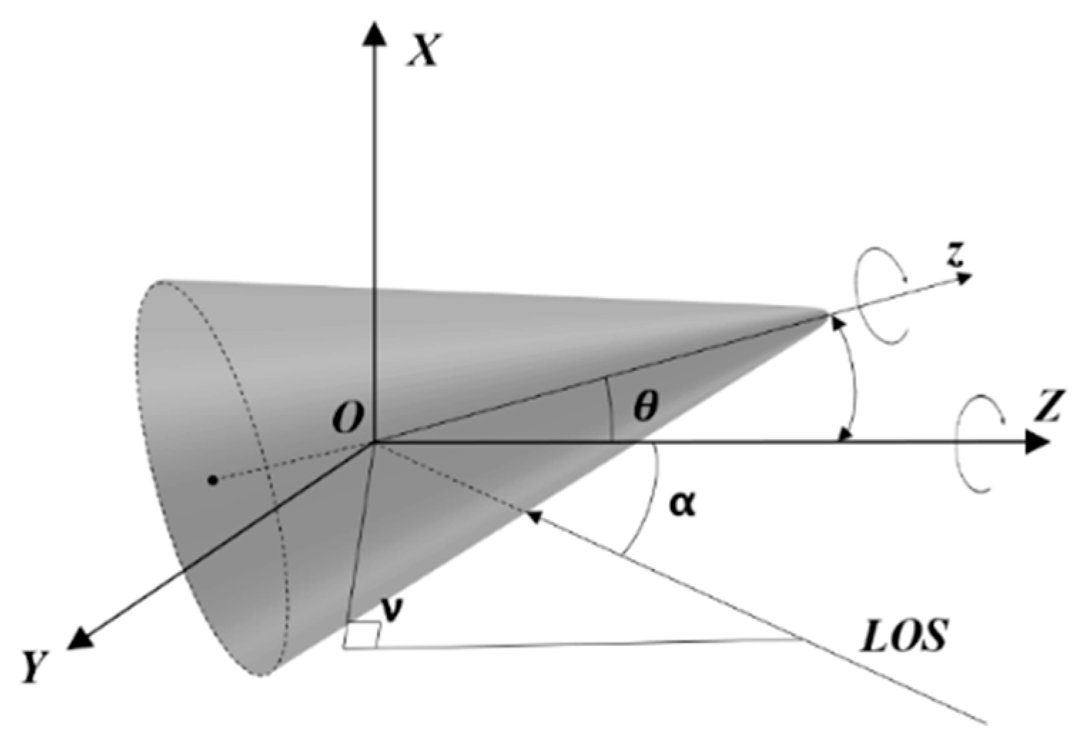
As a typical multi-scatter target, a cone-shape target is widely used to model ballistic targets with micro-motion (The proposed method is model agnostic. The cone model is taken as an example, and the trainset is generated by this model). For simplicity and convenient analysis, a cone-shape target was considered in this paper. The reference coordinates system
and the target local coordinate system
were established with the center of mass as the coordinate origin
, as shown in
Figure 13.
is the azimuth of radar line of sight (LOS) at the reference coordinate system. The angle between LOS and Z was set to
.
For the
-th point scatterer on the target, the instantaneous range to the radar could be expressed as
where
is the range corresponding to the target translation,
is the initial position of the scatterer in local coordinate and
is the initial rotation matrix that represents the initial attitude of the target.
,
and
are the rotation matrixes of oscillating, coning and spinning motion, respectively, and
is the unit direction vector of radar line of sight. The specific derivation can be obtained in [
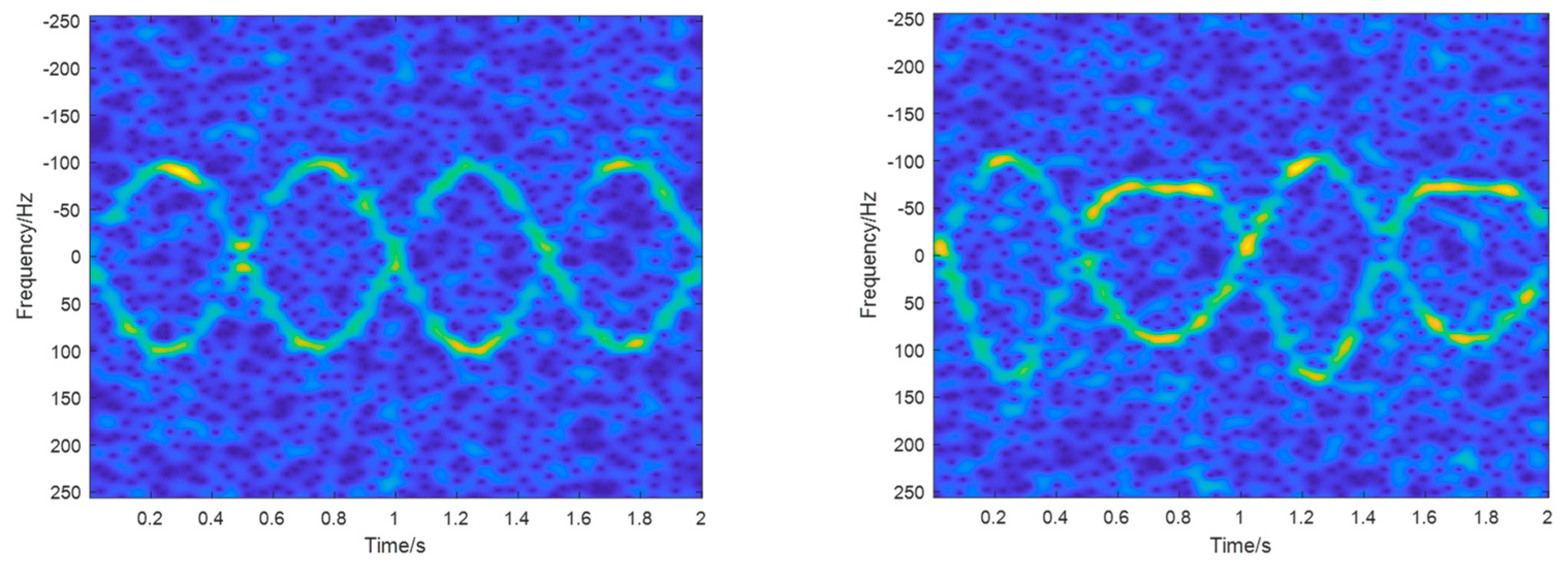
30]. Due to the cone-shaped target being rotationally symmetrical, the spinning has no modulated effect on the scattering characteristics of electromagnetic waves. The precession is the combination of coning and spinning, while the nutation is the combination of precession and oscillating.
Figure 14 shows TFR of precession and nutation without translation. The time–frequency curves of precession appeared to be sinusoidal, while the time–frequency curves of nutation had obvious distortion. Affected by noise, the curve appeared discontinuous, but it still had a strong shape prior and global context information, which enabled the neural network to capture its global continuity.
We assumed that the radar operated at 10 GHz, and the pulse repetition frequency (PRF) was 1024 Hz. Gaussian white noise was added, with the signal-noise ratio (SNR) between dB randomly. To make the simulation more realistic, a translation was added to the target. The translation was . A Hamming window with a length of 65 was employed in the computation of STFT.
The observation time was set to
s. This paper mainly considered precession and nutation. In addition to the case where there was only one motion, we considered a more complex case where the state of motion changed. In this case, the precession became nutation after
s. The settings of simulation parameters are listed in
Table 1. For simplicity and convenient analysis, we chose two strong effective scatterer points whose positions were
m and
m to simulate the radar signal model. We assumed each point scatterer had the same scattering intensity. With comprehensive consideration of computing efficiency and accuracy, we set
and
for training, respectively.
It is worth mentioning that although the data set was established based on the cone model, the method proposed in this paper is not limited to the model and motion form and has good generalization.
4.1.2. Implementation Details
The experiment was conducted with PyTorch on Tesla V100 GPUs. The input size of TFR was 512 × 512. All models were trained for 40 epochs with a batch size of 16. An Adam optimizer with cosine decay learning rate strategy was applied to train our model. The initial value of the learning rate was 0.01.
To improve the performance of network generalization, a data augmentation operation was conducted. In each iteration, we randomly chose augmentation operations from resize, crop, flip horizontally or vertically and spatial shift.
4.1.3. Evaluation Metrics
The evaluation metrics of the CULane dataset [
31] and TuSimple dataset [
32] were introduced in this paper, which were referred to as the F1 metric and accuracy metric.
For the F1 metric, the components in TFR were viewed as curvilinear targets with widths equal to 20 pixels. The true positives (TP) were components whose intersection-over-union (IoU) between the ground truth and the prediction was larger than a certain threshold. The
and
could therefore be obtained. The F1-measure could be calculated as
In this paper, we set 0.5 and 0.7 thresholds corresponding to loose and strict evaluations. By comparing the F1 scores of different settings, the effectiveness of the post-processing stage could be verified.
The accuracy metric was obtained by calculating the ratio of the number of correctly predicted points to the number of all points, which was calculated by
in which
is the number of points predicted correctly, and
is the total number of ground truths in each clip.
Apart from the evaluation metrics mentioned above, we further quantitatively analyzed the performance by computing root mean square error (RMSE) between the estimated IF and the original IF. The RMSE is represented as
where
are the true instantaneous frequencies of the signal and
are the estimated instantaneous frequencies,
is the discrete time and the superscript
represents the
-th simulation.
4.2. Results and Analysis
4.2.1. Effectiveness of the Proposed Method
Firstly, we verified the effectiveness of the proposed methods. A total of 800 simulations were generated randomly according to the parameters in
Table 1 for SNR varying from −5 to 15 dB. The baseline stands for Resnet-50 with vanilla conventional convolution. As we can see from
Table 2, the post-processing stage brought out improvement in F1 scores by correcting false associations. Baseline stands for Resnet-50 with vanilla convolution. As we can see, the FFC module brought a slight improvement in performance, while the accuracy and F1 score of the SA-FFC module increased by 0.93% and 1.13, respectively. The post-processing modules brought further improvements to performance. The proposed method finally brought 1.33% and 1.51 improvement in accuracy and F1 score, respectively. The validity of the combination of the SA-FFC module and post-processing was verified.
We further analyzed the network performance from the amount of parameters and complexity by conducting quantitative experiments. As shown in
Table 3, the experiments were carried out with the same training settings and different module combinations. The SE in the table represents the squeeze-and-excitation block. As we can see, the performance of the proposed module surpassed the original backbone. With less complexity, the performance of the proposed module was comparable to FFC SE ResNet-50, which proved the effectiveness of the proposed modules.
4.2.2. Comparison with Traditional Methods
To further demonstrate the effectiveness of the proposed method, we compared it with several commonly used component extraction methods: RPRG [
12], VA [
11] and ADTFD-RT [
13]. The F1 score, accuracy and running time on the test dataset mentioned above are listed in
Table 4. The comparison algorithm was based on MATLAB with an R7-4800H CPU, while the proposed method was based on PyTorch with a Tesla V100 GPU. The running time was the average time of simulations.
It was shown that with the use of GPU, the proposed method had the least computation time. Though other methods may have the possibility to be accelerated by GPU, there is still much effort to rebuild them, which is not available currently.
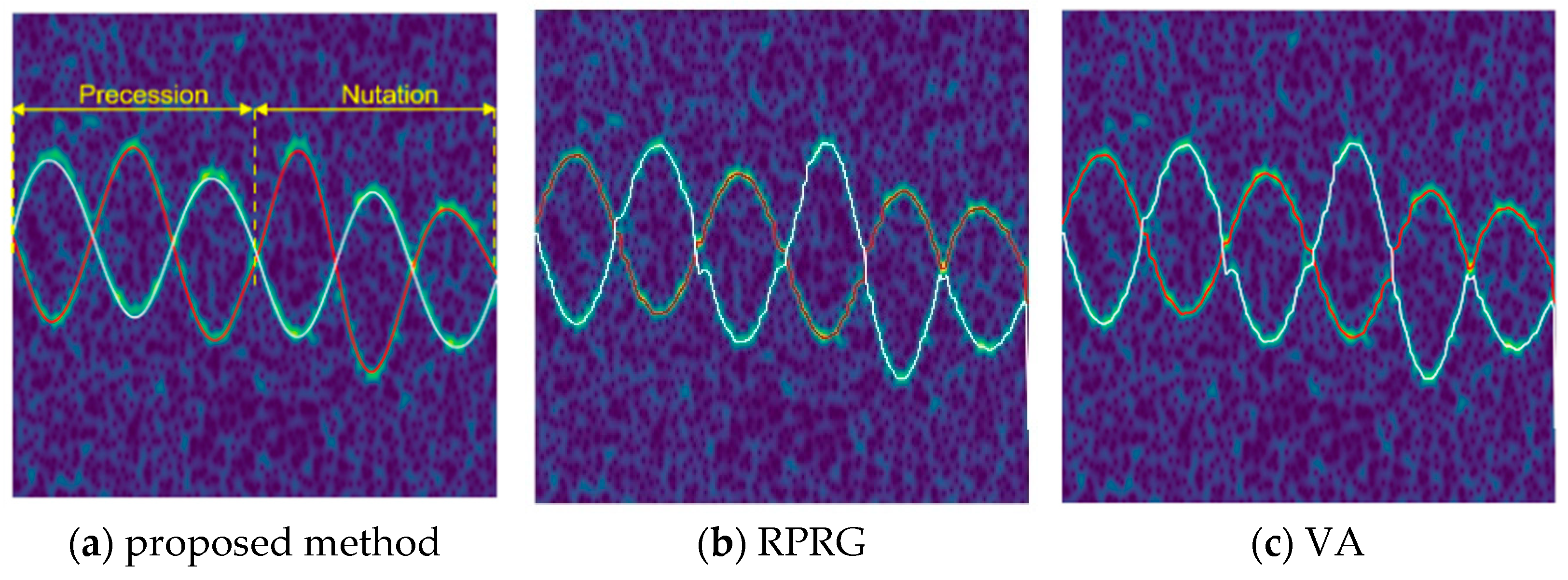
Figure 15 shows the visualization results of the proposed method along with the RPRG and VA. The proposed method could effectively extract the m-D components with CP, while the performance of RPRG was affected by the quality of the detected ridge curves. VA still had the switch problem at CP, as shown in
Figure 15c.
The curves in TFR corresponded to the instantaneous frequencies of the target’s scattering centers. We further quantitatively analyzed the performance of the proposed method with the VA, ADTFD-RT and RPRG by computing root mean square error (RMSE). In total, 100 simulations, the parameters of which were selected randomly from
Table 1, were performed for each SNR, varying from −5 to 15 dB.
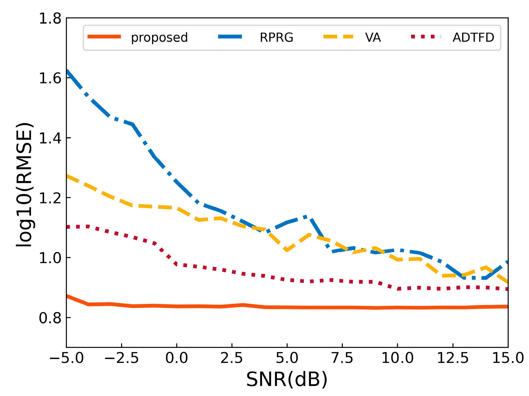
As is shown in
Figure 16, the RMSE of VA and RPRG decreased significantly with the increase of SNR, while the proposed method was hardly affected by SNR. The ADTFD-RT extracts signal components by recursive filtering the strongest components based on adaptive directional time–frequency distribution, but the repetitive computation of ADTFD is computationally expensive. The figure indicates that the proposed method achieved the best performance for non-sinusoidal components. The RMSE of the proposed method was less than 1 Hz for all SNR levels.
4.2.3. Effects of Size of Grid and
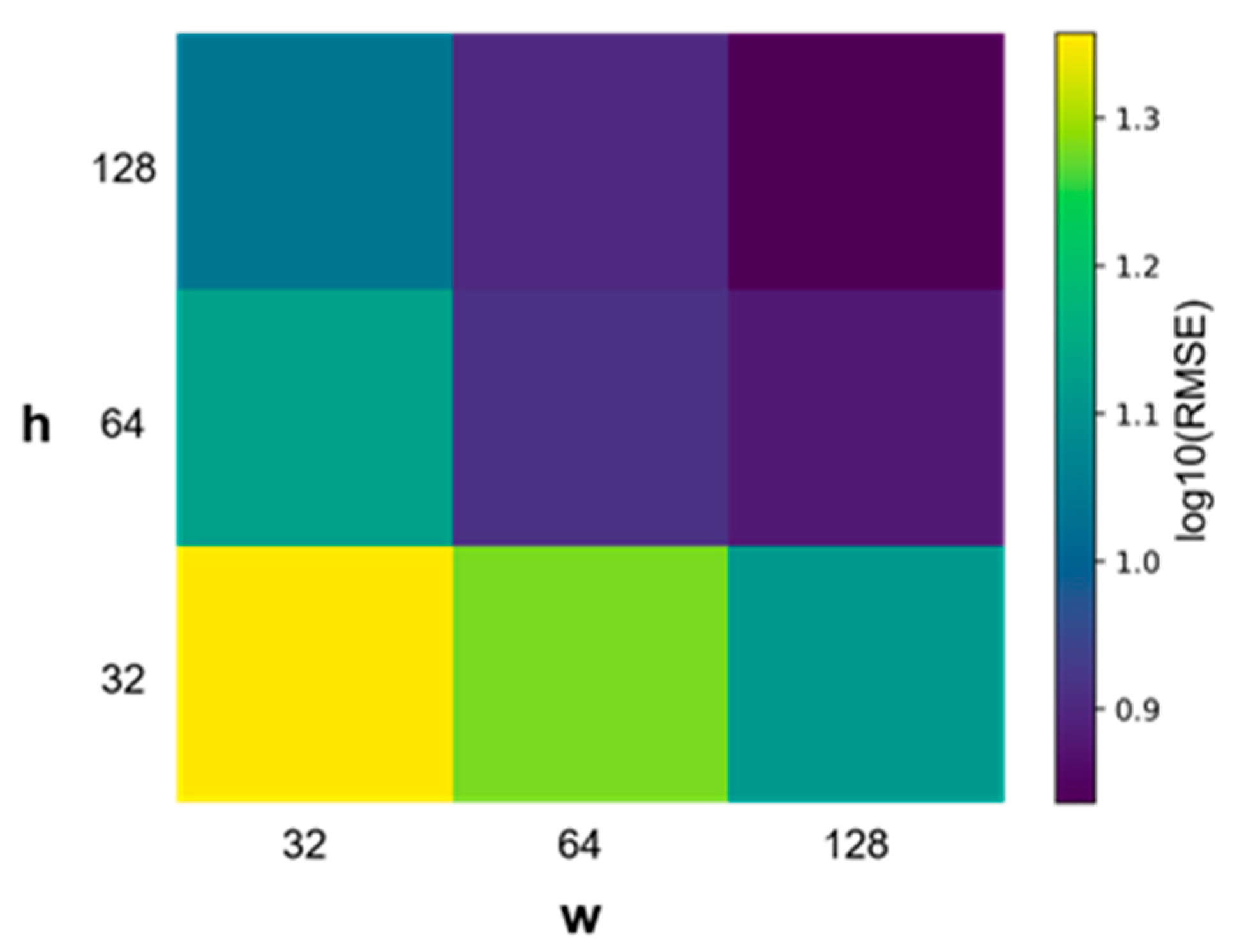
The influence of the size of the grid on the results was analyzed as shown in
Figure 17. With the increase of
and
, cells became smaller, so location was more precise, which consequently resulted in a decrease of the RMSE. However, more gridding cells means a more complex classification is required, and the computational costs increase accordingly. There is no significant improvement when the number of grids is greater than
.
4.2.4. Experiment with Measured Radar Data
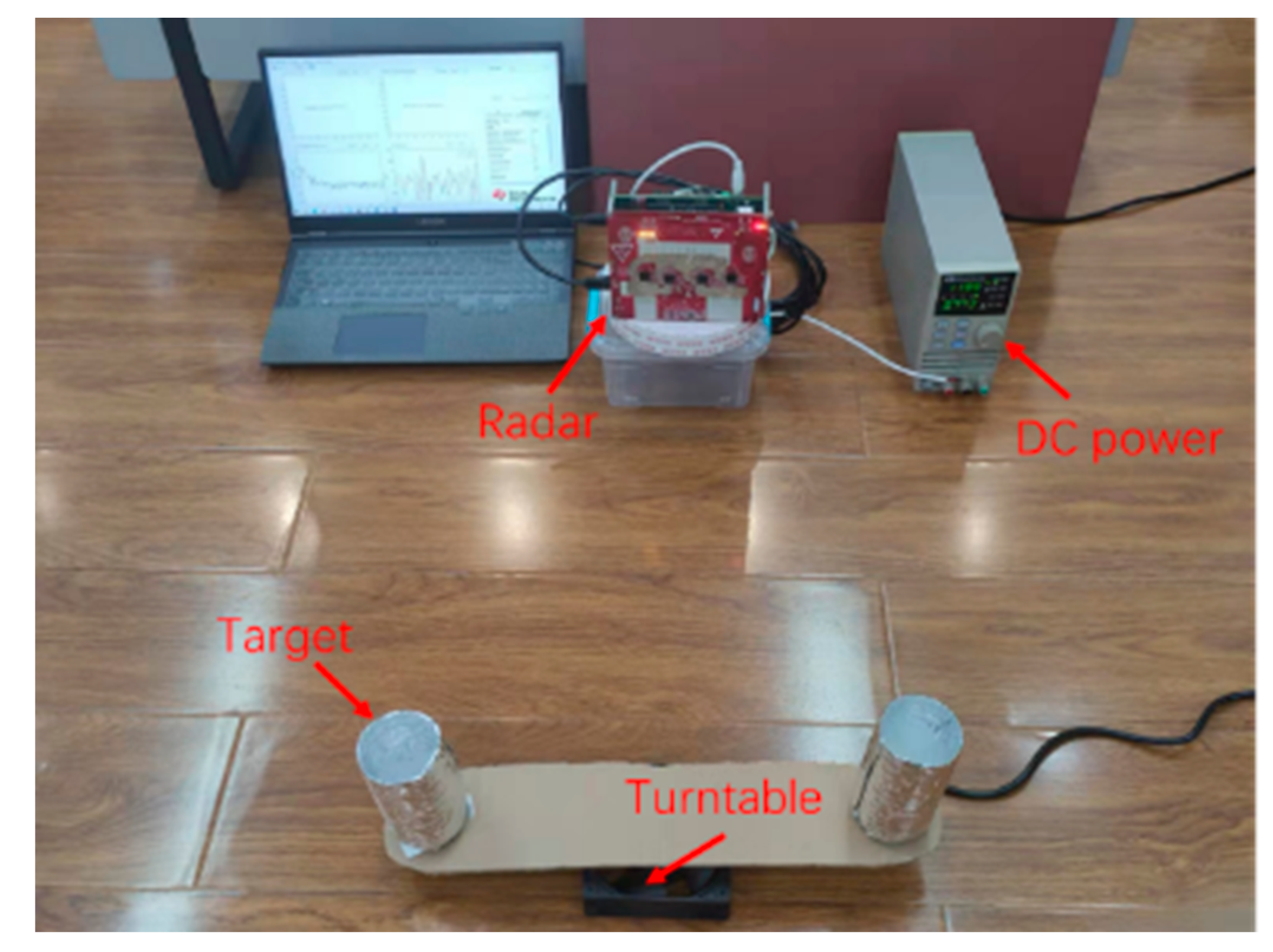
In order to further verify the effectiveness of the proposed method, we presented an experiment with measured radar data. The experimental setup is shown in
Figure 18. A frequency modulated continuous wave (FMCW) radar was used to collect the target echo. The parameter settings of the radar are listed in
Table 5. Two cylindrical targets covered with aluminum foil were placed on either side of the turntable, rotating around the same center of rotation. The m-D signal obtained by two targets was analyzed.
The TFR of the obtained m-D signal appeared as sinusoidal curves when the turntable rotated at a constant speed. When the turntable started/stopped suddenly or changed its motion state, non-uniform rotation occurred, resulting in an irregular non-sinusoidal m-D signal. When the turntable started suddenly, the turntable accelerated, and we acquired two non-sinusoidal m-D signal segments.
The amplitude of m-D increased gradually with the period decreasing gradually in the first segment, while the amplitude and period of m-D changed gently in the second segment. Affected by the uneven surface of the target, the scattering intensity was unevenly distributed and varied periodically. The model trained on simulation data was transferred directly to extract components of the measured data, and the variation of the time–frequency curve of the collected data was not included in the simulation data set. As the result in
Figure 19 shows, the proposed method could effectively extract the cross components in the TFR. Even if the signal was fuzzy, weak, or incomplete due to noise or other interference, it could be extracted by the strong processing ability of the neural network. The proposed algorithm’s validity and superiority were proven in these experiments.
5. Discussion
The estimation of the m-Ds is of great importance. By estimating m-Ds, the exact state of the target and the components of it can be obtained, which is helpful for the subsequent recognition and classification. In this paper, we conducted experiments based on a cone-shaped model for simplicity, although the proposed method can apply to any model. There are three kinds of evaluation metrics that were applied to the experiment. The effectiveness of each module was proven, and the computational complexity and precision of the network were further studied.
In the case of low SNR, the performance of the proposed algorithm degraded, which is consistent with existing research findings. However, compared with the previous research, the SNR had less interference on the proposed method, which reflects its robustness and effectiveness. By making use of global features and contextual information, the method in this paper achieved better m-D estimation performance, while existing methods only utilize local and adjacent features to achieve extraction and association processes. The performance is further improved by quadratic association in the post-processing module.
We only discuss a simple case of the double-scattering point model in this paper. It should be pointed out that the performance of the proposed method will be degraded when it is applied to more complex cases where the m-D signal curves are discontinuous or experience strong signal interference due to clutter as they raise new problems. To deal with this case, it is suggested to incorporate novel modules that can deal with these new cases. Moreover, since this method is a data-driven method, to ensure the generalization of the model, abundant annotated data are required, which are difficult to obtain in real life. How to achieve m-Ds estimation in a small sample or unsupervised situations will be a future research direction.
6. Conclusions
Unlike most prevailing radar applications such as radar target recognition and detection, this paper is a new attempt to apply neural networks to radar signal processing. A method combining a dual-branch network and post-processing is proposed to extract crossing non-sinusoidal micro-Doppler components. The network backbone with an SA-FFC module can exploit global and multi-scale features that output good features for later processing modules, while the CMDC and CP branch can achieve fast, stable and effective extraction of m-D components and cross points. The post-processing regroups and interpolate the extracted components and further improves the performance. The accuracy and F1 score reach 97.5% and 89.1%, respectively. Experiments using simulation and measured data validate the generalization and effectiveness of the proposed method. This paper mainly demonstrate the performance of the two-component m-D signal. Further research on how to achieve extraction on a more sophisticated signal will be carried out.
Author Contributions
Conceptualization, W.Z.; Data curation, W.Y.; Funding acquisition, Y.L.; Investigation, J.L.; Methodology, J.L.; Software, J.L.; Supervision, W.Z. and Y.L.; Validation, Y.L.; Writing—original draft, J.L.; Writing—review and editing, W.Z. All authors have read and agreed to the published version of the manuscript.
Funding
This work was funded by the National Natural Science Foundation of China under Grants 61901487, 61871384 and 61921001; the Natural Science Foundation of Hunan Province under Grant 2021JJ40699; and the China Postdoctoral Science Foundation under Grant 2021TQ0084.
Data Availability Statement
Not applicable.
Conflicts of Interest
The authors declare no conflict of interest.
References
- Chen, V.C.; Li, F.; Ho, S.-S.; Wechsler, H. Micro-Doppler effect in radar: Phenomenon, model, and simulation study. IEEE Trans. Aerosp. Electron. Syst. 2006, 42, 2–21. [Google Scholar] [CrossRef]
- Zhou, Y.; Chen, Z.; Zhang, L.; Xiao, J. Micro-Doppler Curves Extraction and Parameters Estimation for Cone-Shaped Target With Occlusion Effect. IEEE Sens. J. 2018, 18, 2892–2902. [Google Scholar] [CrossRef]
- Li, Y.; Xia, W.; Dong, S. Time-based multi-component irregular FM micro-Doppler signals decomposition via STVMD. IET Radar Sonar Navig. 2020, 14, 1502–1511. [Google Scholar] [CrossRef]
- Hanif, A.; Muaz, M.; Hasan, A.; Adeel, M. Micro-Doppler Based Target Recognition With Radars: A Review. IEEE Sens. J. 2022, 22, 2948–2961. [Google Scholar] [CrossRef]
- Zhao, Y.; Su, Y. The Extraction of Micro-Doppler Signal With EMD Algorithm for Radar-Based Small UAVs’ Detection. IEEE Trans. Instrum. Meas. 2020, 69, 929–940. [Google Scholar] [CrossRef]
- Mohanty, S.; Gupta, K.K.; Raju, K.S. Hurst based vibro-acoustic feature extraction of bearing using EMD and VMD. Measurement 2018, 117, 200–220. [Google Scholar] [CrossRef]
- Zhu, L.; Zhao, H.; Xu, H.; Lu, X.; Chen, S.; Zhang, S. Classification of Ground Vehicles Based on Micro-Doppler Effect and Singular Value Decomposition. In Proceedings of the 2019 IEEE Radar Conference (RadarConf), Boston, MA, USA, 22–26 April 2019; pp. 1–6. [Google Scholar]
- Li, Y.; Li, P. Ballistic Target Signal Separation Based on Fast Independent Component Analysis Algorithm. In Proceedings of the 2021 International Symposium on Computer Technology and Information Science (ISCTIS), Guilin, China, 4–6 June 2021; pp. 320–323. [Google Scholar]
- Zhou, Y.; Bi, D.; Shen, A.; Wang, X. Hough transform-based large micro-motion target detection and estimation in synthetic aperture radar. IET Radar Sonar Navig. 2019, 13, 558–565. [Google Scholar] [CrossRef]
- Sathe, P.; Dyana, A.; Ray, K.P.; Shashikiran, D.; Vengadarajan, A. Helicopter Main and Tail Rotor Blade Parameter Extraction Using Micro-Doppler. In Proceedings of the 2018 19th International Radar Symposium (IRS), Bonn, Germany, 20–22 June 2018; pp. 1–10. [Google Scholar]
- Li, P.; Zhang, Q.-H. IF Estimation of Overlapped Multicomponent Signals Based on Viterbi Algorithm. Circuits Syst. Signal Process. 2020, 39, 3105–3124. [Google Scholar] [CrossRef]
- Chen, S.; Dong, X.; Xing, G.; Peng, Z.; Zhang, W.; Meng, G. Separation of Overlapped Non-Stationary Signals by Ridge Path Regrouping and Intrinsic Chirp Component Decomposition. IEEE Sens. J. 2017, 17, 5994–6005. [Google Scholar] [CrossRef]
- Khan, N.A.; Mohammadi, M.; Ali, S. Instantaneous frequency estimation of intersecting and close multi-component signals with varying amplitudes. Signal Image Video Process. 2019, 13, 517–524. [Google Scholar] [CrossRef]
- Zhu, X.; Zhang, Z.; Gao, J. Three-dimension extracting transform. Signal Process. 2021, 179, 107830. [Google Scholar] [CrossRef]
- Zhu, X.; Yang, H.; Zhang, Z.; Gao, J.; Liu, N. Frequency-chirprate reassignment. Digit. Signal Process. 2020, 104, 102783. [Google Scholar] [CrossRef]
- Zhang, R.; Cao, S. Real-Time Human Motion Behavior Detection via CNN Using mmWave Radar. IEEE Sens. Lett. 2019, 3, 1–4. [Google Scholar] [CrossRef]
- Tan, M.; Zhou, J.; Xu, K.; Peng, Z.; Ma, Z. Static Hand Gesture Recognition With Electromagnetic Scattered Field via Complex Attention Convolutional Neural Network. IEEE Antennas Wirel. Propag. Lett. 2020, 19, 705–709. [Google Scholar] [CrossRef]
- Li, R.; Zhang, S.; Zhang, C.; Liu, Y.; Li, X. Deep Learning Approach for Sparse Aperture ISAR Imaging and Autofocusing Based on Complex-Valued ADMM-Net. IEEE Sens. J. 2021, 21, 3437–3451. [Google Scholar] [CrossRef]
- Zhao, K.; Han, Q.; Zhang, C.-B.; Xu, J.; Cheng, M.-M. Deep hough transform for semantic line detection. IEEE Trans. Pattern Anal. Mach. Intell. 2021, 44, 4793–4806. [Google Scholar] [CrossRef]
- Qin, Z.; Wang, H.; Li, X. Ultra fast structure-aware deep lane detection. In Proceedings of the Computer Vision–ECCV 2020: 16th European Conference, Glasgow, UK, 23–28 August 2020; pp. 276–291. [Google Scholar]
- Rubio Perona, F.; Flores Gallego, M.J.; Puerta Callejón, J.M.J.E. An Application for Aesthetic Quality Assessment in Photography with Interpretability Features. Entropy 2021, 23, 1389. [Google Scholar] [CrossRef]
- Khan, N.A.; Djurović, I. ADTFD-RANSAC For multi-component IF estimation. Signal Process. 2022, 195, 108494. [Google Scholar] [CrossRef]
- Neven, D.; De Brabandere, B.; Georgoulis, S.; Proesmans, M.; Van Gool, L. Towards end-to-end lane detection: An instance segmentation approach. In Proceedings of the 2018 IEEE Intelligent Vehicles Symposium (IV), Changshu, China, 26–30 June 2018; pp. 286–291. [Google Scholar]
- Qin, Z.; Zhang, P.; Li, X. Ultra Fast Deep Lane Detection With Hybrid Anchor Driven Ordinal Classification. IEEE Trans. Pattern Anal. Mach. Intell. 2022. [Google Scholar] [CrossRef]
- He, K.; Zhang, X.; Ren, S.; Sun, J. Deep residual learning for image recognition. In Proceedings of the IEEE Conference on Computer Vision and Pattern Recognition, Las Vegas, NV, USA, 27–30 June 2016; pp. 770–778. [Google Scholar]
- Chi, L.; Jiang, B.; Mu, Y. Fast Fourier Convolution. In Proceedings of the NeurIPS, Virtual, 6–12 December 2020. [Google Scholar]
- Zhang, Q.-L.; Yang, Y.-B. Sa-net: Shuffle attention for deep convolutional neural networks. In Proceedings of the ICASSP 2021–2021 IEEE International Conference on Acoustics, Speech and Signal Processing (ICASSP), Toronto, ON, Canada, 6–11 June 2021; pp. 2235–2239. [Google Scholar]
- Zhou, X.; Wang, D.; Krähenbühl, P.J.A. Objects as Points. arXiv 2019, arXiv:1904.07850. [Google Scholar]
- Dierckx, P. Curve and surface fitting with splines. In Monographs on Numerical Analysis; Oxford University Press: Oxford, UK, 1996. [Google Scholar]
- Gao, H.; Xie, L.; Wen, S.; Kuang, Y. Micro-Doppler Signature Extraction from Ballistic Target with Micro-Motions. IEEE Trans. Aerosp. Electron. Syst. 2010, 46, 1969–1982. [Google Scholar] [CrossRef]
- Pan, X.; Shi, J.; Luo, P.; Wang, X.; Tang, X. Spatial as deep: Spatial cnn for traffic scene understanding. In Proceedings of the Proceedings of the AAAI Conference on Artificial Intelligence, Edmonton, AB, Canada, 13–17 November 2018. [Google Scholar]
- TuSimple. Tusimple Benchmark. Available online: https://github.com/TuSimple/ (accessed on 22 October 2019).
Figure 1.
Semantic line detection and radar signal extraction.
Figure 1.
Semantic line detection and radar signal extraction.
Figure 2.
TFR of micro-Doppler signals.
Figure 2.
TFR of micro-Doppler signals.
Figure 3.
Extraction and Association Process.
Figure 3.
Extraction and Association Process.
Figure 4.
Problem transformation.
Figure 4.
Problem transformation.
Figure 5.
Overview of the proposed method.
Figure 5.
Overview of the proposed method.
Figure 6.
An overview of the proposed SA-FFC module.
Figure 6.
An overview of the proposed SA-FFC module.
Figure 7.
The basic block of FFC-SA ResNet.
Figure 7.
The basic block of FFC-SA ResNet.
Figure 8.
The structure of the CMDC branch.
Figure 8.
The structure of the CMDC branch.
Figure 9.
Column-based classification of a two-component m-D signal.
Figure 9.
Column-based classification of a two-component m-D signal.
Figure 10.
The structure of the CP branch.
Figure 10.
The structure of the CP branch.
Figure 11.
Heatmap of cross points.
Figure 11.
Heatmap of cross points.
Figure 12.
Schematic of post-processing. (a) Extracted components and cross points. (b) Regrouped and interpolated components.
Figure 12.
Schematic of post-processing. (a) Extracted components and cross points. (b) Regrouped and interpolated components.
Figure 13.
Geometry of the cone-shaped target.
Figure 13.
Geometry of the cone-shaped target.
Figure 14.
TFR of precession and nutation.
Figure 14.
TFR of precession and nutation.
Figure 15.
Extraction results of the proposed method, RPRG and VA.
Figure 15.
Extraction results of the proposed method, RPRG and VA.
Figure 16.
Comparison results of RMSE versus SNR.
Figure 16.
Comparison results of RMSE versus SNR.
Figure 17.
Performance under the different sizes of grids.
Figure 17.
Performance under the different sizes of grids.
Figure 18.
The experimental setup.
Figure 18.
The experimental setup.
Figure 19.
Measured data and results.
Figure 19.
Measured data and results.
Table 1.
Parameters of simulation.
Table 1.
Parameters of simulation.
| Target Height (m) | 2 | Bottom Radius (m) | 0.2 |
| Precession frequency (Hz) | 0.8:0.2:2 | Precession angle (°) | 10:1:15 |
| Nutation frequency (Hz) | 0.7:0.1:1 | Nutation angle (°) | 3:1:6 |
| 30:4:70 | | 270 |
Table 2.
Effectiveness of the proposed module.
Table 2.
Effectiveness of the proposed module.
| Baseline | FFC | SA | Post-Processing | F1 (0.7) | Accuracy (%) |
|---|
| ✓ | | | | 87.62 | 96.20 |
| ✓ | ✓ | | | 87.65 | 96.38 |
| ✓ | ✓ | ✓ | | 88.75 | 97.13 |
| ✓ | ✓ | ✓ | ✓ | 89.13 | 97.53 |
Table 3.
Experimental results with different backbone.
Table 3.
Experimental results with different backbone.
| Backbones | F1 (0.5) | F1 (0.7) | Accuracy (%) | Params (M) | GFLOPs |
|---|
| ResNet-50 | 95.37 | 87.62 | 96.20 | 282.34 | 41.13 |
| SE ResNet-50 | 95.50 | 87.87 | 96.96 | 284.85 | 41.16 |
| SA ResNet-50 | 95.37 | 87.62 | 96.95 | 282.34 | 41.14 |
| FFC ResNet-50 | 95.50 | 87.65 | 96.38 | 286.96 | 43.55 |
| SE- FFC ResNet-50 | 96.50 | 88.75 | 97.17 | 290.02 | 43.59 |
| SA- FFC ResNet-50 | 96.50 | 88.75 | 97.13 | 286.96 | 43.57 |
Table 4.
Experimental results of different methods.
Table 4.
Experimental results of different methods.
| Methods | Proposed Method | RPRG | VA | ADTFD-RT |
|---|
| Accuracy (%) | 97.5 | 56.5 | 66.5 | 74.0 |
| F1 (0.7) | 89.1 | 38.2 | 52.5 | 59.5 |
| Running time (s) | 0.0267 | 1.95 | 0.772 | 4.85 |
Table 5.
Radar parameter settings.
Table 5.
Radar parameter settings.
| Parameters | Value |
|---|
| Strat frequency (GHz) | 77.0321 |
| Stop frequency (GHz) | 77.5450 |
| Bandwidth (GHz) | 0.5129 |
| Range resolution (m) | 0.2922 |
| Velocity resolution (m/s) | 1.9710 |
| Publisher’s Note: MDPI stays neutral with regard to jurisdictional claims in published maps and institutional affiliations. |
© 2022 by the authors. Licensee MDPI, Basel, Switzerland. This article is an open access article distributed under the terms and conditions of the Creative Commons Attribution (CC BY) license (https://creativecommons.org/licenses/by/4.0/).
