Article

Forest Carbon Flux Simulation Using Multi-Source Data and Incorporation of Remotely Sensed Model with Process-Based Model

1
College of Forestry, Southwest Forestry University, 300 Bailong Road, Kunming 650224, China
2
Institute of Forest Resource Information Techniques, Chinese Academy of Forestry, Beijing 100091, China
3
Research Center of Forest Management Engineering of State Forestry and Grassland Administration, Beijing Forestry University, Beijing 100083, China
*
Author to whom correspondence should be addressed.
Remote Sens. 2022, 14(19), 4766; https://doi.org/10.3390/rs14194766
Submission received: 25 July 2022 / Revised: 8 September 2022 / Accepted: 21 September 2022 / Published: 23 September 2022
(This article belongs to the Special Issue Quantitative Remote Sensing Product and Validation Technology)

Abstract

:
Forest carbon flux is critical to climate change, and the accurate modeling of forest carbon flux is an extremely challenging task. The remote sensing model (the MODIS MOD_17 gross primary productivity (GPP) model (MOD_17)) has strong practicability and is widely used around the world. The ecological process (the Biome-BioGeochemical Cycles Multilayer Soil Module model (Biome-BGCMuSo)) model can describe most of the vegetation’s environmental and physiological processes on fine time scales. Nevertheless, complex parameters and calibrations pose challenges to the application and development of models. In this study, we optimized all the input parameters of the MOD_17 model for the calibration of the Biome-BGCMuSo model to obtain GPP with continuous spatiality. To determine the contribution of input parameters to the GPP of different forest types, an Extended Fourier Amplitude Sensitivity Test (EFAST) was performed on the Biome-BGCMuSo model firstly. Then, we selected the sample points of each forest type and its different ecological gradients (30 for each type), using the GPP simulation value of the optimized MOD_17 model corresponding to the time and space scale to calibrate the Biome-BGCMuSo model, to drive the calibrated Biome-BGCMuSo, and we simulated the different forest types’ net primary productivity (NPP). According to dendrochronological measurements, the NPP simulation results were verified on the whole regional scale. The results showed that the GPP values of different forest types were highly sensitive to C:Nleaf (C:N of leaf), SLA1 (canopy average specific leaf area in phenological phase 1), and FLNR (fraction of leaf N in Rubisco). The coefficient of determination (R2) between the simulated forest NPP and the measured NPP was 0.64, and the root-mean-square (RMSE) was 26.55 g/C/m2/year. Our study aims to reduce uncertainty in forest carbon fluxes simulated by the Biome-BGCMuSo model, providing feedback for understanding forest ecosystem carbon cycling, vegetation productivity, and climate change.

1. Introduction

Forests are an important part of terrestrial ecosystems and play an important role in the global carbon cycle [1,2]. The forest ecosystem is the main carbon pool on land, and its carbon content accounts for more than half of the entire terrestrial ecosystem [3]. However, due to the influence of climate change, human activities, and the natural growth and degradation of forest vegetation, it shows a dynamic change law [4,5] and leads to uncertainties in the simulation of carbon fluxes in different regions and forest types, so it is always a challenge to model forest carbon fluxes accurately [6,7]. Vegetation productivity is an important indicator for evaluating carbon flux including gross primary productivity (GPP), net primary productivity (NPP), and net ecosystem exchange (NEE) [8,9].
The current methods for quantitative estimation of forest ecosystem productivity can be summarized as: inventory method, eddy correlation method, and model method. The forest inventory method usually estimates the carbon storage in the forest by measuring the change in biomass, and then obtains the net primary productivity through the conversion factor [10]. The advantage of the inventory method is to directly measure the carbon storage of vegetation and soil at the sample scale, but it has a long inventory cycle and suffers great uncertainty from sample to area. The eddy covariance method has been proven to be accurate in detecting changes in ecosystem carbon fluxes on fine time scales [11,12], but since the sites are scarce and costly that makes it difficult to extend to regional-scale applications. With the development of remote sensing technology, people can take advantage of the macroscopic and dynamic characterizations of remote sensing and its unique application potential in large-scale surveys that are spatially continuous. However, remote sensing can only obtain instantaneous observation data and cannot provide continuous temporal characterization; moreover, pure remote sensing information is also difficult for reflecting the interaction between the forest ecosystem and the outside world [13,14].
For vegetation productivity simulation, current widely used models include two types: light use efficiency (LUE) models and ecological process models. The LUE model based on remote sensing can obtain regional-scale and time-continuous information. Representative models include CASA [15], GLO-PEM [16], MODIS MOD17 model [17], C-Fix [18], etc. However, such models cannot reflect the internal mechanism of the forest ecosystem or the interaction between the forest ecosystem and the surrounding environment [13]. The ecological process model can describe most of the physiological and ecological processes of vegetation on fine time scales [19], such as photosynthesis, respiration and transpiration. Representative models include TEM [20], BEPS [21], Biome-BGC [22], etc. However, the ecological process models require a large amount of detailed ground information as input data, and a series of related initialization states and vegetation physiological ecology; these will result in great uncertainties especially in the regional application.
Many scholars in previous studies have used the incorporation of LUE model and ecological process model to reduce the uncertainty of simulations of carbon fluxes. Chiesi et al. [23] proposed a method for parameter calibration of the process model based on the incorporation of the remote sensing model (C-Fix)-process model (Biome-BGC); the mothed suppressed the uncertainty of the simulation results, but the mothed was only applied to a single ecological gradient in the Mediterranean region and its generalizability remains unknown. The optimized MOD_17 model was used to couple the process model Biome-BGC in the region, and the simulation results were demonstrated more accurately and reliably [24,25,26], but this method was only suitable for single dominant tree species (Picea crassifolia) in this region. Sánchez-Ruiz et al. [27] simulated forest-year NPP in the Spanish peninsula based on the Monteith method and the Biome-BGC model incorporation, but it is limited to a temperate oceanic climate area.
According to the research gaps mentioned above, our research aims were: (1) to explore the sensitivity parameters for different forest types in the study area using the extended Fourier analysis method; (2) to strengthen the robustness and applicability of the incorporation of the remote sensing model and Biome-BGCMuSo model in obtaining forest carbon fluxes; and (3) to reveal the temporal and spatial trends of forest NPP in typical forest-covered areas such as the cold temperate zone of China, and the impact of climate change on forest carbon fluxes as well.

2. Materials and Methods

2.1. Study Area

The Greater Khingan Mountains in Inner Mongolia (119°36′26″–125°24′10″E, 47°03′26″–53°20′00″N) are located in the northeast of Inner Mongolia Autonomous Region (Figure 1) and are one of the four major state-owned forest areas in China. The main ecological function area is 1.067 × 10⁵ km2 (about 46% of the entire Greater Khingan Mountains), and the main forest coverage rate is 79.56%. The region plays an irreplaceable and important role in water conservation, oxygen production, carbon sequestration, soil conservation, biological protection, and genetic diversity. This area belongs to the northern forest belt of Eurasia. It is an important barrier for China’s northern homeland security system and a key forest carbon pool in China. The soil types in the study area are mainly brown coniferous forest and swamp soil, with a thickness of about 40–60 cm [28]. It has an extremely important strategic position of ecological construction. This area is located in the high latitude and alpine zone, with an altitude of 400–1500 m. It belongs to the cold temperate continental monsoon climate. The annual average temperature is −3.5 °C, extreme temperatures reach −50.2 °C, and the annual precipitation levels from 300 to 450 mm are usually concentrated in the range from July to September; it is one of the most sensitive areas in the world to respond to climate change and the soil layer is poor.

2.2. Data and Preprocessing

2.2.1. Meteorological Data and Dendrochronological Measurements

Model input meteorological files of Biome-BGCMuSo include daily minimum and maximum temperature, daily average temperature, daily precipitation, daily shortwave download radiation (Sard), daily average water vapor pressure difference (VPD) and sunshine hours (Daylen). Therefore, we collected the ground meteorological element-driven data (CMFD) with high spatial and temporal resolution from 1992 to 2018 in China [29]. This dataset is produced by combining the existing international Princeton reanalysis data, GLDAS data, GEWEX-SRB radiation data, and TRMM precipitation data as the background field, and combining the conventional meteorological observation data of the China Meteorological Administration, with a spatial resolution of 0.1° [30,31]. To keep the same size as the Biome-BGCMuSo model simulation unit, we first used python (version 3.10) to convert 75,920 (8 × 365 × 27) scene CFMD data from network Common Data Form (NetCDF) to Tag Image File Format (TIFF) and then use the nearest neighbor interpolation method to resample them into a resolution of 1 km (Albers projection, WGS-84 coordinate system). Then, we extracted daily minimum temperature, daily maximum temperature and daily precipitation data from the CMFD data. Finally, VPD, Sard and Daylen were calculated using the MT-CLIM 4.3 algorithm for the Biome-BGCMuSo model-driven.
In order to verify the feasibility of parameters of the Biome-BGCMuSo model and the accuracy of the simulation results, 46 sample plots were selected from the Greater Khingan Mountains in Inner Mongolia during August 2013 and August 2016. The main forest types included Larix gmelinii and Betula platyphylla pure forest, Larix and Betula mixed forests, etc., and forest structural parameters and dendrochronological measurements were carried out. Collected samples were packaged back to the laboratory after the dendrochronological measurements, and the annual ring width was measured by a WinDENDRO annual ring analyzer with a measurement accuracy within 0.001 mm. The COFECHA algorithm was used for manual cross-dating, and the DBH value of each standard sample tree was obtained year by year. According to the biomass growth equations of each forest type [32,33], the annual forest biomass increment was calculated, and also the average ratio of the biomass to the carbon of Larix gmelini (0.5211) and Betula platyphylla (0.491) [34]; the forest NPP for each plot was obtained, then they were used to verify the model simulation results.

2.2.2. Remote Sensing Data

In this study, the time series (2012–2015) of the GLASS LAI/fPAR product [35] was obtained to optimizeMOD_17 model. GLASS LAI is a high-quality remote sensing data product with a long time series, no missing data, and global coverage. During the production procedure of this product, cloud removal, snow removal, missing value filling, filtering and other processes had been carried out to reduce some errors and increase the practical applications and the possibility of obtaining data, and they were provided free of charge to users.
The land-use data were produced by using the fine resolution observation and global land cover monitoring (FROM-GLC-seg) product (http://data.ess.tsinghua.edu.cn/index.html (accessed on 25 June 2021)) from Landsat TM and ETM+ data, using the Random Forest (RF) classifier with high overall accuracy. The CO2 concentration data are downloaded from the observational dataset from the Mauna Loa Observatory in Hawaii (https://gml.noaa.gov/obop/mlo/programs/esrl/co2/co2.html (accessed on 21 July 2021)). The soil texture dataset is provided by the Resource and Environmental Science Data Center (RESDC) of the Chinese Academy of Sciences (https://www.resdc.cn (accessed on 29 July 2021)); it is a 1:1 million soil-type map which was mapped on the second soil survey in China profile data. The soil types were divided into three categories: sand, silt, and clay; their values were in percentages, and the spatial resolution is 1 km. The DEM data were obtained from ASTER GDEM (https://www.gscloud.cn (accessed on 5 September 2021)) and it was used to calculate the slope and aspect datasets. In order to maintain consistency with the simulated spatial scale of the Biome-BGCMuSo model, we reprojected and resampled the above data into Albers projection, WGS-84 coordinate system with the resolution of 1 km.

2.3. Methods

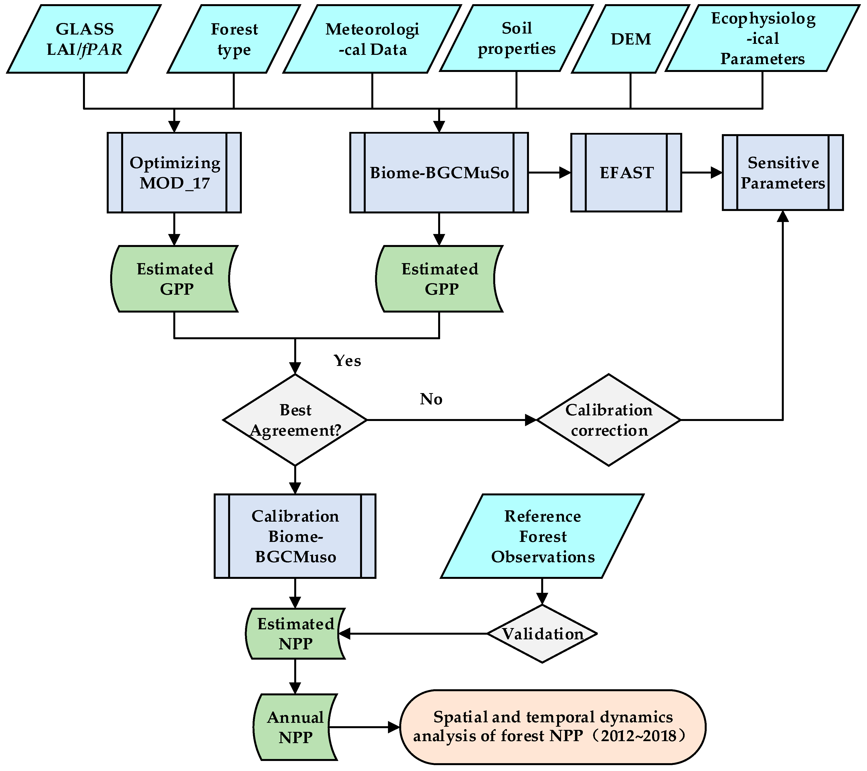
To assess the spatiotemporal dynamic changes in forest NPP, the method we used included four steps: first, the MOD_17 model was optimized using CMFD data, GLASS LAI/fPAR products, and the value of ε max for the main forest types in the study area; second, Biome-BGCMuSo was subjected to sensitivity analysis using the EFAST method, and the most sensitive parameters were retained for the next calibration step; third, sample plots representing different forest types were selected in the region, and the process model’s sensitive parameters for each forest type were calibrated based on the model–model coupling method; and fourth, the simulated forest NPP was validated using dendrochronological measurements, together with the spatiotemporal dynamic changes in forest NPP and its relationship with climatic factors were analyzed. Figure 2 shows the overall flowchart of the approach used in this study. Details of each step are given in subsequent sections.

2.3.1. The MOD_17 Model

The MOD_17 model [36] was developed according to the radiation conversion efficiency theory of Monteith [37], a remote sensing-based light energy utilization model. The MODIS GPP algorithm can be expressed as:
GPP   = ε max  ×  f ( T min )  ×  f ( VPD )  ×  APAR
APAR = PAR × f PAR
where ε max is the maximum LUE; PAR is the incident photosynthetically active radiation; f PAR is the fraction of PAR absorbed by vegetation; f ( T min ) and f ( VPD ) are the scalars of the minimum air temperature and VPD, respectively. The values of f ( T min ) and f ( VPD ) vary from in the range of [0, 1]. The expressions of f ( T min ) and f ( VPD )   are as follows:
f ( T min ) = {   0 , T min < T minmin T min - T minmin T minmax - T minmin , T minmin < T min < T minmax   1 , T min > T minmax
f ( VPD ) = {   0 , VPD > VPD max VPD max - VPD VPD max - VPD min , VPD min < VPD < VPD max 1 , VPD < VPD min
where VPD and T min are 8-day averaged values, and T minmin , T minmax , VPD max , and VPD min are parameters derived from Biome Properties Look-Up Table, and their values vary with vegetation types.
In this study, we first collected ε max for the test site according to the literature studied at similar study areas with similar latitudes consistent with the cold-temperate vegetation of the Greater Khingan Range (Table S1). Then, we used the processed meteorological data to optimize f ( T min ) and f ( VPD ) . Finally, the GLASS LAI/fPAR products were used to simulate the different forest-type GPP values from 2012 to 2015 and the values were used to calibrate the Biome-BGCMuSo model.

2.3.2. Biome-BGCMuSo Model

The Biome-BGCMuSo model was developed from the Biome-BGC model series [38], and we use the latest version of the model, Biome-BGCMuSo 6.2. Compared with Biome-BGC, Biome BGCMuSo improves the model’s ability to simulate carbon and water cycles in managed ecosystems and provides options for managing cropland, grassland, and forest, among which the most important modules of the model are the carbon flux module, phenology module and soil flux module. The GPP of vegetation is calculated by Farquhar’s [39] photosynthetic reaction mechanism model in the carbon flux module, and maintenance respiration is a function of reactive nitrogen content. Leaf development affects the accumulation of carbon and nitrogen in leaves, stems, roots, and litter, and is calculated by the phenology module. The soil flux module describes the decomposition of dead plant material and soil carbon pools [40].
The time scale of the Biome-BGCMuSo model is daily, and at least four input files are used for each execution: they are initialization file (INI file), meteorological data file (MET file), soil property file (SOIL file), and physiological ecological parameter file (EPC file). The simulation process of the model is divided into two stages: the first phase is the spinup simulation, where the model runs from a lower soil carbon and nitrogen level and it stops until a steady state is reached; the second phase is the normal simulation stage, which uses the initial values obtained in the initialization stage to simulate NPP of GPP [38]. To bring the model to an equilibrium state, daily meteorological data from 1992 to 2018 were selected and used in this study; in the procedure, the first 20 years were used for the spinup simulation phase and the last 7 years for the normal simulation phase.

2.3.3. Sensitivity Analysis

The EFAST method is a global sensitivity analysis method of model variance analysis proposed by Sailteli et al. [41], which combines the advantages of the Sobel method and the Fourier amplitude sensitivity test method. It has the advantages both of stability and fast calculation. Considering the complexity of the physiological and ecological parameters of the Biome-BGCMuSo model and the close interaction between the parameters, the influence of each physiological and ecological parameter on the output of the model is mainly represented by the first-order sensitivity index and the total sensitivity index. The first-order sensitivity index mainly reflects how much the variance of the model output can be reduced when a certain parameter value is fixed as the true value. The total sensitivity index refers to the sum of the first-order sensitivity index and the interaction sensitivity index between this parameter and other parameters. The total sensitivity index is suitable for global, quantitative, and model-independent sensitivity analysis.
The EFAST method often uses a search function to search in the multidimensional space of parameters, and obtains the sensitivity index by estimating the contribution rate of each data input Xi to the variance of the result Y, which can be expressed as:
Y = f ( X ) = f ( X 1 , X 2 , , X n )
where Xi (n = i) indicates that each input parameter has its own value range to indicate its uncertainty. The total variance of the model output can be expressed as:
V Y = i V i + i j > i k > j V ijk + + V 1 , 2 , . n  
where V i = V ( E ( Y / X i = x i * ) ) , V ij = V ( E ( Y X i = x i * , X i = x j * ) ) - V i - V j , and other variance calculation methods can be deduced in turn. E ( Y / X I = x i * ) represents the expected value of Y when Xi takes a fixed value xi. The first-order sensitivity index of the parameter S i = V i / V has a value range between 0 and 1, and the sensitivity index quantifies the influence of the parameter Xi on the results. The total sensitivity index STi is the sum of the first-order sensitivity index of this parameter and the interaction sensitivity index of this parameter with other parameters: S Ti = S i + S ij + S ijk + S ijk + S ijk m [42].
Sensitivity analysis of the Biome-BGCMuSo model was carried out in SimLab2.2. A total of 51 parameters were selected in the EPC input file (Table 1), and the variation range of each parameter was fluctuated around 20% [43]. To evaluate the selected 51 input parameters, we first sampled each parameter uniformly by the Monte Carlo method according to its range (Tables S2, S3 and S4), with a sampling frequency of 3315 (51 × 65) for each forest type. The total sampling frequency was 9945 (3315 × 3). Next, the Biome-BGCMuSo model was run in batches with the generated multiple sets of input parameters, and the statistical annual GPP averages of different forest types from 2012 to 2018 were input into SimLab2.2 for sensitivity analysis. Finally, the sensitivity indices (Si and STi) were divided into 3 groups: the indices with values greater than 0.2 were set as high sensitivity indices; the values between 0.1 and 0.2 were set as medium sensitivity indices; and the indices with values less than 0.1 were set as low sensitivity indices.

2.3.4. Incorporation of the MOD_17 and Biome-BGCMuSo

After sensitivity analysis by the EFAST method, the sensitive parameters of the Biome-BGCMuSo model (sensitivity index greater than 0.1) were retained, the sensitivity parameters were sorted according to the level of the parameter sensitivity, and the sensitivity parameters were calibrated for each forest type with respect to specific environmental factors. First, we selected sample points (30 for each type) of each forest type and its different ecological gradients (site conditions, meteorological conditions, stand structure, productivity, etc.) to simulate GPP from 2012 to 2015 (the number of samples is: 30 × 4 years × 23 layers × 3 = 8280). Then, the optimized MOD_17 model was used to fit the GPP simulation values of the Biome-BGCMuSo model corresponding to the spatiotemporal scale. During the fitting process, the parameters were adjusted according to the order of the sensitivity index. The globally representative calibration parameters in the process model are obtained when the fitting results are stable.

3. Results

3.1. Optimization of the MOD_17 Model

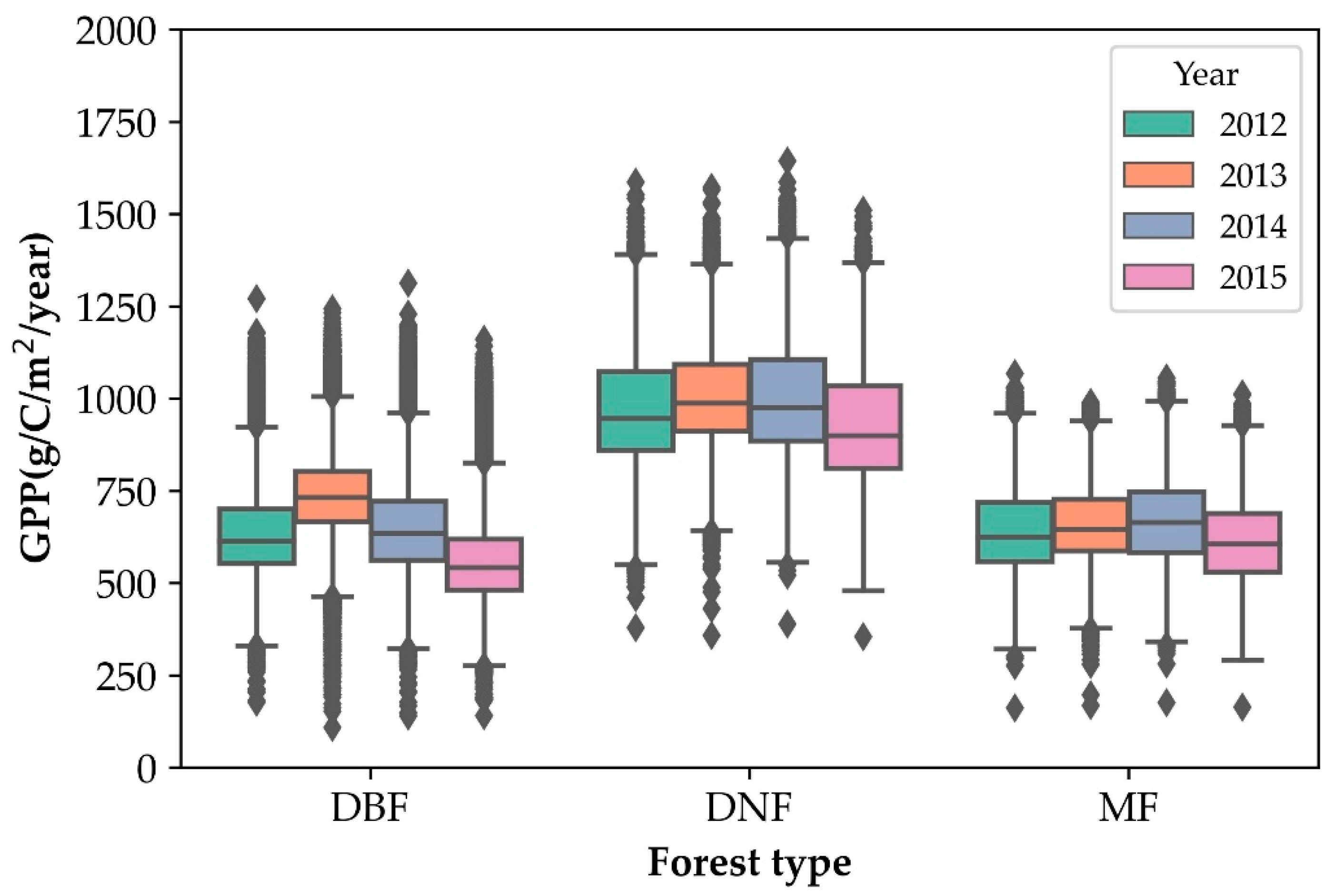
The optimized MOD_17 model was used to estimate the forest GPP in the Greater Khingan Mountains forest area of Inner Mongolia. Figure 3 shows the distribution of GPP in different forest types in 2012, 2013, 2014, and 2015. The highest GPP values was acquired by deciduous coniferous forest (DNF), next was deciduous broad-leaved forest (DBF), then the third was mixed coniferous (MF).
The highest value for DBF GPP was in 2013 and the highest value for DNF and MF GPP was in 2014. Table 2 shows the descriptive statistical results of the annual mean value of GPP for different forest types, including year, forest type, number of pixels (Count), mean (Mean), maximum value (Max), minimum value (Min), standard deviation (STD), and coefficient of variation (CV).
The uncertainty (CV) fluctuation of DBF had the largest range, spanning from 16.1% to 22.39%, and the range of GPP value was 108.4–1312.03 g/C/m2/year. The smallest uncertainty fluctuation range of DNF ranged from 14.34% to 17.03%, and the GPP value range was from 353.94 to 1643.15 g/C/m2/year. In general, the uncertainty fluctuation range of GPP was [14.34%, 22.39%], the annual average value of GPP ranged from 561.34 to 1008.21 g/C/m2/year, and the range of GPP value was [108.4, 1643.15] g/C/m2/year.

3.2. Sensitivity Analysis of Biome-BGCMuSo

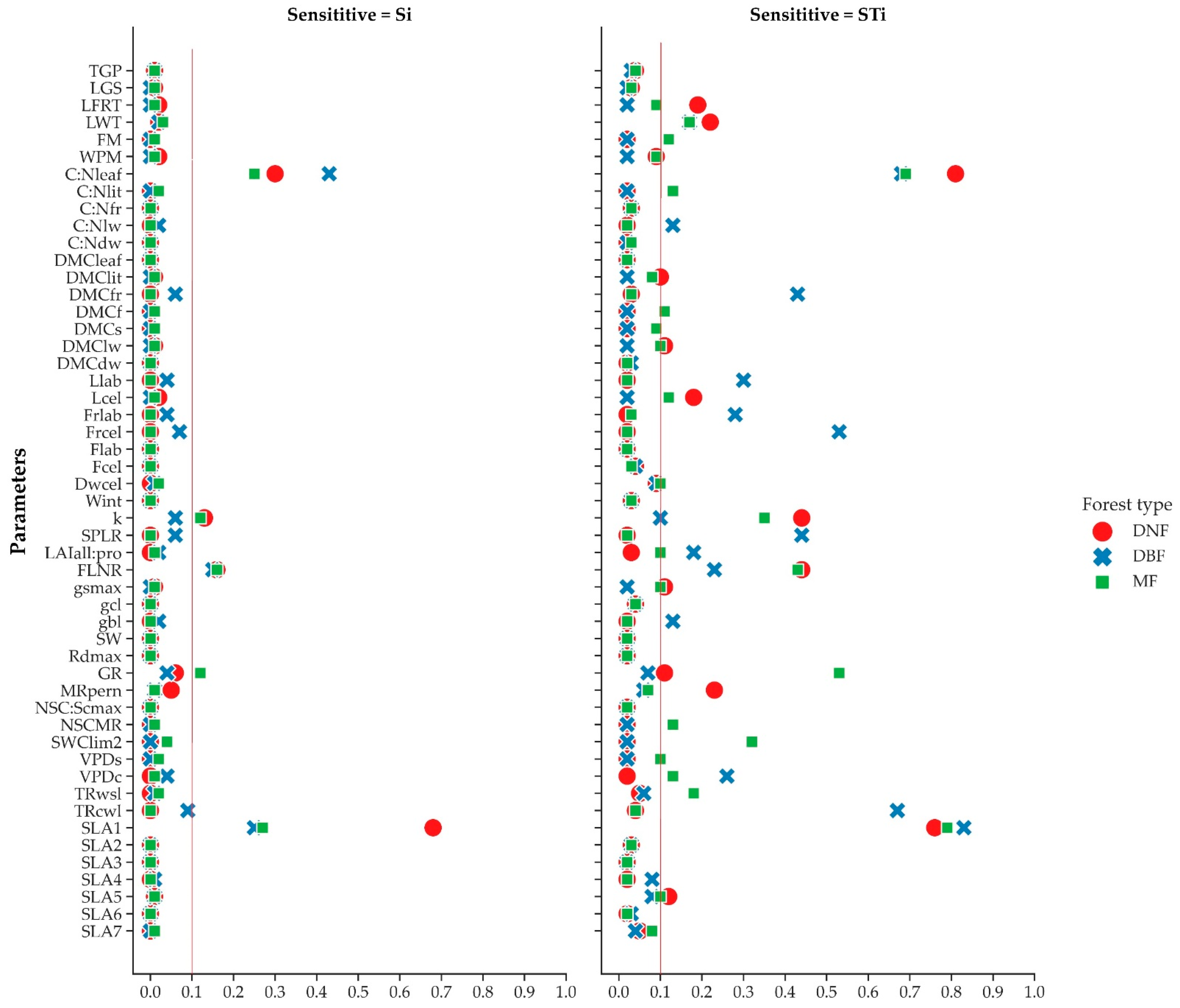
The mean annual GPP of different forest types in the study area and the first-order sensitivity index (Si) and total sensitivity index (STi) of the selected 51 parameters are shown in Figure 4, and the sensitive parameters are on the right side of the red solid line. The total sensitivity index was greater than the first-order sensitivity index, indicating that the interaction among the 51 parameters was much larger than the influence of a single parameter. The most sensitive first-order sensitivity and total sensitivity index of the annual GPP mean of DNF, DBF and MF were C:Nleaf and SLA1. The first-order sensitivity index was 0.3, 0.43 and 0.25, respectively, and the second-order sensitivity was 0.81, 0.68 and 0.69, respectively.
The mean annual GPPs of the different forest types are all sensitive to five parameters, namely C:Nleaf, SLA1, k, FLNR and LWT. It is worth noting that the sensitivity parameters were also different between the forest types, where MF and DBF were both sensitive to TRwsl and VPDc, while DNF was not sensitive to these two parameters.

3.3. Calibration of Biome-BGCMuSo Mode

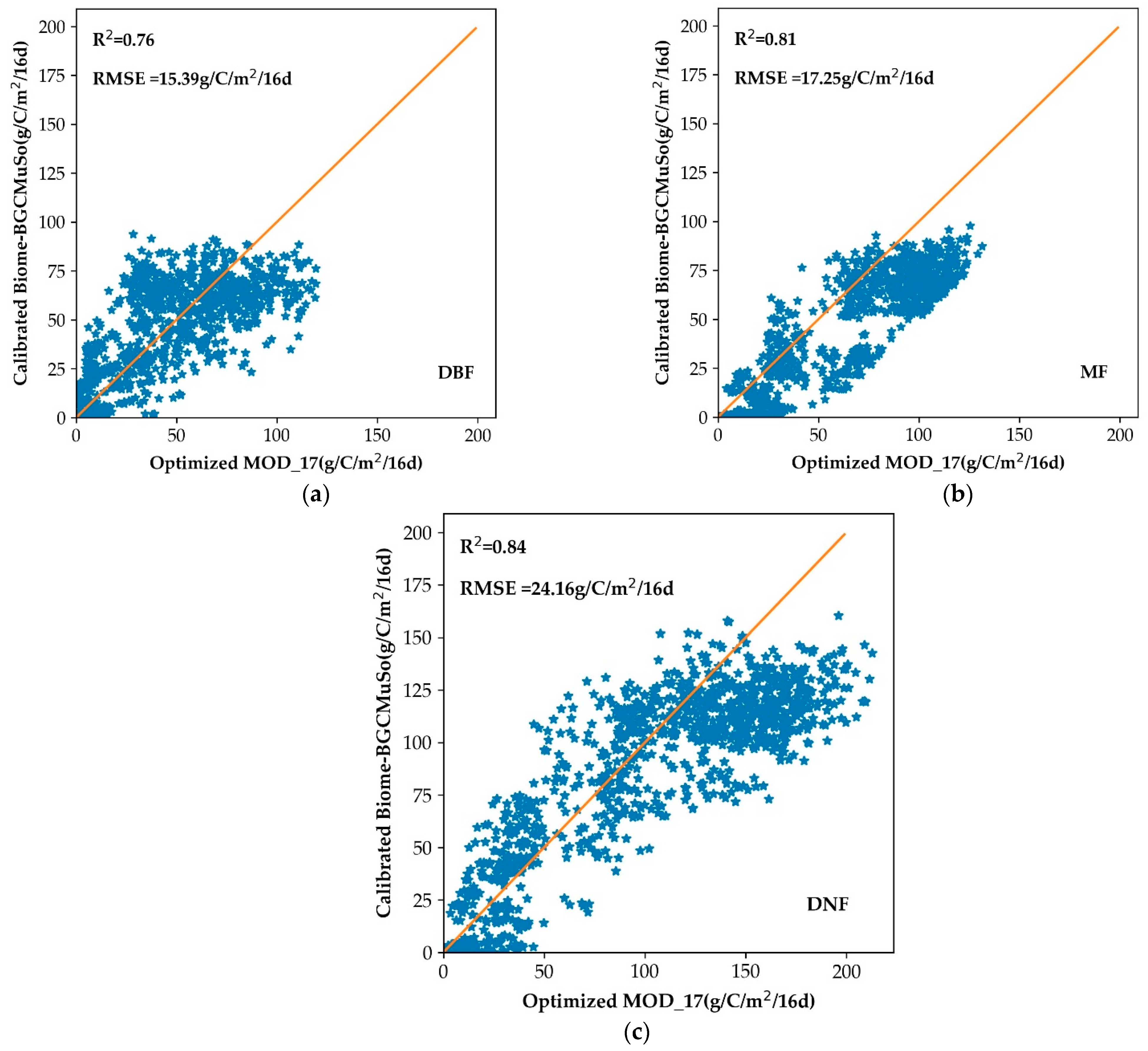
After the EFAST method was used to analyze the sensitivity of the physiological and ecological parameters of the Biome-BGCMuSo model, the results of calibrating the sensitive parameters of the model for different forest types were shown in Figure 5. The GPP values simulated by the optimized MOD_17 model are in agreement with the GPP values simulated by the calibrated Biome-BGCMuSo model. The best effect is DNF, R2 = 0.84, RMSE = 24.16 g/C/m2/16d; followed by MF, with R2 = 0.81 and RMSE = 17.25 g/C/m2/16d; the last one is DBF, with R2 = 0.76 and RMSE = 15.39 g/C/m2/16d.
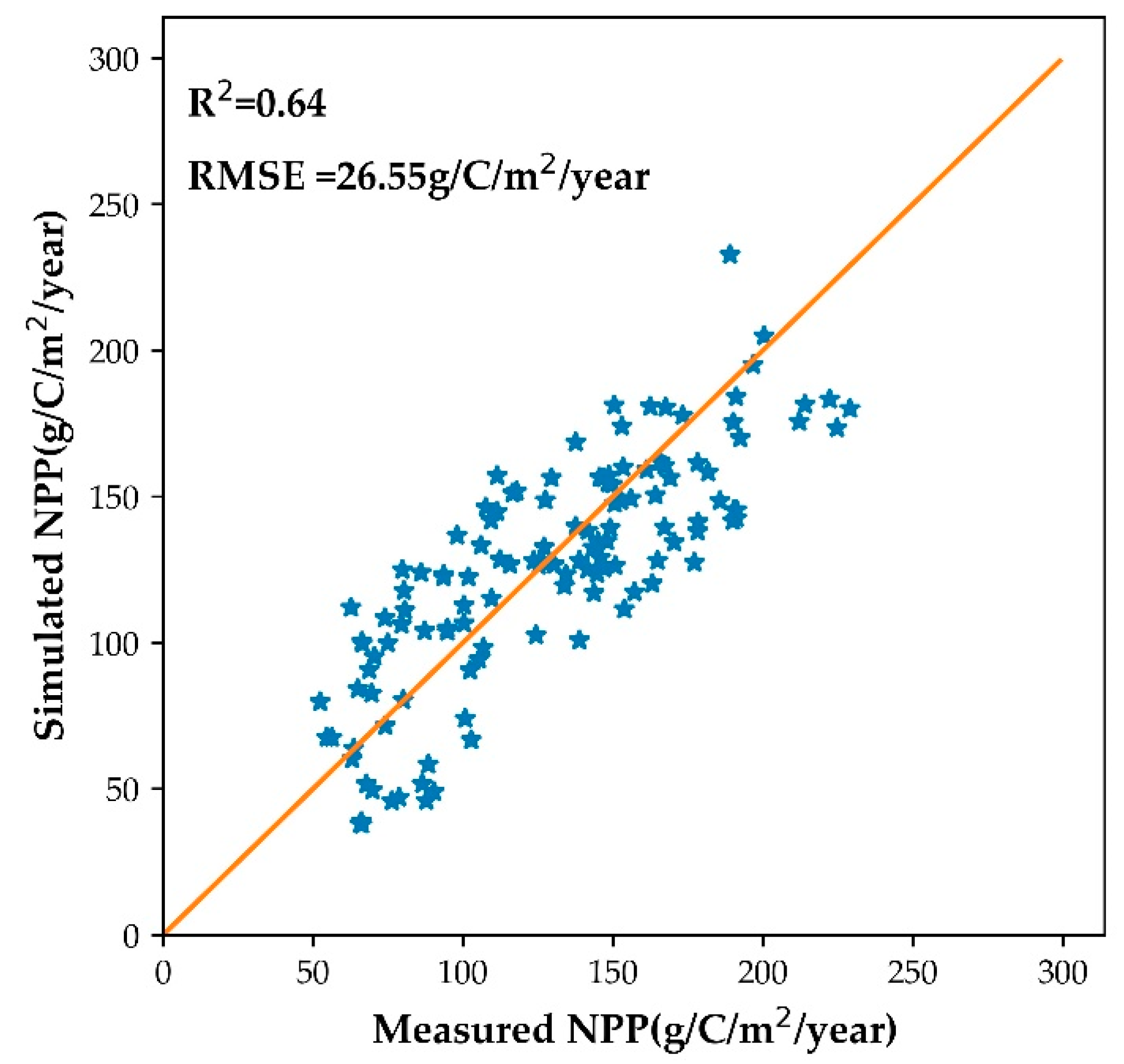
Through the dendrochronological measurements of 46 sample plots collected in the Greater Khingan Mountains area of Inner Mongolia in 2013 and 2016, some samples with serious interference and large measurement errors were screened. After conversion to forest NPP, they were verified with the calibrated Biome-BGCMuSo model. The results are as follows (Figure 6). The verification results showed that the calibrated Biome-BGCMuSo model simulates the forest NPP better, with R2 = 0.64 and RMSE = 26.55 g/C/m2/year.

3.4. The Spatial and Temporal Dynamics Analysis of Forest NPP

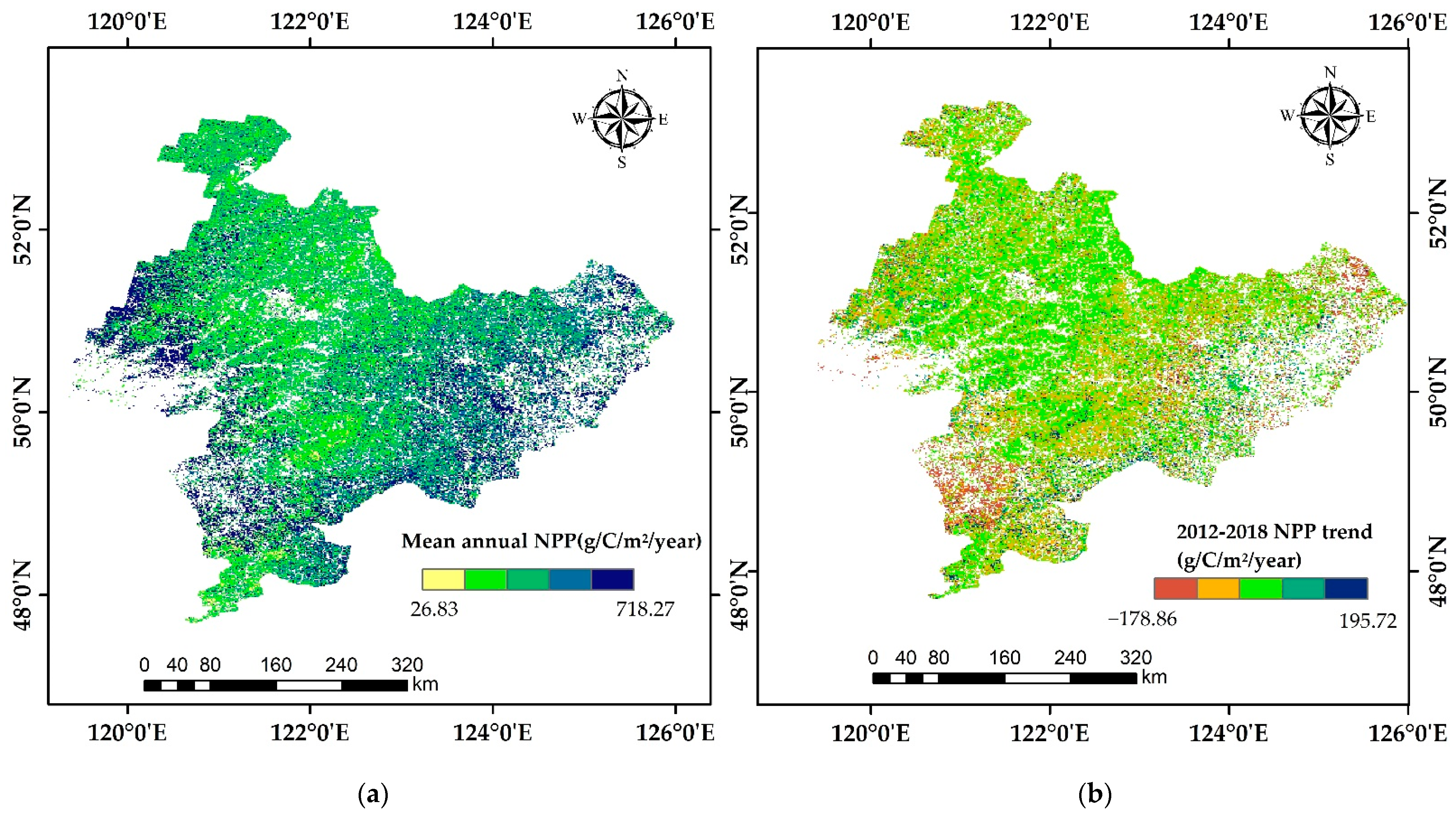
To analyze the temporal and spatial trends of forest NPP in the study area, the calibrated Biome-BGCMuSo simulated forest NPP in the study area and calculated the average forest NPP from 2012 to 2018. The results are shown in Figure 7a. The annual mean value of forest NPP ranged from 26.83 to 718.27 g/C/m2/year, which was low in the middle and high in the east and west in terms of spatial distribution. Figure 7b shows the forest NPP variation trend from 2012 to 2018. It revealed that the temporal variation trend of forest NPP was not obvious. The variation range of most areas was between −42.25 and 2.5 g/C/m2/year, while the regional change trend was obvious and showed a negative growth trend. Figure 8 shows the time distribution trend of NPP in different forest types in the growing season from 2012 to 2018. The highest NPP value in the growing season is coming from deciduous coniferous forest (DNF), next was coniferous and broad-leaved mixed forest (MF), the third was deciduous broad-leaved forest (DBF). During the seven-year period, the NPP in the growing season did not change significantly and showed a slow growth trend.
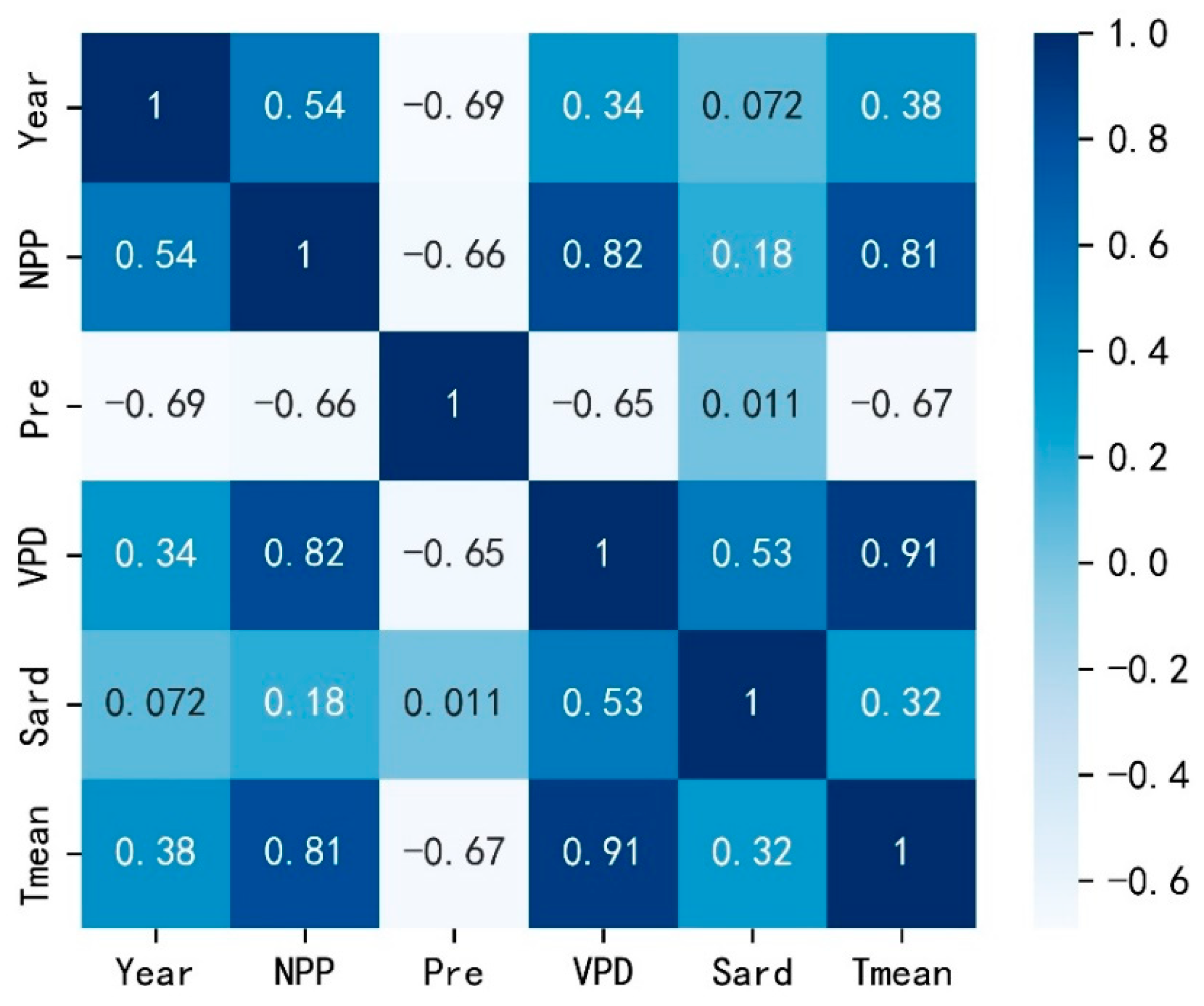
Figure 9 shows the correlation analysis results of the annual mean value of NPP and climatic factors in the forest growing season in the Greater Khingan Mountains forest area of Inner Mongolia. The correlation coefficient matrix (Figure 9) shows that the annual mean NPP of the forest growing season from 2012 to 2018 has an upward trend with a correlation coefficient of 0.54. The annual mean value of NPP in the forest growing season was positively and strongly correlated with VPD and Tmean, which were 0.82 and 0.81, respectively. The weak correlation with Sard was 0.11 and the negative correlation with PRE was −0.66.
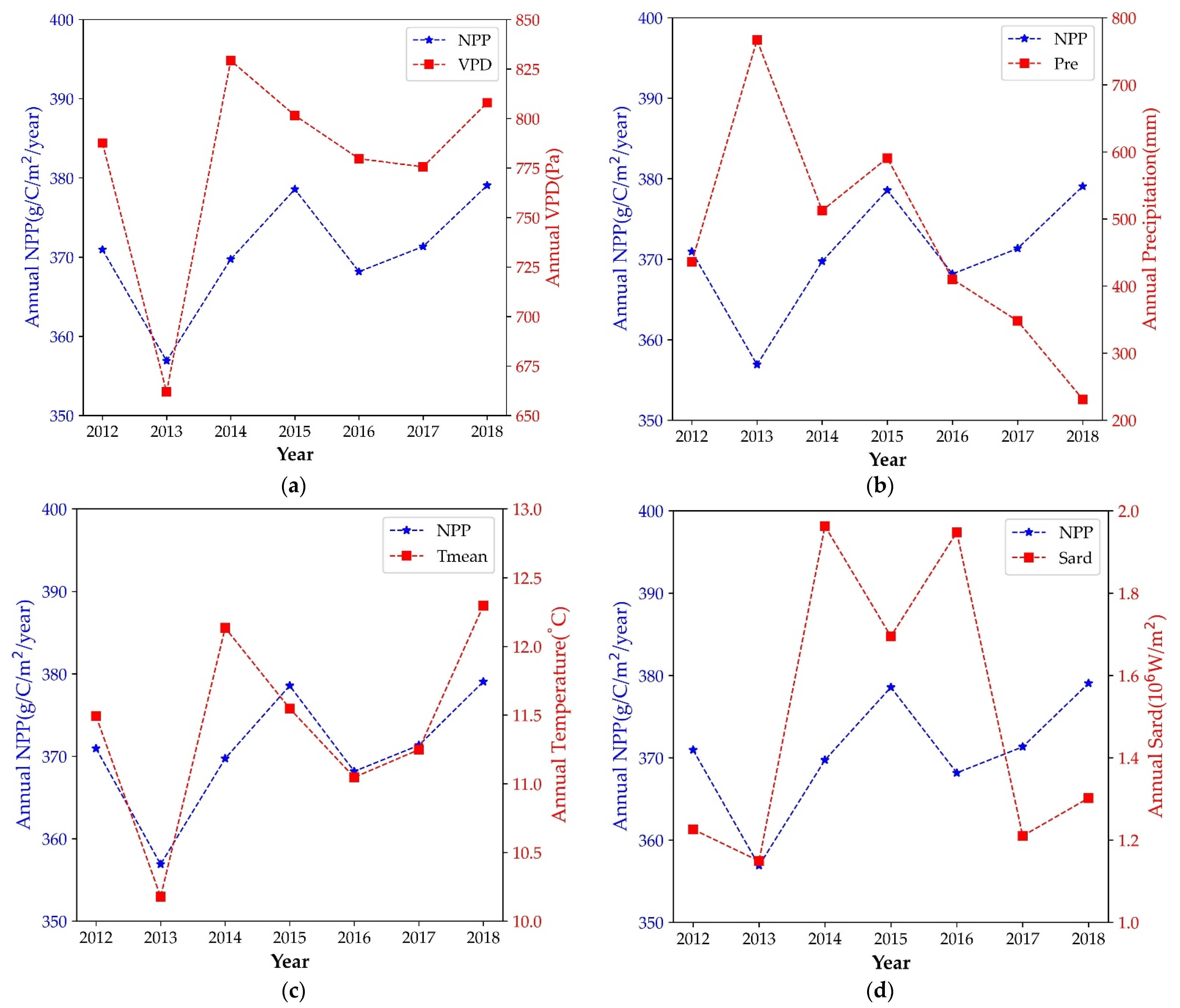
Figure 10 shows the statistical results of the annual average forest NPP dynamics and climatic factors in the Greater Khingan Mountains forest area of Inner Mongolia. The statistical data were only calculated for the forest growing season. From 2012 to 2018, the average temperature of the growing season in the study area was between 10.1~12.3 (°C), the annual precipitation was between 230~770 (mm), the average saturated vapor pressure was between 660~830 (Pa), and the annual shortwave radiation was 1.14~1.95 (106 W/m2). Among them, the change trend of forest NPP was basically consistent with the change trend of average vapor pressure and average temperature, which was opposite to the change trend of annual precipitation and the change trend of annual shortwave radiation was not obvious.

4. Discussion

This study showed that the incorporation strategy of the MOD_17 model and the Biome-BGCMuSo model can effectively reduce the uncertainty during the simulation of carbon fluxes in different forest types at the Greater Khingan Mountains, Inner Mongolia, in the cold temperate zone. By calibrating the MOD_17 model with the optimized Biome-BGCMuSo model, the correlation coefficient between the simulated forest NPP and the measured forest NPP was 0.64. Although the model was not validated with observational data such as flux sites in the study area, the simulation results were validated with two sample plot data points and tree dendrochronological measurements. Compared with the observation data such as flux sites, the sample plot data and dendrochronological measurement data had the characteristics of various disturbance scenarios and multihabitat conditions, strong spatial continuity, long-term scales, and many samples; the phenomenon revealed the effectiveness of the simulation through the incorporation model strategy and confirmed the reliability and global representation of forest carbon fluxes simulation.
The MOD_17 model has strong practicability and has been widely used at regional, national and even global scales, but the parameters of the Biome Properties Look-Up Table have significant uncertainties, which depend on the quality of remote sensing data, model parameterization schemes and empirical knowledge [44,45]. Therefore, we optimized each parameter. Among them, ε max had not been recalibrated but the ε max consistent with the cold temperate forest type had been collected through the literature data. The f ( T min ) , f ( VPD ) , and PAR were calculated from CMFD data with a time-resolve of 3 h [31], providing a basis for obtaining carbon fluxes with temporal and spatial continuity. The fPAR was derived from the GLASS LAI/fPAR product, which had been proven to be reliable [35].
Biome-BGCMuSo is a newly developed process model of Biome-BGC that is widely used to simulate forest NPP, but the sensitivity analysis of many parameters and model calibration are the key steps in forest carbon flux simulation. The results of our sensitivity analysis of the Biome-BGCMuSo model showed that there were five sensitive parameters that had important effects on different forest types. However, many parameters in the Biome-BGCMuSo model were extremely insensitive to GPP, such as TGP (transfer growth period as a fraction of growing season), LGS (litterfall as a fraction of growing season), DMCleaf (dry matter carbon content of leaves), DMCf (dry matter carbon content of fine roots), etc. The parameters that controlled the carboxylation rate of photosynthesis, such as C:Nleaf, SLA1 and FLNR, had the greatest impact on the GPP of different forest types, and the results were consistent with White et al. [43] and Ren et al. [46]. These three parameters determined the size of the maximum carboxylation rate, and the Rubisco enzyme directly affected the carboxylation of vegetation to fix atmospheric CO2. If the nitrogen content of Rubisco enzyme increased its activity would be promoted, thereby enhancing photosynthesis and promoting organic substance accumulation [47,48].
A strategy based on the incorporation of parametric models and ecological process models to simulate carbon fluxes with temporal and spatial continuity had been proven to be reliable and effective for Mediterranean forests and single dominant tree species in cold temperate zones [23,24,25,26], but feasibility experiments had not been carried out on different forest types in the cold temperate zone. Due to the heterogeneity of the growth environment, different forest types and the same forest type under different habitats had different physiological and ecological adaptation mechanisms, so it was difficult to calibrate the parameters of the Biome-BGCMuSo model on a regional basis, and it would result in the model distortion simulation [23]. Therefore, by incorporating the optimized MOD_17 model and the calibrated Biome-BGCMuSo model, it was effective to suppress the simulation of different forest types and it was possible to simulate carbon flux with spatial and temporal continuity.
Although we have reduced the uncertainty of the carbon flux simulation of different forest types in the Greater Khingan Mountains forest area of Inner Mongolia through the model–model coupling strategy, the simulation scale of the Biome-BGCMuSo model is 1 km, so the problem of pixel mixing cannot be avoided. The key to solving this problem is to use high-resolution remote sensing products. Although the classification products used in this study are fine classification products with a resolution of 30 m, the problem of pixel mixing cannot be avoided after resampling to 1 km. In addition, due to differences in model structure, parameter values, and driving data among different models, even if the coupling between models can improve the global representation of sensitivity parameter calibration, there are still errors in the simulation of forest ecological processes in large-area time series. In the model simulation, state parameters (such as LAI, soil moisture, freeze-thaw state, etc.) have large uncertainties, which will cause error transmission during the simulation process. Data assimilation is an objective and quantitative analysis method that integrates observations with heterogeneous, irregular distributions and different precisions on various types of spatiotemporal scales into the model, and obtains the best guesses for model parameters and state variables as much as possible [49].
The response of forest NPP to climate change is complex, and different forest types vary greatly. Climate controls the formation of forest NPP by changing environmental conditions to affect the physiological structure and process of forests, so changes in NPP can reflect the response of forest ecosystems to the environmental climate [50]. Generally, forest NPP has a positive response to precipitation changes, and has both positive and negative responses to temperature changes, but the response to temperature is stronger than that to precipitation. This study found that from 2012 to 2018, the forest NPP in the Greater Khingan Mountains, Inner Mongolia, had a positive response to the average temperature and average saturated vapor pressure, which was consistent with the results of He et al. [51] and Li et al. [52]. However, the difference is that we found a negative response between forest NPP and precipitation, which may have the following two reasons: First, the response of temperature to climate in the study area is much stronger than that of precipitation, especially in cold places. The annual average temperature in our selected study area is −3.5 °C and the extreme temperature reaches −50.2 °C, so the forest NPP may be more sensitive to temperature. Second, it may be due to the mutual interference of different climatic factors and the joint action of multiple factors. As shown in Figure 10, the minimum value of forest NPP in the study area was in 2013, and the average temperature, average saturated vapor pressure and annual shortwave radiation were the minimum values in 7 years, while the annual precipitation was the highest value in 7 years. Through the joint action of multiple factors, the stomatal conductance of plants is reduced or even closed, and both plant transpiration and photosynthesis are significantly reduced, thereby reducing the accumulation of dry matter.
From 2012 to 2018, the annual mean value of forest NPP ranged from 26.83 g to 718.27 g/C/m2/year, which was positively and strongly correlated with VPD and Tmean: 0.82 and 0.81, respectively. The weak correlation with Sard was 0.18, and the correlation with Pre was negatively correlated at −0.66. In terms of spatial distribution, it is low in the middle and high on the four sides; in terms of temporal trend, the change trend is not obvious, although it shows slow growth. The results showed that the GPP values of different forest types were highly sensitive to C:Nleaf (C:N of leaf), SLA1 (canopy average specific leaf area in phenological phase 1), and FLNR (fraction of leaf N in Rubisco).
In summary, this study also has some shortcomings, which can reduce the uncertainty sources of model simulation from the following aspects: (1) For the Biome-BGCMuSo model, site-specific input parameter values can achieve the best simulation of forest carbon flux, but some input parameters cannot be observed (such as Lcel, Llab, etc.), and it is difficult to obtain the variation range of parameters. How to collect and determine the range of these parameters needs to be further considered and explored; (2) The Biome BGCMuSo model improves the ability to simulate the carbon and water cycles in managed ecosystems. The simulation process is based on grids and does not consider the flow of matter and energy between grids; (3) We only used the sample plot data and dendrochronological measurement data to verify the results of forest carbon flux simulation in the study area, with low time resolution; (4) Although we simulated forest carbon flux with satisfactory spatial and temporal resolution through the strategy of model–model coupling, we did not consider disturbances such as forest diseases and insect pests, forest land changes, and forest fires.

5. Conclusions

Based on the strategy of incorporating the optimized remote sensing model and the ecological process model, this study simulated the carbon flux of different forest types in the Greater Khingan Mountains forest region of Inner Mongolia from 2012 to 2018, and then analyzed the spatial and temporal dynamic changes in forest carbon flux over the past 7 years. The results showed that C:Nleaf, SLA1 and FLNR were the most sensitive parameters of DNF, DBF and MF. Using the incorporation of optimized MOD_17 model and Biome-BGCMuSo, the simulated forest carbon flux can effectively suppress the distortion simulation of different forest types, which is verified by dendrochronological measurements data, and the effect is good.

Supplementary Materials

The following supporting information can be downloaded at: https://www.mdpi.com/article/10.3390/rs14194766/s1. Table S1. The values of maximum light use efficiency of various forest types; Table S2. Input parameters descriptions of DNF; Table S3. Input parameters descriptions of DBF; Table S4. Input parameters descriptions of MF.

Author Contributions

Conceptualization, X.T.; methodology, Y.S.; software, Y.S., B.L. and Y.M.; validation, Y.S., S.C. and H.W.; formal analysis, Y.S.; data curation, Y.S.; writing—original draft preparation, Y.S.; writing—review and editing, X.T., W.Z. and B.L.; visualization, Y.S.; supervision, W.Z.; project administration, X.T.; funding acquisition, X.T. and W. Z. All authors have read and agreed to the published version of the manuscript.

Funding

This research was funded by the National Natural Science Foundation of China (41871279, 32160365, 42161059 and 31860240), the Fundamental Research Funds of CAF (CAFYBB2021SY006), the National Science and Technology Major Project of China’s High Resolution Earth Observation System (21-Y20B01-9001-19/22).

Data Availability Statement

The data that support the findings of this study are available from the corresponding author, upon reasonable request.

Acknowledgments

Appreciation is extended to the Biome-BGCMuSo group for allowing free and open access to the model’s code. We would also like to thank Beijing Normal University for providing the GLASS products. The soil texture data set was sourced from Data Center for Resources and Environmental Sciences, Chinese Academy of Sciences (RESDC) (http://www.resdc.cn (accessed on 29 July 2021)).

Conflicts of Interest

The authors declare that they have no competing interests.

References

  1. Pan, Y.; Birdsey, R.A.; Fang, J.; Houghton, R.; Kauppi, P.E.; Kurz, W.A.; Phillips, O.L.; Shvidenko, A.; Lewis, S.L.; Canadell, J.G.; et al. A large and persistent carbon sink in the world’s forests. Science 2011, 333, 988–993. [Google Scholar] [CrossRef] [PubMed]
  2. Tang, S.; Wang, X.; He, M.; Huang, L.; Zhang, Y.; Yang, H.; Piao, S. Global Patterns and Climate Controls of Terrestrial Ecosystem Light Use Efficiency. J. Geophys. Res. Biogeosciences 2020, 125, e2020JG005908. [Google Scholar] [CrossRef]
  3. Zhao, J.; Liu, D.; Cao, Y.; Zhang, L.; Peng, H.; Wang, K.; Xie, H.; Wang, C. An integrated remote sensing and model approach for assessing forest carbon fluxes in China. Sci. Total Environ. 2022, 811, 152480. [Google Scholar] [CrossRef]
  4. Gray, A.N.; Whittier, T.R. Carbon stocks and changes on Pacific Northwest national forests and the role of disturbance, management, and growth. For. Ecol. Manag. 2014, 328, 167–178. [Google Scholar] [CrossRef]
  5. Sinha, S.K.; Padalia, H.; Patel, N.R.; Chauhan, P. Modelling sun-induced fluorescence for improved evaluation of forest carbon flux (GPP): Case study of tropical deciduous forest, India. Ecol. Model. 2021, 449, 109552. [Google Scholar] [CrossRef]
  6. Cook-Patton, S.C.; Leavitt, S.M.; Gibbs, D.; Harris, N.L.; Lister, K.; Anderson-Teixeira, K.J.; Briggs, R.D.; Chazdon, R.L.; Crowther, T.W.; Ellis, P.W.; et al. Mapping carbon accumulation potential from global natural forest regrowth. Nature 2020, 585, 545–550. [Google Scholar] [CrossRef] [PubMed]
  7. Zhou, T.; Shi, P.; Jia, G.; Luo, Y. Nonsteady state carbon sequestration in forest ecosystems of China estimated by data assimilation. J. Geophys. Res. Biogeosciences 2013, 118, 1369–1384. [Google Scholar] [CrossRef]
  8. Zhao, J.; Xie, H.; Ma, J.; Wang, K. Integrated remote sensing and model approach for impact assessment of future climate change on the carbon budget of global forest ecosystems. Glob. Planet. Chang. 2021, 203, 103542. [Google Scholar] [CrossRef]
  9. Kang, F.; Li, X.; Du, H.; Mao, F.; Zhou, G.; Xu, Y.; Huang, Z.; Ji, J.; Wang, J. Spatiotemporal Evolution of the Carbon Fluxes from Bamboo Forests and their Response to Climate Change Based on a BEPS Model in China. Remote Sens. 2022, 14, 366. [Google Scholar] [CrossRef]
  10. Zhang, H.; Tang, S.; Wang, F. Study on establish and estimate method of biomass model compatible with volume. For. Res. 1999, 12, 53–59. [Google Scholar] [CrossRef]
  11. Ciais, P.; Reichstein, M.; Viovy, N.; Granier, A.; Ogée, J.; Allard, V.; Aubinet, M.; Buchmann, N.; Bernhofer, C.; Carrara, A. Europe-wide reduction in primary productivity caused by the heat and drought in 2003. Nature 2005, 437, 529–533. [Google Scholar] [CrossRef] [PubMed]
  12. Kljun, N.; Black, T.A.; Griffis, T.J.; Barr, A.G.; Gaumont-Guay, D.; Morgenstern, K.; McCaughey, J.H.; Nesic, Z. Response of net ecosystem productivity of three boreal forest stands to drought. Ecosystems 2007, 10, 1039–1055. [Google Scholar] [CrossRef]
  13. Chirici, G.; Chiesi, M.; Corona, P.; Salvati, R.; Papale, D.; Fibbi, L.; Sirca, C.; Spano, D.; Duce, P.; Marras, S.; et al. Estimating daily forest carbon fluxes using a combination of ground and remotely sensed data. J. Geophys. Res. Biogeosciences 2016, 121, 266–279. [Google Scholar] [CrossRef]
  14. Wen, J.; You, D.; Han, Y.; Lin, X.; Wu, S.; Tang, Y.; Xiao, Q.; Liu, Q. Estimating Surface BRDF/Albedo Over Rugged Terrain Using an Extended Multisensor Combined BRDF Inversion (EMCBI) Model. IEEE Geosci. Remote Sens. Lett. 2022, 19, 1–5. [Google Scholar] [CrossRef]
  15. Potter, C.S.; Randerson, J.T.; Field, C.B.; Matson, P.A.; Vitousek, P.M.; Mooney, H.A.; Klooster, S.A. Terrestrial ecosystem production: A process model based on global satellite and surface data. Glob. Biogeochem. Cycles 1993, 7, 811–841. [Google Scholar] [CrossRef]
  16. Prince, S.D.; Goward, S.N. Global Primary Production: A Remote Sensing Approach. J. Biogeogr. 1995, 22, 815–835. [Google Scholar] [CrossRef]
  17. Running, S.W.; Nemani, R.; Glassy, J.M.; Thornton, P.E. MODIS Daily Photosynthesis (PSN) and Annual Net Primary Production (NPP) Product (MOD17) Algorithm Theoretical Basis Document. University of Montana, SCFAt-Launch Algorithm ATBD Documents. Available online: www.ntsg.umt.edu/files/modis/ATBD_MOD17_v21.pdf (accessed on 16 October 2021).
  18. Veroustraete, F.; Sabbe, H.; Eerens, H. Estimation of carbon mass fluxes over Europe using the C-Fix model and Euroflux data. Remote Sens. Environ. 2002, 83, 376–399. [Google Scholar] [CrossRef]
  19. Running, S.W.; Hunt, E.R. Generalization of a Forest Ecosystem Process Model for Other Biomes, BIOME-BGC, and an Application for Global-Scale Models. In Scaling Physiological Processes; Ehleringer, J.R., Field, C.B., Eds.; Academic Press: San Diego, CA, USA, 1993; pp. 141–158. [Google Scholar] [CrossRef]
  20. Melillo, J.M.; McGuire, A.D.; Kicklighter, D.W.; Moore, B.; Vorosmarty, C.J.; Schloss, A.L. Global climate change and terrestrial net primary production. Nature 1993, 363, 234–240. [Google Scholar] [CrossRef]
  21. Liu, J.; Chen, J.M.; Park, W.M. A process-based boreal ecosystem productivity simulator using remote sensing inputs. Remote Sens. Environ. 1997, 62, 158–175. [Google Scholar] [CrossRef]
  22. Thornton, P.E.; Law, B.E.; Gholz, H.L.; Clark, K.L.; Falge, E.; Ellsworth, D.S.; Goldstein, A.H.; Monson, R.K.; Hollinger, D.; Falk, M. Modeling and measuring the effects of disturbance history and climate on carbon and water budgets in evergreen needleleaf forests. Agric. For. Meteorol. 2002, 113, 185–222. [Google Scholar] [CrossRef]
  23. Chiesi, M.; Maselli, F.; Moriondo, M.; Fibbi, L.; Bindi, M.; Running, S.W. Application of Biome-BGC to simulate Mediterranean forest processes. Ecol. Model. 2007, 206, 179–190. [Google Scholar] [CrossRef]
  24. Yan, M.; Tian, X.; Li, Z.; Chen, E.; Wang, X.; Han, Z.; Sun, H. Simulation of Forest Carbon Fluxes Using Model Incorporation and Data Assimilation. Remote Sens. 2016, 8, 567. [Google Scholar] [CrossRef]
  25. Tian, X.; Yan, M.; van der Tol, C.; Li, Z.; Su, Z.; Chen, E.; Li, X.; Li, L.; Wang, X.; Pan, X.; et al. Modeling forest above-ground biomass dynamics using multi-source data and incorporated models: A case study over the qilian mountains. Agric. For. Meteorol. 2017, 246, 1–14. [Google Scholar] [CrossRef]
  26. Yan, M.; Tian, X.; Li, Z.; Chen, E.; Li, C.; Fan, W. A long-term simulation of forest carbon fluxes over the Qilian Mountains. Int. J. Appl. Earth Obs. Geoinf. 2016, 52, 515–526. [Google Scholar] [CrossRef]
  27. Sánchez-Ruiz, S.; Maselli, F.; Chiesi, M.; Fibbi, L.; Martínez, B.; Campos-Taberner, M.; García-Haro, F.J.; Gilabert, M.A. Remote Sensing and Bio-Geochemical Modeling of Forest Carbon Storage in Spain. Remote Sens. 2020, 12, 1356. [Google Scholar] [CrossRef]
  28. Zhang, X.; Zhang, Q.; Sun, S.; Xu, Z.; Jian, Y.; Yang, Y.; Tian, Y.; Sa, R.; Wang, B.; Wang, F. Carbon exchange characteristics and their environmental effects in the northern forest ecosystem of the Greater Khingan Mountains in China. Sci. Total Environ. 2022, 838, 156056. [Google Scholar] [CrossRef]
  29. Yang, K.; He, J. China Meteorological Forcing Dataset (1979–2018); National Tibetan Plateau Data Center, Ed.; National Tibetan Plateau Data Center: Beijing, China, 2019. [Google Scholar] [CrossRef]
  30. He, J.; Yang, K.; Tang, W.; Lu, H.; Qin, J.; Chen, Y.; Li, X. The first high-resolution meteorological forcing dataset for land process studies over China. Sci. Data 2020, 7, 25. [Google Scholar] [CrossRef]
  31. Yang, K.; He, J.; Tang, W.; Qin, J.; Cheng, C.C.K. On downward shortwave and longwave radiations over high altitude regions: Observation and modeling in the Tibetan Plateau. Agric. For. Meteorol. 2010, 150, 38–46. [Google Scholar] [CrossRef]
  32. Dong, L.; Li, F.; Jia, W.; Liu, F.; Wang, H. Compatible biomass models for main tree species with measurement error in Heilongjiang Province of Northeast China. Chin. J. Appl. Ecol. 2011, 22, 2653–2661. [Google Scholar] [CrossRef]
  33. Wu, G.; Feng, Z. Study on the biomass of larix spp. forest community in the frigid-temperate zone and the temperate zone of China. J. Northeast For. Univ. 1995, 23, 95–101. [Google Scholar] [CrossRef]
  34. Li, H.; Lei, Y. Estimation and Evaluation of Forest Biomass Carbon Storage in China; China Forestry Publishing House: Beijing, China, 2010. [Google Scholar]
  35. Xiao, Z.; Liang, S.; Wang, J.; Chen, P.; Yin, X.; Zhang, L.; Song, J. Use of general regression neural networks for generating the GLASS leaf area index product from time-series MODIS surface reflectance. IEEE Trans. Geosci. Remote Sens. 2014, 52, 209–223. [Google Scholar] [CrossRef]
  36. Running, S.W.; Thornton, P.E.; Nemani, R.; Glassy, J.M. Global terrestrial gross and net primary productivity from the earth observing system. In Methods in Ecosystem Science; Sala, O.E., Jackson, R.B., Mooney, H.A., Howarth, R.W., Eds.; Springer: New York, NY, USA, 2000. [Google Scholar] [CrossRef]
  37. Monteith, J.L. Solar radiation and productivity in tropical ecosystems. J. Appl. Ecol. 1972, 9, 747–766. [Google Scholar] [CrossRef]
  38. Hidy, D.; Barcza, Z.; Hollós, R.; Thornton, P.E.; Running, S.W.; Fodor, N. User’s Guide for Biome-BGCMuSo 6.2. Available online: https://nimbus.elte.hu/bbgc/files/Manual_BBGC_MuSo_v6.2.pdf (accessed on 17 November 2021).
  39. Farquhar, G.D.; von Caemmerer, S.; Berry, J.A. A biochemical model of photosynthetic CO2 assimilation in leaves of C 3 species. Planta 1980, 149, 78–90. [Google Scholar] [CrossRef] [PubMed]
  40. Hidy, D.; Barcza, Z.; Marjanović, H.; Ostrogović Sever, M.Z.; Dobor, L.; Gelybó, G.; Fodor, N.; Pintér, K.; Churkina, G.; Running, S.; et al. Terrestrial ecosystem process model Biome-BGCMuSo v4.0: Summary of improvements and new modeling possibilities. Geosci. Model Dev. 2016, 9, 4405–4437. [Google Scholar] [CrossRef]
  41. Saltelli, A.; Tarantola, S.; Chan, K.P.S. A Quantitative Model-Independent Method for Global Sensitivity Analysis of Model Output. Technometrics 1999, 41, 39–56. [Google Scholar] [CrossRef]
  42. Campolongo, F.; Saltelli, A.; Tarantola, S. Sensitivity Anaysis as an Ingredient of Modeling. Stat. Sci. 2000, 15, 377–395. [Google Scholar] [CrossRef]
  43. White, M.A.; Thornton, P.E.; Running, S.W.; Nemani, R.R. Parameterization and sensitivity analysis of the Biome–BGC terrestrial ecosystem model: Net primary production controls. Earth Interact. 2000, 4, 1–85. [Google Scholar] [CrossRef]
  44. Huang, X.; Xiao, J.; Wang, X.; Ma, M. Improving the global MODIS GPP model by optimizing parameters with FLUXNET data. Agric. For. Meteorol. 2021, 300, 108314. [Google Scholar] [CrossRef]
  45. Li, X.; Liang, H.; Cheng, W. Evaluation and comparison of light use efficiency models for their sensitivity to the diffuse PAR fraction and aerosol loading in China. Int. J. Appl. Earth Obs. Geoinf. 2021, 95, 102269. [Google Scholar] [CrossRef]
  46. Ren, H.; Zhang, L.; Yan, M.; Tian, X.; Zheng, X. Sensitivity analysis of Biome-BGCMuSo for gross and net primary productivity of typical forests in China. For. Ecosyst. 2022, 9, 100011. [Google Scholar] [CrossRef]
  47. Houborg, R.; Cescatti, A.; Migliavacca, M. Constraining model simulations of GPP using satellite retrieved leaf chlorophyll. In Proceedings of the Geoscience and Remote Sensing Symposium (IGARSS), 2012 IEEE International, Munich, Germany, 22–27 July 2012. [Google Scholar]
  48. Li, X.H.; Sun, J.X. Testing parameter sensitivities and uncertainty analysis of Biome-BGC model in simulating carbon and water fluxes in broadleaved-korean pine forests. Chin. J. Plant Ecol. 2018, 42, 1131–1144. [Google Scholar] [CrossRef]
  49. Li, X.; Ma, H.; Ran, Y.; Wang, X.; Zhu, G.; Liu, F.; He, H.; Zhang, Z.; Huang, C. Terrestrial carbon cycle model-data fusion: Progress and challenges. Sci. Sin. Terrae 2021, 64, 1650–1663. [Google Scholar] [CrossRef]
  50. Xu, Y.; Xiao, F.; Yu, L. Review of spatio-temporal distribution of net primary productivity in forest ecosystem and its responses to climate change in China. Acta Ecol. Sin. 2020, 40, 4710–4723. [Google Scholar] [CrossRef]
  51. He, L.; Wan, H.; Wang, L.; Wang, Y. Response of net primary productivity of Larix olgensis forest ecosystem to climate change. J. Beijing For. Univ. 2015, 37, 28–36. [Google Scholar] [CrossRef]
  52. Li, Y.; Wang, Y.; Sun, Y.J.; Lei, Y.C.; Shao, W.C.; Li, J. Temporal-spatial characteristics of NPP and its response to climate change of Larix forests in Jilin Province. Acta Ecol. Sin. 2022, 42, 947–959. [Google Scholar] [CrossRef]
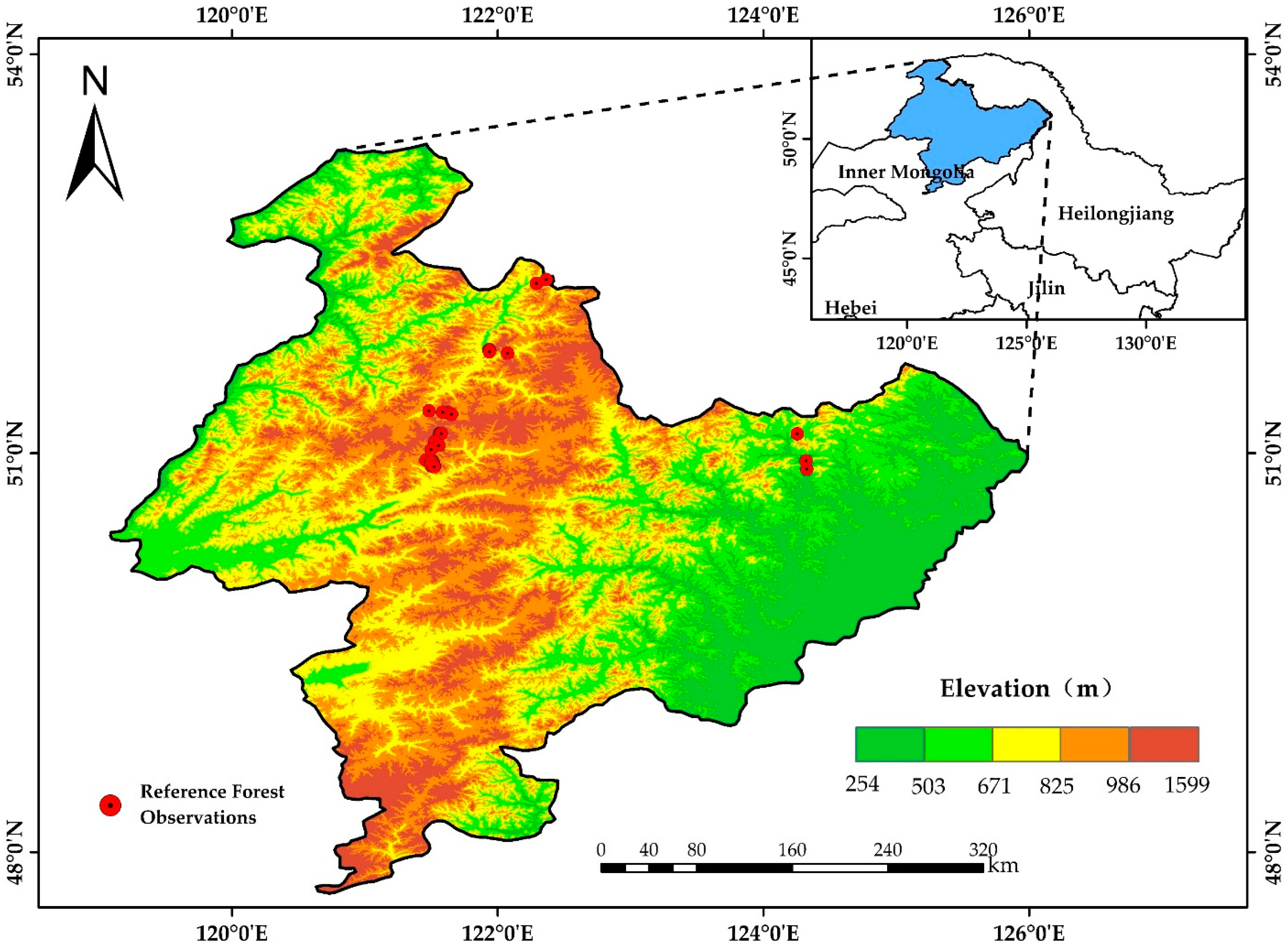
Figure 1. The location and forest observation sample sites in the Greater Khingan Mountains in Inner Mongolia.
Remotesensing 14 04766 g001
Figure 2. Overall flow chart of this study.
Remotesensing 14 04766 g002
Figure 3. The distribution of GPP in the Greater Khingan Mountains in Inner Mongolia from 2012 to 2015.
Remotesensing 14 04766 g003
Figure 4. First-order Sensitivity Index (Si) and Total Sensitivity Index (STi) for GPPs of different forest types.
Remotesensing 14 04766 g004
Figure 5. Comparison of 16-day GPP values fitted by the optimized MOD_17 model and the calibrated Biome-BGCMuSo model.
Remotesensing 14 04766 g005
Figure 6. Validation of interannual NPP of the calibrated Biome-BGCMuSo model with NPP from dendrochronological data time series.
Remotesensing 14 04766 g006
Figure 7. The spatial distribution of average annual NPP (a), and its changing trend (b) from 2012 to 2018.
Remotesensing 14 04766 g007
Figure 8. The distribution of different forest types in growing season NPP from 2012 to 2018.
Remotesensing 14 04766 g008
Figure 9. Correlation coefficient (r) matrix of NPP and meteorological data in growing seasons in the Greater Khingan Mountains in Inner Mongolia.
Remotesensing 14 04766 g009
Figure 10. Interannual NPP and meteorological data statistics for the growing seasons in forested areas over the Greater Khingan Mountains in Inner Mongolia.
Remotesensing 14 04766 g010
Table 1. Selected input parameters of Biome-BGCMuSo used in the sensitivity analysis.
NumberParameterDescriptionUnit
1TGPtransfer growth period as fraction of growing seasonprop.
2LGSlitterfall as fraction of growing seasonprop.
3LFRTannual leaf and fine root turnover fraction 1/yr
4LWTannual live wood turnover fraction1/yr
5FMannual fire mortality fraction1/yr
6WPMwhole-plant mortality fraction in vegetation period1/yr
7C:NleafC:N of leaveskgC/kg N
8C:NlitC:N of leaf litter, after retranslocation kgC/kg N
9C:NfrC:N of fine rootskgC/kg N
10C:NlwC:N of live woodkgC/kg N
11C:NdwC:N of dead woodkgC/kg N
12DMCleafdry matter carbon content of leaves(kgC/kgDM)
13DMClitdry matter carbon content of leaf litter(kgC/kgDM)
14DMCfrdry matter carbon content of fine roots(kgC/kgDM)
15DMCfdry matter carbon content of fruit(kgC/kgDM)
16DMCsdry matter carbon content of soft stem(kgC/kgDM)
17DMClwdry matter carbon content of live wood(kgC/kgDM)
18DMCdwdry matter carbon content of dead wood(kgC/kgDM)
19Llableaf litter labile proportionDIM
20Lcelleaf litter cellulose proportionDIM
21FRlabP fine root labile proportionDIM
22FRcelfine root cellulose proportionDIM
23Flabfruit litter labile proportionDIM
24Fcelfruit litter cellulose proportionDIM
25DWceldead wood cellulose proportionDIM
26Wintcanopy water interception coefficient 1/LAI/d
27kcanopy light extinction coefficientDIM
28SPLRall-sided to projected leaf area ratioDIM
29LAIall:proratio of shaded SLA:sunlit SLADIM
30FLNRfraction of leaf N in RubiscoDIM
31gsmaxmaximum stomatal conductance (projected area basis)m/s
32gclconductance (projected area basis)m/s
33gblboundary layer conductance (projected area basis)m/s
34SWstem weight corresponding to maximum height(kgC)
35Rdmaxmaximum depth of rooting zone(m)
36GRgrowth resp per unit of C grown(prop.)
37MRpernmaintenance respiration in kg C/day per kg of tissue N(kgC/kgN/d)
38NSC:Scmaxtheoretical maximum prop. of non-structural and structural carbohydrates(DIM)
39NSCMRof non-structural carbohydrates available for maintenance respiration(DIM)
40SWClim2minimum of soil moisture limit2 multiplicator (full anoxic stress value)prop
41VPDsvapor pressure deficit: start of conductance reductionPa
42VPDcvapor pressure deficit: complete conductance reductionPa
43TRwslturnover rate of wilted standing biomass to litterprop
44TRcwlturnover rate of non-woody cut-down biomass to litterprop
45SLA1canopy average specific leaf area in phenological phase 1m2/kg
46SLA2canopy average specific leaf area in phenological phase 2m2/kg
47SLA3canopy average specific leaf area in phenological phase 3m2/kg
48SLA4canopy average specific leaf area in phenological phase 4m2/kg
49SLA5canopy average specific leaf area in phenological phase 5m2/kg
50SLA6canopy average specific leaf area in phenological phase 6m2/kg
51SLA7canopy average specific leaf area in phenological phase 7m2/kg
Table 2. GPP statistical results of the MOD_17 model simulation after optimization.
YearForest TypeCountMeanSTDMinMaxCV (%)
2012DBF41,583635.48130.39176.431269.9520.52
DNF7651977.62160.46378.921585.8216.41
MF22,631641.17114.07160.941067.5217.79
2013DBF41,580737.82118.83108.41242.416.1
DNF76511008.21144.6357.081571.6914.34
MF22,630657.27102.53167.75989.1615.6
2014DBF41,575646.63139.75138.711312.0321.61
DNF76501000.89158.98388.921643.1515.88
MF22,628665.82114.89175.51055.1617.25
2015DBF41,578561.34125.7139.761160.0822.39
DNF7649927.53157.95353.941509.9317.03
MF22,628611.4110.91163.671012.618.14
Publisher’s Note: MDPI stays neutral with regard to jurisdictional claims in published maps and institutional affiliations.